Estimating the Number of Connected Components in a Graph via Subgraph Sampling

Abstract

Learning properties of large graphs from samples has been an important problem in statistical network analysis since the early work of Goodman [27] and Frank [21]. We revisit a problem formulated by Frank [21] of estimating the number of connected components in a large graph based on the subgraph sampling model, in which we randomly sample a subset of the vertices and observe the induced subgraph. The key question is whether accurate estimation is achievable in the sublinear regime where only a vanishing fraction of the vertices are sampled. We show that it is impossible if the parent graph is allowed to contain high-degree vertices or long induced cycles. For the class of chordal graphs, where induced cycles of length four or above are forbidden, we characterize the optimal sample complexity within constant factors and construct linear-time estimators that provably achieve these bounds. This significantly expands the scope of previous results which have focused on unbiased estimators and special classes of graphs such as forests or cliques.

Both the construction and the analysis of the proposed methodology rely on combinatorial properties of chordal graphs and identities of induced subgraph counts. They, in turn, also play a key role in proving minimax lower bounds based on construction of random instances of graphs with matching structures of small subgraphs.

1 Introduction

Counting the number of features in a graph – ranging from basic local structures like motifs or graphlets (e.g., edges, triangles, wedges, stars, cycles, cliques) to more global features like the number of connected components – is an important task in network analysis. For example, the global clustering coefficient of a graph (i.e. the fraction of closed triangles) is a measure of the tendency for nodes to cluster together and a key quantity used to study cohesion in various networks [42]. To learn these graph properties, applied researchers typically collect data from a random sample of nodes to construct a representation of the true network. We refer to these problems collectively as statistical inference on sampled networks, where the goal is to infer properties of the parent network (population) from a subsampled version. Below we mention a few examples that arise in various fields of study.

• Sociology: Social networks of the Hadza hunter-gatherers of Tanzania were studied in [3] by surveying 205 individuals in 17 Hadza camps (from a population of 517). Another study [12] of farmers in Ghana used network data from a survey of 180 households in three villages from a population of 550 households.

• Economics and business: Low sampling ratios have been used in applied economics (such as 30% in [18]), particularly for large scale studies [4, 19]. A good overview of various experiments in applied economics and their corresponding sampling ratios can be found in [9, Appendix F, p. 11]. Word of mouth marketing in consumer referral networks was studied in [49] using 158 respondents from a potential subject pool of 238.

• Genomics: The authors of [53] use protein-protein interaction data and demonstrate that it is possible to arrive at a reliable statistical estimate for the number of interactions (edges) from a sample containing approximately 1500 vertices.

• World Wide Web and Internet: Informed random IP address probing was used in [29] in an attempt to obtain a router-level map of the Internet.

As mentioned earlier, a primary concern of these studies is how well the data represent the true network and how to reconstruct the relevant properties of the parent graphs from samples. These issues and how they are addressed broadly arise from two perspectives:

• The full network is unknown due to the lack of data, which could arise from the underlying experimental design and data collection procedure, e.g., historical or observational data. In this case, one needs to construct statistical estimators (i.e., functions of the sampled graph) to conduct sound inference. These estimators must be designed to account for the fact that the sampled network is only a partial observation of the true network, and thus subject to certain inherent biases and variability.

• The full network is either too large to scan or too expensive to store. In this case, approximation algorithms can overcome such computational or storage issues that would otherwise be unwieldy. For example, for massive social networks, it is generally impossible to enumerate the whole population. Rather than reading the entire graph, query-based algorithms randomly (or deterministically) sample parts of the graph or adaptively explore the graph through a random walk [5]. Some popular instances of traversal based procedures are snowball sampling [28] and respondent-driven sampling [52]. Indeed, sampling (based on edge and degree queries) is a commonly used primitive to speed up computation, which leads to various sublinear-time algorithms for testing or estimating graph properties such as the average degree [25], triangle and more general subgraph counts [15, 2], expansion properties [26]; we refer the readers to the monograph [23].

Learning properties of graphs from samples has been an important problem in statistical network analysis since the early work of Goodman [27] and Frank [21]. Estimation of various properties such as graph totals [20] and connectivity [8, 21] has been studied in a variety of sample models. However, most of the analysis has been confined to obtaining unbiased estimators for certain classes of graphs and little is known about their optimality. The purpose of this paper is to initiate a systematic study of statistical inference on sampled networks, with the goal of determining their statistical limits in terms of minimax risks and sample complexity, achieved by computationally efficient procedures.

As a first step towards this goal, in this paper we focus on a representative problem introduced in [21], namely, estimating the number of connected components in a graph from a partial sample of the population network. In fact, the techniques developed in this paper are also useful for estimating other graph statistics such as motif counts, which were studied in the companion paper [35].

Before we proceed, let us emphasize that the objective of this paper is not testing whether the graph is connected, which is a property too fragile to test on the basis of a small sampled graph; indeed, missing a single edge can destroy the connectivity. Instead, our goal is to estimate the number of connected components with an optimal additive accuracy. Thus, naturally, it is applicable to graphs with a large number of components.

We study the problem of estimating the number of connected components for two reasons. First, it encapsulates many challenging aspects of statistical inference on sampled graphs, and we believe the mathematical framework and machinery developed in this paper will prove useful for estimating other graph properties as well. Second, the number of connected components is a useful graph property that quantifies the connectivity of a network. In addition, it finds use in data-analytic applications related to determining the number of classes in a population [27]. Another example is the recent work [11], which studies the estimation of the number of documented deaths in the Syrian Civil War from a subgraph induced by a set of vertices obtained from an adaptive sampling process (similar to subgraph sampling). There, the goal is to estimate the number of unique individuals in a population, which roughly corresponds to the number of connected components in a network of duplicate records connected by shared attributes.

Next we discuss the sampling model, which determines how reflective the data is of the population graph and therefore the quality of the estimation procedure. There are many ways to sample from a graph (see [13, 39] for a list of techniques and [38, 37, 30] for comprehensive reviews). For simplicity, this paper focuses on the simplest sampling model, namely, subgraph sampling, where we randomly sample a subset of the vertices and observe their induced subgraph; in other words, only the edges between the sampled vertices are revealed. Results on estimating motif counts for the related neighborhood sampling model can be found in the companion paper [35]. One of the earliest works that adopts the subgraph sampling model is by Frank [21], which is the basis for the theory developed in this paper. Drawing from previous work on estimating population total using vertex sampling [20], Frank obtained unbiased estimators of the number of connected components and performance guarantees (variance calculations) for graphs whose connected components are either all trees or all cliques. Extensions to more general graphs are briefly discussed, although no unbiased estimators are proposed. This generality is desirable since it is more realistic to assume that the objects in each class (component) are in between being weakly and strongly connected to each other, corresponding to having the level of connectivity between a tree and clique. While the results of Frank are interesting, questions of their generality and optimality remain open and we therefore address these matters in the sequel. Specifically, the main goals of this paper are as follows:

• Characterize the sample complexity, i.e., the minimal sample size to achieve a given accuracy, as a function of graph parameters.

• Devise computationally efficient estimators that provably achieve the optimal sample complexity bound.

Of particular interest is the sublinear regime, where only a vanishing fraction of the vertices are sampled. In this case, it is impossible to reconstruct the entire graph, but it might still be possible to accurately estimate the desired graph property.

The problem of estimating the number of connected components in a large graph has also been studied in the computer science literature, where the goal is to design randomized algorithms with sublinear (in the size of the graph) time complexity. The celebrated work [10] proposed a randomized algorithm to estimate the number of connected components in a general graph (motivated by computing the weight of the minimum spanning tree) within an additive error of $\epsilon N$ for graphs with $N$ vertices and average degree $d_{\text{avg}}$, with runtime $O(\frac{d_{\text{avg}}}{\epsilon^{2}}\log\frac{d_{\text{avg}}}{\epsilon})$. Their method relies on data obtained from a random sample of vertices and then performing a breadth first search on each vertex which ends according to a random stopping criterion. The algorithm requires knowledge of the average degree $d_{\text{avg}}$ and must therefore be known or estimated a priori. The runtime was further improved to $O(\epsilon^{-2}\log\frac{1}{\epsilon})$ by modifying the stopping criterion [6]. In these algorithms, the breadth first search may visit many of the edges and explore a larger fraction of the graph at each round. From an applied perspective, such traversal based procedures can be impractical or impossible to implement in many statistical applications due to limitations inherent in the experimental design and it is more realistic to treat the network data as a random sample from a parent graph.

Finally, let us compare, conceptually, the framework in the present paper with the work on model-based network analysis, where networks are modeled as random graphs drawn from specific generative models, such as the stochastic block model [31], graphons [22], or exponential random graph models [32] (cf. the recent survey [38]), and performance analysis of statistical procedures for parameter estimation or clustering are carried out for these models. In contrast, in network sampling we adopt a design-based framework [30], where the graph is assumed to be deterministic and the randomness comes from the sampling process.

Organization

The paper is organized as follows. In Section 2, we formally define the estimation problem, the subgraph sampling model, and describe what classes of graphs we will be focusing on. To motivate our attention on specific classes of graphs (chordal graphs with maximum degree constraints), we show that in the absence of such structural assumptions, sublinear sample complexity is impossible in the sense that at least a constant faction of the vertices need to be sampled. Section 3 introduces the definition of chordal graphs and states our main results in terms of the minimax risk and sample complexity. In Section 4, after introducing the relevant combinatorial properties of chordal graphs, we define the estimator of the number of connect components and provide its statistical guarantees. We also propose a heuristic for constructing an estimator on non-chordal graphs. In Section 5, we develop a general strategy for proving minimax lower bound for estimating graph properties and particularize it to obtain matching lower bounds for the estimator constructed in Section 4.

Some of the technical proofs, additional results for the uniform sampling model and for forests and graphs with long cycles, and a numerical study of the proposed estimators on simulated data for various graphs are deferred till Appendix A, Appendix B, and Appendix C, respectively.

Notations

We use standard big-$O$ notations, e.g., for any positive sequences $\{a_{n}\}$ and $\{b_{n}\}$, $a_{n}=O(b_{n})$ or $a_{n}\lesssim b_{n}$ if $a_{n}\leq Cb_{n}$ for some absolute constant $C>0$, $a_{n}=o(b_{n})$ or $a_{n}\ll b_{n}$ or if $\lim a_{n}/b_{n}=0$. Furthermore, the subscript in $a_{n}=O_{r}(b_{n})$ means $a_{n}\leq C_{r}b_{n}$ for some constant $C_{r}$ depending on the parameter $r$ only. For positive integer $k$, let $[k]=\{1,\dots,k\}$. Let $\mathrm{Bern}(p)$ denote the Bernoulli distribution with mean $p$ and $\mathrm{Bin}(N,p)$ the binomial distribution with $N$ trials and success probability $p$.

Next we introduce some graph-theoretic notations that will be used throughout the paper. Let $G=(V,E)$ be a simple undirected graph. Let ${\mathsf{e}}={\mathsf{e}}(G)=|E(G)|$ denote the number of edges, ${\mathsf{v}}={\mathsf{v}}(G)=|V(G)|$ denote the number of vertices, and $\mathsf{cc}=\mathsf{cc}(G)$ be the number of connected components in $G$. The neighborhood of a vertex $u$ is denoted by $N_{G}(u)=\{v\in V(G):\{u,v\}\in E(G)\}$.

Two graphs $G$ and $G^{\prime}$ are isomorphic, denoted by $G\simeq G^{\prime}$, if there exists a bijection between the vertex sets of $G$ and $G^{\prime}$ that preserves adjacency, i.e., if there exists a bijective function $g:V(G)\to V(G^{\prime})$ such that $\{g(u),g(v)\}\in E(G^{\prime})$ if and only if $\{u,v\}\in E(G)$. The disjoint union of two graphs $G$ and $G^{\prime}$, denoted $G+G^{\prime}$, is the graph whose vertex (resp. edge) set is the disjoint union of the vertex (resp. edge) sets of $G$ and of $G^{\prime}$. For brevity, we denote by $kG$ to the disjoint union of $k$ copies of $G$.

We use the notation $K_{n}$, $P_{n}$, and $C_{n}$ to denote the complete graph, path graph, and cycle graph on $n$ vertices, respectively. Let $K_{n,n^{\prime}}$ denote the complete bipartite graph with $nn^{\prime}$ edges and $n+n^{\prime}$ vertices. Let $S_{n}$ denote the star graph $K_{1,n}$ on $n+1$ vertices.

We need two types of subgraph counts: Denote by $\mathsf{s}(H,G)$ (resp. $\mathsf{n}(H,G)$) the number of vertex (resp. edge) induced subgraphs of $G$ that are isomorphic to $H$. For example, $\mathsf{s}(\leavevmode\hbox to17.63pt{\vbox to3.4pt{\pgfpicture\makeatletter\hbox{\hskip 1.7pt\lower-1.7pt\hbox to0.0pt{\pgfsys@beginscope\pgfsys@invoke{ }\definecolor{pgfstrokecolor}{rgb}{0,0,0}\pgfsys@color@rgb@stroke{0}{0}{0}\pgfsys@invoke{ }\pgfsys@color@rgb@fill{0}{0}{0}\pgfsys@invoke{ }\pgfsys@setlinewidth{0.4pt}\pgfsys@invoke{ }\nullfont\pgfsys@beginscope\pgfsys@invoke{ }\pgfsys@invoke{\lxSVG@closescope }\pgfsys@endscope\hbox to0.0pt{\pgfsys@beginscope\pgfsys@invoke{ }{{}}{{}{{}}{}{{}} {}{}{{}} {}{}{{}}{}\pgfsys@moveto{0.0pt}{0.0pt}\pgfsys@lineto{7.11319pt}{0.0pt}\pgfsys@lineto{14.22638pt}{0.0pt}\pgfsys@stroke\pgfsys@invoke{ }\hbox{\hbox{\hbox{\hbox{{\pgfsys@beginscope\pgfsys@invoke{ }\definecolor[named]{pgffillcolor}{rgb}{1,1,1}\pgfsys@color@gray@fill{1}\pgfsys@invoke{ }{{}{{{}}}{{}}{}{}{}{}{}{}{}{}{}{\pgfsys@beginscope\pgfsys@invoke{ }\definecolor[named]{pgffillcolor}{rgb}{1,1,1}\pgfsys@color@gray@fill{1}\pgfsys@invoke{ }{}\pgfsys@moveto{1.5pt}{0.0pt}\pgfsys@curveto{1.5pt}{0.82843pt}{0.82843pt}{1.5pt}{0.0pt}{1.5pt}\pgfsys@curveto{-0.82843pt}{1.5pt}{-1.5pt}{0.82843pt}{-1.5pt}{0.0pt}\pgfsys@curveto{-1.5pt}{-0.82843pt}{-0.82843pt}{-1.5pt}{0.0pt}{-1.5pt}\pgfsys@curveto{0.82843pt}{-1.5pt}{1.5pt}{-0.82843pt}{1.5pt}{0.0pt}\pgfsys@closepath\pgfsys@moveto{0.0pt}{0.0pt}\pgfsys@fillstroke\pgfsys@invoke{ } \pgfsys@invoke{\lxSVG@closescope }\pgfsys@endscope}{{{{}}\pgfsys@beginscope\pgfsys@invoke{ }\pgfsys@transformcm{1.0}{0.0}{0.0}{1.0}{0.0pt}{0.0pt}\pgfsys@invoke{ }\hbox{{\definecolor{pgfstrokecolor}{rgb}{0,0,0}\pgfsys@color@rgb@stroke{0}{0}{0}\pgfsys@invoke{ }\pgfsys@color@rgb@fill{0}{0}{0}\pgfsys@invoke{ }\hbox{} }}\pgfsys@invoke{\lxSVG@closescope }\pgfsys@endscope}}} \pgfsys@invoke{\lxSVG@closescope }\pgfsys@endscope}}}\hbox{{\pgfsys@beginscope\pgfsys@invoke{ }\definecolor[named]{pgffillcolor}{rgb}{1,1,1}\pgfsys@color@gray@fill{1}\pgfsys@invoke{ }{{}{{{}}}{{}}{}{}{}{}{}{}{}{}{}{\pgfsys@beginscope\pgfsys@invoke{ }\definecolor[named]{pgffillcolor}{rgb}{1,1,1}\pgfsys@color@gray@fill{1}\pgfsys@invoke{ }{}\pgfsys@moveto{8.61319pt}{0.0pt}\pgfsys@curveto{8.61319pt}{0.82843pt}{7.94162pt}{1.5pt}{7.11319pt}{1.5pt}\pgfsys@curveto{6.28476pt}{1.5pt}{5.61319pt}{0.82843pt}{5.61319pt}{0.0pt}\pgfsys@curveto{5.61319pt}{-0.82843pt}{6.28476pt}{-1.5pt}{7.11319pt}{-1.5pt}\pgfsys@curveto{7.94162pt}{-1.5pt}{8.61319pt}{-0.82843pt}{8.61319pt}{0.0pt}\pgfsys@closepath\pgfsys@moveto{7.11319pt}{0.0pt}\pgfsys@fillstroke\pgfsys@invoke{ } \pgfsys@invoke{\lxSVG@closescope }\pgfsys@endscope}{{{{}}\pgfsys@beginscope\pgfsys@invoke{ }\pgfsys@transformcm{1.0}{0.0}{0.0}{1.0}{7.11319pt}{0.0pt}\pgfsys@invoke{ }\hbox{{\definecolor{pgfstrokecolor}{rgb}{0,0,0}\pgfsys@color@rgb@stroke{0}{0}{0}\pgfsys@invoke{ }\pgfsys@color@rgb@fill{0}{0}{0}\pgfsys@invoke{ }\hbox{} }}\pgfsys@invoke{\lxSVG@closescope }\pgfsys@endscope}}} \pgfsys@invoke{\lxSVG@closescope }\pgfsys@endscope}}}\hbox{{\pgfsys@beginscope\pgfsys@invoke{ }\definecolor[named]{pgffillcolor}{rgb}{1,1,1}\pgfsys@color@gray@fill{1}\pgfsys@invoke{ }{{}{{{}}}{{}}{}{}{}{}{}{}{}{}{}{\pgfsys@beginscope\pgfsys@invoke{ }\definecolor[named]{pgffillcolor}{rgb}{1,1,1}\pgfsys@color@gray@fill{1}\pgfsys@invoke{ }{}\pgfsys@moveto{15.72638pt}{0.0pt}\pgfsys@curveto{15.72638pt}{0.82843pt}{15.05481pt}{1.5pt}{14.22638pt}{1.5pt}\pgfsys@curveto{13.39795pt}{1.5pt}{12.72638pt}{0.82843pt}{12.72638pt}{0.0pt}\pgfsys@curveto{12.72638pt}{-0.82843pt}{13.39795pt}{-1.5pt}{14.22638pt}{-1.5pt}\pgfsys@curveto{15.05481pt}{-1.5pt}{15.72638pt}{-0.82843pt}{15.72638pt}{0.0pt}\pgfsys@closepath\pgfsys@moveto{14.22638pt}{0.0pt}\pgfsys@fillstroke\pgfsys@invoke{ } \pgfsys@invoke{\lxSVG@closescope }\pgfsys@endscope}{{{{}}\pgfsys@beginscope\pgfsys@invoke{ }\pgfsys@transformcm{1.0}{0.0}{0.0}{1.0}{14.22638pt}{0.0pt}\pgfsys@invoke{ }\hbox{{\definecolor{pgfstrokecolor}{rgb}{0,0,0}\pgfsys@color@rgb@stroke{0}{0}{0}\pgfsys@invoke{ }\pgfsys@color@rgb@fill{0}{0}{0}\pgfsys@invoke{ }\hbox{} }}\pgfsys@invoke{\lxSVG@closescope }\pgfsys@endscope}}} \pgfsys@invoke{\lxSVG@closescope }\pgfsys@endscope}}} } \pgfsys@invoke{\lxSVG@closescope }\pgfsys@endscope{}{}{}\hss}\pgfsys@discardpath\pgfsys@invoke{\lxSVG@closescope }\pgfsys@endscope\hss}}\lxSVG@closescope\endpgfpicture}},\;\leavevmode\hbox to10.51pt{\vbox to10.51pt{\pgfpicture\makeatletter\hbox{\hskip 1.7pt\lower-1.7pt\hbox to0.0pt{\pgfsys@beginscope\pgfsys@invoke{ }\definecolor{pgfstrokecolor}{rgb}{0,0,0}\pgfsys@color@rgb@stroke{0}{0}{0}\pgfsys@invoke{ }\pgfsys@color@rgb@fill{0}{0}{0}\pgfsys@invoke{ }\pgfsys@setlinewidth{0.4pt}\pgfsys@invoke{ }\nullfont\pgfsys@beginscope\pgfsys@invoke{ }\pgfsys@invoke{\lxSVG@closescope }\pgfsys@endscope\hbox to0.0pt{\pgfsys@beginscope\pgfsys@invoke{ }{{}}{{}{{}}{} {}{}{}\pgfsys@moveto{7.11319pt}{0.0pt}\pgfsys@lineto{0.0pt}{7.11319pt}\pgfsys@stroke\pgfsys@invoke{ } {}{{}}{}{{}} {}{}{{}} {}{}{{}} {}{}{{}} {}{}\pgfsys@moveto{0.0pt}{0.0pt}\pgfsys@lineto{7.11319pt}{0.0pt}\pgfsys@lineto{7.11319pt}{7.11319pt}\pgfsys@lineto{0.0pt}{7.11319pt}\pgfsys@closepath\pgfsys@stroke\pgfsys@invoke{ }\hbox{\hbox{\hbox{\hbox{\hbox{{\pgfsys@beginscope\pgfsys@invoke{ }\definecolor[named]{pgffillcolor}{rgb}{1,1,1}\pgfsys@color@gray@fill{1}\pgfsys@invoke{ }{{}{{{}}}{{}}{}{}{}{}{}{}{}{}{}{\pgfsys@beginscope\pgfsys@invoke{ }\definecolor[named]{pgffillcolor}{rgb}{1,1,1}\pgfsys@color@gray@fill{1}\pgfsys@invoke{ }{}\pgfsys@moveto{1.5pt}{0.0pt}\pgfsys@curveto{1.5pt}{0.82843pt}{0.82843pt}{1.5pt}{0.0pt}{1.5pt}\pgfsys@curveto{-0.82843pt}{1.5pt}{-1.5pt}{0.82843pt}{-1.5pt}{0.0pt}\pgfsys@curveto{-1.5pt}{-0.82843pt}{-0.82843pt}{-1.5pt}{0.0pt}{-1.5pt}\pgfsys@curveto{0.82843pt}{-1.5pt}{1.5pt}{-0.82843pt}{1.5pt}{0.0pt}\pgfsys@closepath\pgfsys@moveto{0.0pt}{0.0pt}\pgfsys@fillstroke\pgfsys@invoke{ } \pgfsys@invoke{\lxSVG@closescope }\pgfsys@endscope}{{{{}}\pgfsys@beginscope\pgfsys@invoke{ }\pgfsys@transformcm{1.0}{0.0}{0.0}{1.0}{0.0pt}{0.0pt}\pgfsys@invoke{ }\hbox{{\definecolor{pgfstrokecolor}{rgb}{0,0,0}\pgfsys@color@rgb@stroke{0}{0}{0}\pgfsys@invoke{ }\pgfsys@color@rgb@fill{0}{0}{0}\pgfsys@invoke{ }\hbox{} }}\pgfsys@invoke{\lxSVG@closescope }\pgfsys@endscope}}} \pgfsys@invoke{\lxSVG@closescope }\pgfsys@endscope}}}\hbox{{\pgfsys@beginscope\pgfsys@invoke{ }\definecolor[named]{pgffillcolor}{rgb}{1,1,1}\pgfsys@color@gray@fill{1}\pgfsys@invoke{ }{{}{{{}}}{{}}{}{}{}{}{}{}{}{}{}{\pgfsys@beginscope\pgfsys@invoke{ }\definecolor[named]{pgffillcolor}{rgb}{1,1,1}\pgfsys@color@gray@fill{1}\pgfsys@invoke{ }{}\pgfsys@moveto{8.61319pt}{0.0pt}\pgfsys@curveto{8.61319pt}{0.82843pt}{7.94162pt}{1.5pt}{7.11319pt}{1.5pt}\pgfsys@curveto{6.28476pt}{1.5pt}{5.61319pt}{0.82843pt}{5.61319pt}{0.0pt}\pgfsys@curveto{5.61319pt}{-0.82843pt}{6.28476pt}{-1.5pt}{7.11319pt}{-1.5pt}\pgfsys@curveto{7.94162pt}{-1.5pt}{8.61319pt}{-0.82843pt}{8.61319pt}{0.0pt}\pgfsys@closepath\pgfsys@moveto{7.11319pt}{0.0pt}\pgfsys@fillstroke\pgfsys@invoke{ } \pgfsys@invoke{\lxSVG@closescope }\pgfsys@endscope}{{{{}}\pgfsys@beginscope\pgfsys@invoke{ }\pgfsys@transformcm{1.0}{0.0}{0.0}{1.0}{7.11319pt}{0.0pt}\pgfsys@invoke{ }\hbox{{\definecolor{pgfstrokecolor}{rgb}{0,0,0}\pgfsys@color@rgb@stroke{0}{0}{0}\pgfsys@invoke{ }\pgfsys@color@rgb@fill{0}{0}{0}\pgfsys@invoke{ }\hbox{} }}\pgfsys@invoke{\lxSVG@closescope }\pgfsys@endscope}}} \pgfsys@invoke{\lxSVG@closescope }\pgfsys@endscope}}}\hbox{{\pgfsys@beginscope\pgfsys@invoke{ }\definecolor[named]{pgffillcolor}{rgb}{1,1,1}\pgfsys@color@gray@fill{1}\pgfsys@invoke{ }{{}{{{}}}{{}}{}{}{}{}{}{}{}{}{}{\pgfsys@beginscope\pgfsys@invoke{ }\definecolor[named]{pgffillcolor}{rgb}{1,1,1}\pgfsys@color@gray@fill{1}\pgfsys@invoke{ }{}\pgfsys@moveto{8.61319pt}{7.11319pt}\pgfsys@curveto{8.61319pt}{7.94162pt}{7.94162pt}{8.61319pt}{7.11319pt}{8.61319pt}\pgfsys@curveto{6.28476pt}{8.61319pt}{5.61319pt}{7.94162pt}{5.61319pt}{7.11319pt}\pgfsys@curveto{5.61319pt}{6.28476pt}{6.28476pt}{5.61319pt}{7.11319pt}{5.61319pt}\pgfsys@curveto{7.94162pt}{5.61319pt}{8.61319pt}{6.28476pt}{8.61319pt}{7.11319pt}\pgfsys@closepath\pgfsys@moveto{7.11319pt}{7.11319pt}\pgfsys@fillstroke\pgfsys@invoke{ } \pgfsys@invoke{\lxSVG@closescope }\pgfsys@endscope}{{{{}}\pgfsys@beginscope\pgfsys@invoke{ }\pgfsys@transformcm{1.0}{0.0}{0.0}{1.0}{7.11319pt}{7.11319pt}\pgfsys@invoke{ }\hbox{{\definecolor{pgfstrokecolor}{rgb}{0,0,0}\pgfsys@color@rgb@stroke{0}{0}{0}\pgfsys@invoke{ }\pgfsys@color@rgb@fill{0}{0}{0}\pgfsys@invoke{ }\hbox{} }}\pgfsys@invoke{\lxSVG@closescope }\pgfsys@endscope}}} \pgfsys@invoke{\lxSVG@closescope }\pgfsys@endscope}}}\hbox{{\pgfsys@beginscope\pgfsys@invoke{ }\definecolor[named]{pgffillcolor}{rgb}{1,1,1}\pgfsys@color@gray@fill{1}\pgfsys@invoke{ }{{}{{{}}}{{}}{}{}{}{}{}{}{}{}{}{\pgfsys@beginscope\pgfsys@invoke{ }\definecolor[named]{pgffillcolor}{rgb}{1,1,1}\pgfsys@color@gray@fill{1}\pgfsys@invoke{ }{}\pgfsys@moveto{1.5pt}{7.11319pt}\pgfsys@curveto{1.5pt}{7.94162pt}{0.82843pt}{8.61319pt}{0.0pt}{8.61319pt}\pgfsys@curveto{-0.82843pt}{8.61319pt}{-1.5pt}{7.94162pt}{-1.5pt}{7.11319pt}\pgfsys@curveto{-1.5pt}{6.28476pt}{-0.82843pt}{5.61319pt}{0.0pt}{5.61319pt}\pgfsys@curveto{0.82843pt}{5.61319pt}{1.5pt}{6.28476pt}{1.5pt}{7.11319pt}\pgfsys@closepath\pgfsys@moveto{0.0pt}{7.11319pt}\pgfsys@fillstroke\pgfsys@invoke{ } \pgfsys@invoke{\lxSVG@closescope }\pgfsys@endscope}{{{{}}\pgfsys@beginscope\pgfsys@invoke{ }\pgfsys@transformcm{1.0}{0.0}{0.0}{1.0}{0.0pt}{7.11319pt}\pgfsys@invoke{ }\hbox{{\definecolor{pgfstrokecolor}{rgb}{0,0,0}\pgfsys@color@rgb@stroke{0}{0}{0}\pgfsys@invoke{ }\pgfsys@color@rgb@fill{0}{0}{0}\pgfsys@invoke{ }\hbox{} }}\pgfsys@invoke{\lxSVG@closescope }\pgfsys@endscope}}} \pgfsys@invoke{\lxSVG@closescope }\pgfsys@endscope}}} } \pgfsys@invoke{\lxSVG@closescope }\pgfsys@endscope{{{}}}{}{}\hss}\pgfsys@discardpath\pgfsys@invoke{\lxSVG@closescope }\pgfsys@endscope\hss}}\lxSVG@closescope\endpgfpicture}})=2$ and $\mathsf{n}(\leavevmode\hbox to17.63pt{\vbox to3.4pt{\pgfpicture\makeatletter\hbox{\hskip 1.7pt\lower-1.7pt\hbox to0.0pt{\pgfsys@beginscope\pgfsys@invoke{ }\definecolor{pgfstrokecolor}{rgb}{0,0,0}\pgfsys@color@rgb@stroke{0}{0}{0}\pgfsys@invoke{ }\pgfsys@color@rgb@fill{0}{0}{0}\pgfsys@invoke{ }\pgfsys@setlinewidth{0.4pt}\pgfsys@invoke{ }\nullfont\pgfsys@beginscope\pgfsys@invoke{ }\pgfsys@invoke{\lxSVG@closescope }\pgfsys@endscope\hbox to0.0pt{\pgfsys@beginscope\pgfsys@invoke{ }{{}}{{}{{}}{}{{}} {}{}{{}} {}{}{{}}{}\pgfsys@moveto{0.0pt}{0.0pt}\pgfsys@lineto{7.11319pt}{0.0pt}\pgfsys@lineto{14.22638pt}{0.0pt}\pgfsys@stroke\pgfsys@invoke{ }\hbox{\hbox{\hbox{\hbox{{\pgfsys@beginscope\pgfsys@invoke{ }\definecolor[named]{pgffillcolor}{rgb}{1,1,1}\pgfsys@color@gray@fill{1}\pgfsys@invoke{ }{{}{{{}}}{{}}{}{}{}{}{}{}{}{}{}{\pgfsys@beginscope\pgfsys@invoke{ }\definecolor[named]{pgffillcolor}{rgb}{1,1,1}\pgfsys@color@gray@fill{1}\pgfsys@invoke{ }{}\pgfsys@moveto{1.5pt}{0.0pt}\pgfsys@curveto{1.5pt}{0.82843pt}{0.82843pt}{1.5pt}{0.0pt}{1.5pt}\pgfsys@curveto{-0.82843pt}{1.5pt}{-1.5pt}{0.82843pt}{-1.5pt}{0.0pt}\pgfsys@curveto{-1.5pt}{-0.82843pt}{-0.82843pt}{-1.5pt}{0.0pt}{-1.5pt}\pgfsys@curveto{0.82843pt}{-1.5pt}{1.5pt}{-0.82843pt}{1.5pt}{0.0pt}\pgfsys@closepath\pgfsys@moveto{0.0pt}{0.0pt}\pgfsys@fillstroke\pgfsys@invoke{ } \pgfsys@invoke{\lxSVG@closescope }\pgfsys@endscope}{{{{}}\pgfsys@beginscope\pgfsys@invoke{ }\pgfsys@transformcm{1.0}{0.0}{0.0}{1.0}{0.0pt}{0.0pt}\pgfsys@invoke{ }\hbox{{\definecolor{pgfstrokecolor}{rgb}{0,0,0}\pgfsys@color@rgb@stroke{0}{0}{0}\pgfsys@invoke{ }\pgfsys@color@rgb@fill{0}{0}{0}\pgfsys@invoke{ }\hbox{} }}\pgfsys@invoke{\lxSVG@closescope }\pgfsys@endscope}}} \pgfsys@invoke{\lxSVG@closescope }\pgfsys@endscope}}}\hbox{{\pgfsys@beginscope\pgfsys@invoke{ }\definecolor[named]{pgffillcolor}{rgb}{1,1,1}\pgfsys@color@gray@fill{1}\pgfsys@invoke{ }{{}{{{}}}{{}}{}{}{}{}{}{}{}{}{}{\pgfsys@beginscope\pgfsys@invoke{ }\definecolor[named]{pgffillcolor}{rgb}{1,1,1}\pgfsys@color@gray@fill{1}\pgfsys@invoke{ }{}\pgfsys@moveto{8.61319pt}{0.0pt}\pgfsys@curveto{8.61319pt}{0.82843pt}{7.94162pt}{1.5pt}{7.11319pt}{1.5pt}\pgfsys@curveto{6.28476pt}{1.5pt}{5.61319pt}{0.82843pt}{5.61319pt}{0.0pt}\pgfsys@curveto{5.61319pt}{-0.82843pt}{6.28476pt}{-1.5pt}{7.11319pt}{-1.5pt}\pgfsys@curveto{7.94162pt}{-1.5pt}{8.61319pt}{-0.82843pt}{8.61319pt}{0.0pt}\pgfsys@closepath\pgfsys@moveto{7.11319pt}{0.0pt}\pgfsys@fillstroke\pgfsys@invoke{ } \pgfsys@invoke{\lxSVG@closescope }\pgfsys@endscope}{{{{}}\pgfsys@beginscope\pgfsys@invoke{ }\pgfsys@transformcm{1.0}{0.0}{0.0}{1.0}{7.11319pt}{0.0pt}\pgfsys@invoke{ }\hbox{{\definecolor{pgfstrokecolor}{rgb}{0,0,0}\pgfsys@color@rgb@stroke{0}{0}{0}\pgfsys@invoke{ }\pgfsys@color@rgb@fill{0}{0}{0}\pgfsys@invoke{ }\hbox{} }}\pgfsys@invoke{\lxSVG@closescope }\pgfsys@endscope}}} \pgfsys@invoke{\lxSVG@closescope }\pgfsys@endscope}}}\hbox{{\pgfsys@beginscope\pgfsys@invoke{ }\definecolor[named]{pgffillcolor}{rgb}{1,1,1}\pgfsys@color@gray@fill{1}\pgfsys@invoke{ }{{}{{{}}}{{}}{}{}{}{}{}{}{}{}{}{\pgfsys@beginscope\pgfsys@invoke{ }\definecolor[named]{pgffillcolor}{rgb}{1,1,1}\pgfsys@color@gray@fill{1}\pgfsys@invoke{ }{}\pgfsys@moveto{15.72638pt}{0.0pt}\pgfsys@curveto{15.72638pt}{0.82843pt}{15.05481pt}{1.5pt}{14.22638pt}{1.5pt}\pgfsys@curveto{13.39795pt}{1.5pt}{12.72638pt}{0.82843pt}{12.72638pt}{0.0pt}\pgfsys@curveto{12.72638pt}{-0.82843pt}{13.39795pt}{-1.5pt}{14.22638pt}{-1.5pt}\pgfsys@curveto{15.05481pt}{-1.5pt}{15.72638pt}{-0.82843pt}{15.72638pt}{0.0pt}\pgfsys@closepath\pgfsys@moveto{14.22638pt}{0.0pt}\pgfsys@fillstroke\pgfsys@invoke{ } \pgfsys@invoke{\lxSVG@closescope }\pgfsys@endscope}{{{{}}\pgfsys@beginscope\pgfsys@invoke{ }\pgfsys@transformcm{1.0}{0.0}{0.0}{1.0}{14.22638pt}{0.0pt}\pgfsys@invoke{ }\hbox{{\definecolor{pgfstrokecolor}{rgb}{0,0,0}\pgfsys@color@rgb@stroke{0}{0}{0}\pgfsys@invoke{ }\pgfsys@color@rgb@fill{0}{0}{0}\pgfsys@invoke{ }\hbox{} }}\pgfsys@invoke{\lxSVG@closescope }\pgfsys@endscope}}} \pgfsys@invoke{\lxSVG@closescope }\pgfsys@endscope}}} } \pgfsys@invoke{\lxSVG@closescope }\pgfsys@endscope{}{}{}\hss}\pgfsys@discardpath\pgfsys@invoke{\lxSVG@closescope }\pgfsys@endscope\hss}}\lxSVG@closescope\endpgfpicture}},\;\leavevmode\hbox to10.51pt{\vbox to10.51pt{\pgfpicture\makeatletter\hbox{\hskip 1.7pt\lower-1.7pt\hbox to0.0pt{\pgfsys@beginscope\pgfsys@invoke{ }\definecolor{pgfstrokecolor}{rgb}{0,0,0}\pgfsys@color@rgb@stroke{0}{0}{0}\pgfsys@invoke{ }\pgfsys@color@rgb@fill{0}{0}{0}\pgfsys@invoke{ }\pgfsys@setlinewidth{0.4pt}\pgfsys@invoke{ }\nullfont\pgfsys@beginscope\pgfsys@invoke{ }\pgfsys@invoke{\lxSVG@closescope }\pgfsys@endscope\hbox to0.0pt{\pgfsys@beginscope\pgfsys@invoke{ }{{}}{{}{{}}{} {}{}{}\pgfsys@moveto{7.11319pt}{0.0pt}\pgfsys@lineto{0.0pt}{7.11319pt}\pgfsys@stroke\pgfsys@invoke{ } {}{{}}{}{{}} {}{}{{}} {}{}{{}} {}{}{{}} {}{}\pgfsys@moveto{0.0pt}{0.0pt}\pgfsys@lineto{7.11319pt}{0.0pt}\pgfsys@lineto{7.11319pt}{7.11319pt}\pgfsys@lineto{0.0pt}{7.11319pt}\pgfsys@closepath\pgfsys@stroke\pgfsys@invoke{ }\hbox{\hbox{\hbox{\hbox{\hbox{{\pgfsys@beginscope\pgfsys@invoke{ }\definecolor[named]{pgffillcolor}{rgb}{1,1,1}\pgfsys@color@gray@fill{1}\pgfsys@invoke{ }{{}{{{}}}{{}}{}{}{}{}{}{}{}{}{}{\pgfsys@beginscope\pgfsys@invoke{ }\definecolor[named]{pgffillcolor}{rgb}{1,1,1}\pgfsys@color@gray@fill{1}\pgfsys@invoke{ }{}\pgfsys@moveto{1.5pt}{0.0pt}\pgfsys@curveto{1.5pt}{0.82843pt}{0.82843pt}{1.5pt}{0.0pt}{1.5pt}\pgfsys@curveto{-0.82843pt}{1.5pt}{-1.5pt}{0.82843pt}{-1.5pt}{0.0pt}\pgfsys@curveto{-1.5pt}{-0.82843pt}{-0.82843pt}{-1.5pt}{0.0pt}{-1.5pt}\pgfsys@curveto{0.82843pt}{-1.5pt}{1.5pt}{-0.82843pt}{1.5pt}{0.0pt}\pgfsys@closepath\pgfsys@moveto{0.0pt}{0.0pt}\pgfsys@fillstroke\pgfsys@invoke{ } \pgfsys@invoke{\lxSVG@closescope }\pgfsys@endscope}{{{{}}\pgfsys@beginscope\pgfsys@invoke{ }\pgfsys@transformcm{1.0}{0.0}{0.0}{1.0}{0.0pt}{0.0pt}\pgfsys@invoke{ }\hbox{{\definecolor{pgfstrokecolor}{rgb}{0,0,0}\pgfsys@color@rgb@stroke{0}{0}{0}\pgfsys@invoke{ }\pgfsys@color@rgb@fill{0}{0}{0}\pgfsys@invoke{ }\hbox{} }}\pgfsys@invoke{\lxSVG@closescope }\pgfsys@endscope}}} \pgfsys@invoke{\lxSVG@closescope }\pgfsys@endscope}}}\hbox{{\pgfsys@beginscope\pgfsys@invoke{ }\definecolor[named]{pgffillcolor}{rgb}{1,1,1}\pgfsys@color@gray@fill{1}\pgfsys@invoke{ }{{}{{{}}}{{}}{}{}{}{}{}{}{}{}{}{\pgfsys@beginscope\pgfsys@invoke{ }\definecolor[named]{pgffillcolor}{rgb}{1,1,1}\pgfsys@color@gray@fill{1}\pgfsys@invoke{ }{}\pgfsys@moveto{8.61319pt}{0.0pt}\pgfsys@curveto{8.61319pt}{0.82843pt}{7.94162pt}{1.5pt}{7.11319pt}{1.5pt}\pgfsys@curveto{6.28476pt}{1.5pt}{5.61319pt}{0.82843pt}{5.61319pt}{0.0pt}\pgfsys@curveto{5.61319pt}{-0.82843pt}{6.28476pt}{-1.5pt}{7.11319pt}{-1.5pt}\pgfsys@curveto{7.94162pt}{-1.5pt}{8.61319pt}{-0.82843pt}{8.61319pt}{0.0pt}\pgfsys@closepath\pgfsys@moveto{7.11319pt}{0.0pt}\pgfsys@fillstroke\pgfsys@invoke{ } \pgfsys@invoke{\lxSVG@closescope }\pgfsys@endscope}{{{{}}\pgfsys@beginscope\pgfsys@invoke{ }\pgfsys@transformcm{1.0}{0.0}{0.0}{1.0}{7.11319pt}{0.0pt}\pgfsys@invoke{ }\hbox{{\definecolor{pgfstrokecolor}{rgb}{0,0,0}\pgfsys@color@rgb@stroke{0}{0}{0}\pgfsys@invoke{ }\pgfsys@color@rgb@fill{0}{0}{0}\pgfsys@invoke{ }\hbox{} }}\pgfsys@invoke{\lxSVG@closescope }\pgfsys@endscope}}} \pgfsys@invoke{\lxSVG@closescope }\pgfsys@endscope}}}\hbox{{\pgfsys@beginscope\pgfsys@invoke{ }\definecolor[named]{pgffillcolor}{rgb}{1,1,1}\pgfsys@color@gray@fill{1}\pgfsys@invoke{ }{{}{{{}}}{{}}{}{}{}{}{}{}{}{}{}{\pgfsys@beginscope\pgfsys@invoke{ }\definecolor[named]{pgffillcolor}{rgb}{1,1,1}\pgfsys@color@gray@fill{1}\pgfsys@invoke{ }{}\pgfsys@moveto{8.61319pt}{7.11319pt}\pgfsys@curveto{8.61319pt}{7.94162pt}{7.94162pt}{8.61319pt}{7.11319pt}{8.61319pt}\pgfsys@curveto{6.28476pt}{8.61319pt}{5.61319pt}{7.94162pt}{5.61319pt}{7.11319pt}\pgfsys@curveto{5.61319pt}{6.28476pt}{6.28476pt}{5.61319pt}{7.11319pt}{5.61319pt}\pgfsys@curveto{7.94162pt}{5.61319pt}{8.61319pt}{6.28476pt}{8.61319pt}{7.11319pt}\pgfsys@closepath\pgfsys@moveto{7.11319pt}{7.11319pt}\pgfsys@fillstroke\pgfsys@invoke{ } \pgfsys@invoke{\lxSVG@closescope }\pgfsys@endscope}{{{{}}\pgfsys@beginscope\pgfsys@invoke{ }\pgfsys@transformcm{1.0}{0.0}{0.0}{1.0}{7.11319pt}{7.11319pt}\pgfsys@invoke{ }\hbox{{\definecolor{pgfstrokecolor}{rgb}{0,0,0}\pgfsys@color@rgb@stroke{0}{0}{0}\pgfsys@invoke{ }\pgfsys@color@rgb@fill{0}{0}{0}\pgfsys@invoke{ }\hbox{} }}\pgfsys@invoke{\lxSVG@closescope }\pgfsys@endscope}}} \pgfsys@invoke{\lxSVG@closescope }\pgfsys@endscope}}}\hbox{{\pgfsys@beginscope\pgfsys@invoke{ }\definecolor[named]{pgffillcolor}{rgb}{1,1,1}\pgfsys@color@gray@fill{1}\pgfsys@invoke{ }{{}{{{}}}{{}}{}{}{}{}{}{}{}{}{}{\pgfsys@beginscope\pgfsys@invoke{ }\definecolor[named]{pgffillcolor}{rgb}{1,1,1}\pgfsys@color@gray@fill{1}\pgfsys@invoke{ }{}\pgfsys@moveto{1.5pt}{7.11319pt}\pgfsys@curveto{1.5pt}{7.94162pt}{0.82843pt}{8.61319pt}{0.0pt}{8.61319pt}\pgfsys@curveto{-0.82843pt}{8.61319pt}{-1.5pt}{7.94162pt}{-1.5pt}{7.11319pt}\pgfsys@curveto{-1.5pt}{6.28476pt}{-0.82843pt}{5.61319pt}{0.0pt}{5.61319pt}\pgfsys@curveto{0.82843pt}{5.61319pt}{1.5pt}{6.28476pt}{1.5pt}{7.11319pt}\pgfsys@closepath\pgfsys@moveto{0.0pt}{7.11319pt}\pgfsys@fillstroke\pgfsys@invoke{ } \pgfsys@invoke{\lxSVG@closescope }\pgfsys@endscope}{{{{}}\pgfsys@beginscope\pgfsys@invoke{ }\pgfsys@transformcm{1.0}{0.0}{0.0}{1.0}{0.0pt}{7.11319pt}\pgfsys@invoke{ }\hbox{{\definecolor{pgfstrokecolor}{rgb}{0,0,0}\pgfsys@color@rgb@stroke{0}{0}{0}\pgfsys@invoke{ }\pgfsys@color@rgb@fill{0}{0}{0}\pgfsys@invoke{ }\hbox{} }}\pgfsys@invoke{\lxSVG@closescope }\pgfsys@endscope}}} \pgfsys@invoke{\lxSVG@closescope }\pgfsys@endscope}}} } \pgfsys@invoke{\lxSVG@closescope }\pgfsys@endscope{{{}}}{}{}\hss}\pgfsys@discardpath\pgfsys@invoke{\lxSVG@closescope }\pgfsys@endscope\hss}}\lxSVG@closescope\endpgfpicture}})=8$. Let $\omega(G)$ denote the clique number, i.e., the size of the largest clique in $G$.

2 Model

2.1 Subgraph sampling model

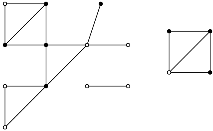
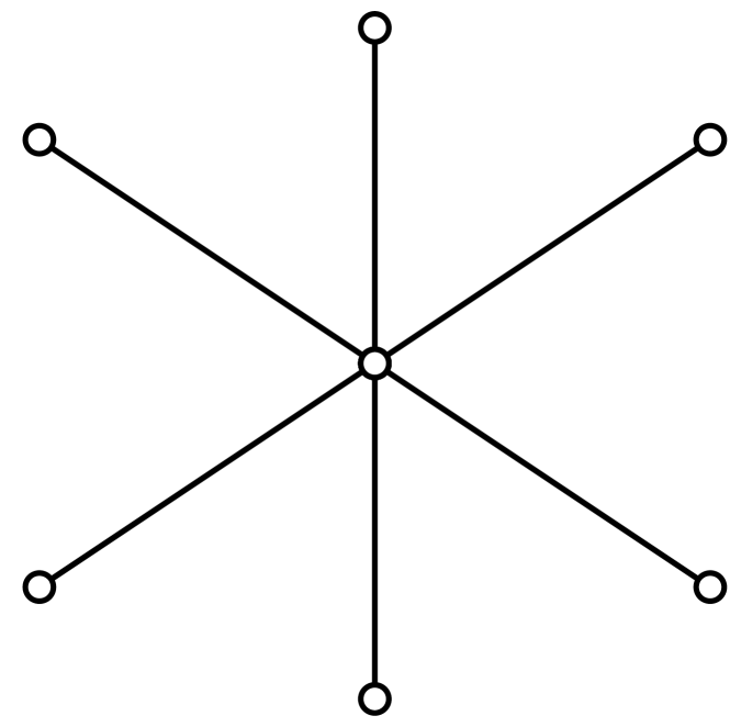
To fix notations, let $G=(V,E)$ be a simple, undirected graph on $N$ vertices. In the subgraph sampling model, we sample a set of vertices denoted by $S\subset V$, and observe their induced subgraph, denoted by $G[S]=(S,E[S])$, where the edge set is defined as $E[S]=\{\{i,j\}\in E:i,j\in S\}$. See Fig. 1 for an illustration. To simplify notations, we abbreviate the sampled graph $G[S]$ as ${\widetilde{G}}$.

(a) Parent graph $G$ with the set of sampled vertices $S$ shown in black.

(b) Subgraph induced by sampled vertices ${\widetilde{G}}=G[S]$. Non-sampled vertices are shown as isolated vertices.

Figure 1: Subgraph sampling.

According to how the set $S$ of sampled vertices is generated, there are two variations of the subgraph sampling model [21]:

• Uniform sampling: Exactly $n$ vertices are chosen uniformly at random without replacement from the vertex set $V$. In this case, the probability of observing a subgraph isomorphic to $H$ with ${\mathsf{v}}(H)=n$ is equal to

  $$\mathbb{P}[{\widetilde{G}}\simeq H]=\frac{\mathsf{s}(H,G)}{\binom{N}{n}}.$$ (1)

• Bernoulli sampling: Each vertex is sampled independently with probability $p$, where $p$ is called the sampling ratio. Thus, the sample size $|S|$ is distributed as $\mathrm{Bin}(N,p)$, and the probability of observing a subgraph isomorphic to $H$ is equal to

  $$\mathbb{P}[{\widetilde{G}}\simeq H]=\mathsf{s}(H,G)p^{{\mathsf{v}}(H)}(1-p)^{{\mathsf{v}}(G)-{\mathsf{v}}(H)}.$$ (2)

The relation between these two models is analogous to that between sampling without replacements and sampling with replacements. In the sublinear sampling regime where $n\ll N$, they are nearly equivalent. For technical simplicity, we focus on the Bernoulli sampling model and we refer to $n\triangleq pN$ as the effective sample size. Extensions to the uniform sampling model will be discussed in Section B.1 of Appendix B.

A number of previous work on subgraph sampling is closely related with the theory of graph limits [7], which is motivated by the so-called property testing problems in graphs [23]. According to [7, Definition 2.11], a graph parameter $f$ is “testable” if for any $\epsilon>0$, there exists a sample size $n$ such that for any graph $G$ with at least $n$ vertices, there is an estimator $\widehat{f}=\widehat{f}({\widetilde{G}})$ such that $\mathbb{P}[|f(G)-\widehat{f}|>\epsilon]<\epsilon$. In other words, testable properties can be estimated with sample complexity that is independent of the size of the graph. Examples of testable properties include the edge density ${\mathsf{e}}(G)/\binom{{\mathsf{v}}(G)}{2}$ and the density of maximum cuts $\frac{\mathsf{MaxCut}(G)}{{\mathsf{v}}(G)^{2}}$, where $\mathsf{MaxCut}(G)$ is the size of the maximum edge cut-set in $G$ [24]; however, the number of connected components $\mathsf{cc}(G)$ or its normalized version $\frac{\mathsf{cc}(G)}{{\mathsf{v}}(G)}$ are not testable. Instead, our focus is to understand the dependency of sample complexity of estimating $\mathsf{cc}(G)$ on the graph size $N$ as well as other graph parameters. It turns out for certain classes of graphs, the sample complexity grows sublinearly in $N$, which is the most interesting regime.

2.2 Classes of graphs

Before introducing the classes of graphs we consider in this paper, we note that, unless further structures are assumed about the parent graph, estimating many graph properties, including the number of connected components, has very high sample complexity that scales linearly with the size of the graph. Indeed, there are two main obstacles in estimating the number of connected components in graphs, namely, high-degree vertices and long induced cycles. If either is allowed to be present, we will show that even if we sample a constant faction of the vertices, any estimator of $\mathsf{cc}(G)$ has a worst-case additive error that is almost linear in the network size $N$. Specifically,

• For any sampling ratio $p$ bounded away from $1$, as long as the maximum degree is allowed to scale as $\Omega(N)$, even if we restrict the parent graph to be acyclic, the worst-case estimation error for any estimator is $\Omega(N)$.

• For any sampling ratio $p$ bounded away from $1/2$, as long as the length of the induced cycles is allowed to be $\Omega(\log N)$, even if we restrict the parent graph to have maximum degree 2, the worst-case estimation error for any estimator is $\Omega(\frac{N}{\log N})$.

The precise statements follow from the minimax lower bounds in Theorem 14 and Theorem 13 of Appendix B. Below we provide an intuitive explanation for each scenario.

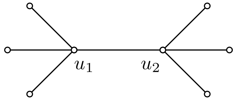
For the first claim involving large degree, consider a pair of acyclic graphs $G$ and $G^{\prime}$, where $G$ is the star graph on $N$ vertices and $G^{\prime}$ consisting of $N$ isolated vertices. Note that as long as the center vertex in $G$ is not sampled, the sampling distributions of $G$ and $G^{\prime}$ are identical. This implies that the total variation between the sampled graph under $G$ and $G^{\prime}$ is at most $p$. Since the numbers of connected components in $G$ and $G^{\prime}$ differ by $N-1$, this leads to a minimax lower bound for the estimation error of $\Omega(N)$ whenever $p$ is bounded away from one.

The effect of long induced cycles is subtler. The key observation is that a cycle and a path (or a cycle versus two cycles) locally look exactly the same. Indeed, let $G$ (resp. $G^{\prime}$) consists of $N/(2r)$ disjoint copies of the smaller graph $H$ (resp. $H^{\prime}$), where $H$ is a cycle of length $2r$ and $H^{\prime}$ consists of two disjoint cycles of length $r$. Both $G$ and $G^{\prime}$ have maximum degree $2$ and contain induced cycles of length at most $2r$. The local structure of $G$ and $G^{\prime}$ is the same (e.g., each connected subgraph with at most $r-1$ vertices appears exactly $N$ times in each graph) and the sampled versions of $H$ and $H^{\prime}$ are identically distributed provided at most $r-1$ vertices are sampled. Thus, we must sample at least $r$ vertices (which occurs with probability at most $e^{-r(1-2p)^{2}}$) for the distributions to be different. By a union bound, it can be shown that the total variation between the sampled graphs ${\widetilde{G}}$ and ${\widetilde{G}}^{\prime}$ is $O((N/r)e^{-r(1-2p)^{2}})$. Thus, whenever the sampling ratio $p$ is bounded away from $1/2$, choosing $r=\Theta(\log N)$ leads to a near-linear lower bound $\Omega(\frac{N}{\log N})$.

The difficulties caused by high-degree vertices and long induced cycles motivate us to consider classes of graphs defined by two key parameters, namely, the maximum degree $d$ and the length of the longest induced cycles $c$. The case of $c=2$ corresponds to forests (acyclic graphs), which have been considered by Frank [21]. The case of $c=3$ corresponds to chordal graphs, i.e., graphs without induced cycle of length four or above, which is the focus of this paper. It is well-known that various computation tasks that are intractable in the worst case, such as maximal clique and graph coloring, are easy for chordal graphs; it turns out that the chordality structure also aids in both the design and the analysis of computationally efficient estimators which provably attain the optimal sample complexity.

3 Main results

This section summarizes our main results in terms of the minimax risk of estimating the number of connected components over various class of graphs. As mentioned before, for ease of exposition, we focus on the Bernoulli sampling model, where each vertex is sampled independently with probability $p$. Similar conclusions can be obtained for the uniform sampling model upon identifying $p=n/N$, as given in Section B.1.

When $p$ grows from $0$ to $1$, an increasing fraction of the graph is observed and intuitively the estimation problem becomes easier. Indeed, all forthcoming minimax rates are inversely proportional to powers of $p$. Of particular interest is whether accurate estimation in the sublinear sampling regime, i.e., $p=o(1)$. The forthcoming theory will give explicit conditions on $p$ for this to hold true.

As mentioned in the previous section, the main class of graphs we study is the so-called chordal graphs (see Fig. 2 for an example):

Definition 1.

A graph $G$ is chordal if it does not contain induced cycles of length four or above, i.e., $\mathsf{s}(C_{k},G)=0$ for $k\geq 4$.

(a) Chordal graph.

(b) Non-chordal graph (containing an induced $C_{4}$).

Figure 2: Examples of chordal and non-chordal graphs both with three connected components.

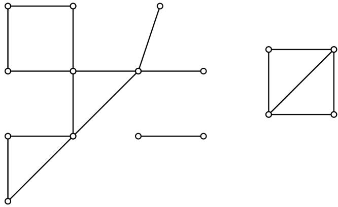
We emphasize that chordal graphs are allowed to have arbitrarily long cycles but no induced cycles longer than three. The class of chordal graphs encompasses forests and disjoint union of cliques as special cases, the two models that were studied in Frank’s original paper [21]. In addition to constructing estimators that adapt to larger collections of graphs (for which forests and unions of cliques are special cases), we also provide theoretical analysis and optimality guarantees – elements that were not considered in past work.

Next, we characterize the rate of the minimax mean-squared error for estimating the number of connected components in a chordal graph, which turns out to depend on the number of vertices, the maximum degree, and the clique number. The upper and lower bounds differ by at most a multiplicative factor depending only on the clique number. To simplify the notation, henceforth we denote $q=1-p$.

Theorem 1 (Chordal graphs).

Let ${\mathcal{G}}(N,d,\omega)$ denote the collection of all chordal graphs on $N$ vertices with maximum degree and clique number at most $d$ and $\omega\geq 2$, respectively. Then

$$\inf_{\widehat{\mathsf{cc}}}\sup_{G\in{\mathcal{G}}(N,d,\omega)}\mathbb{E}_{G}|\widehat{\mathsf{cc}}-\mathsf{cc}(G)|^{2}=\Theta_{\omega}\left(\left(\frac{N}{p^{\omega}}\vee\frac{Nd}{p^{\omega-1}}\right)\wedge N^{2}\right),$$

where the lower bound holds provided that $p\leq p_{0}$ for some constant $p_{0}<\frac{1}{2}$ that only depends on $\omega$. Furthermore, if $p\geq 1/2$, then for any $\omega$,

$$\inf_{\widehat{\mathsf{cc}}}\sup_{G\in{\mathcal{G}}(N,d,\omega)}\mathbb{E}_{G}|\widehat{\mathsf{cc}}-\mathsf{cc}(G)|^{2}\leq Nq(d+1).$$ (3)

Specializing Theorem 1 to $\omega=2$ yields the minimax rates for estimating the number of trees in forests for small sampling ratio $p$. The next theorem shows that the result holds verbatim even if $p$ is arbitrarily close to 1, and, consequently, shows minimax rate-optimality of the bound in (3). The lower bound component is proved in Section B.3 of Appendix B.

Theorem 2 (Forests).

Let $\mathcal{F}(N,d)\triangleq{\mathcal{G}}(N,d,2)$ denote the collection of all forests on $N$ vertices with maximum degree at most $d$. Then for all $0\leq p\leq 1$ and $1\leq d\leq N$,

$$\inf_{\widehat{\mathsf{cc}}}\sup_{G\in\mathcal{F}(N,d)}\mathbb{E}_{G}|\widehat{\mathsf{cc}}-\mathsf{cc}(G)|^{2}\asymp\left(\frac{Nq}{p^{2}}\vee\frac{Nqd}{p}\right)\wedge N^{2}.$$ (4)

The upper bounds in the previous results are achieved by unbiased estimators. As (3) shows, they work well even when the clique number $\omega$ grow with $N$, provided we sample more than half of the vertices; however, if the sample ratio $p$ is below $\frac{1}{2}$, especially in the sublinear regime of $p=o(1)$ that we are interested in, the variance is exponentially large. To deal with large $d$ and $\omega$, we must give up unbiasedness to achieve a good bias-variance tradeoff. Such biased estimators, obtained using the smoothing technique introduced in [47], lead to better performance as quantified in the following theorem. The proofs of these bounds are given in Theorem 7 and Theorem 9.

Theorem 3 (Chordal graphs).

Let ${\mathcal{G}}(N,d)$ denote the collection of all chordal graphs on $N$ vertices with maximum degree at most $d$. Then, for any $p<1/2$,

$$\inf_{\widehat{\mathsf{cc}}}\sup_{G\in{\mathcal{G}}(N,d)}\mathbb{E}_{G}|\widehat{\mathsf{cc}}-\mathsf{cc}(G)|^{2}\lesssim N^{2}\left(N/d^{2}\right)^{-\frac{p}{2-3p}}.$$

Finally, for the special case of graphs consisting of disjoint union of cliques, as the following theorem shows, there are enough structures so that we no longer need to impose any condition on the maximal degree. Similar to Theorem 3, the achievable scheme is a biased estimator, significantly improving the unbiased estimator in [27, 21] which has exponentially large variance.

Theorem 4 (Cliques).

Let ${\mathcal{C}}(N)$ denote the collection of all graphs on $N$ vertices consisting of disjoint unions of cliques. Then, for any $p<1/2$,

$$\inf_{\widehat{\mathsf{cc}}}\sup_{G\in{\mathcal{C}}(N)}\mathbb{E}_{G}|\widehat{\mathsf{cc}}-\mathsf{cc}(G)|^{2}\leq N^{2}(N/4)^{-\frac{p}{2-3p}}.$$

Alternatively, the above results are summarized in Table 1 in terms of the sample complexity, i.e., the minimum sample size that allows an estimator $\mathsf{cc}(G)$ within an additive error of $\epsilon N$ with probability, say, at least 0.99, uniformly for all graphs in a given class. Here the sample size is understood as the average number of sampled vertices $n=pN$. We have the following characterization:

Graph	Sample complexity $n$
Chordal	$\Theta_{\omega}\left(\max\left\{N^{\frac{\omega-2}{\omega-1}}{d}^{\frac{1}{\omega-1}}\epsilon^{-\frac{2}{\omega-1}},\;N^{\frac{\omega-1}{\omega}}\epsilon^{-\frac{2}{\omega}}\right\}\right)$
Forest	$\Theta\left(\max\left\{\frac{d}{\epsilon^{2}},\;\frac{\sqrt{N}}{\epsilon}\right\}\right)$
Cliques	$\Theta\left(\frac{N}{\log N}\log\frac{1}{\epsilon}\right)$,  $\epsilon\geq N^{-1/2+\Omega(1)}$ *

• The lower bound part of this statement follows from [58, Section 3], which shows the optimality of Theorem 4.

Table 1: Sample complexity for various classes of graphs

A consequence of Theorem 2 is that if the effective sample size $n$ scales as $O(\max(\sqrt{N},d))$, for the class of forests $\mathcal{F}(N,d)$ the worse-case estimation error for any estimator is $\Omega(N)$, which is within a constant factor to the trivial error bound when no samples are available. Conversely, if $n\gg\max(\sqrt{N},d)$, which is sublinear in $N$ as long as the maximal degree satisfies $d=o(N)$, then it is possible to achieve a non-trivial estimation error of $o(N)$. More generally for chordal graphs, Theorem 1 implies that if $n=O(\max(N^{\frac{\omega-1}{\omega}},d^{\frac{1}{\omega-1}}N^{\frac{\omega-2}{\omega-1}}))$, the worse-case estimation error in ${\mathcal{G}}(N,d,\omega)$ for any estimator is at least $\Omega_{\omega}(N)$,

4 Algorithms and performance guarantees

In this section we propose estimators which provably achieve the upper bounds presented in Section 3 for the Bernoulli sampling model. In Section 4.1, we highlight some combinatorial properties and characterizations of chordal graphs that underpin both the construction and the analysis of the estimators in Section 4.2. The special case of disjoint unions of cliques is treated in Section 4.3, where the estimator of Frank [21] is recovered and further improved. Analogous results for the uniform sampling model are given in Section B.1 of Appendix B. Finally, in Section 4.4, we discuss a heuristic to generalize the methodology to non-chordal graphs.

4.1 Combinatorial properties of chordal graphs

In this subsection we discuss the relevant combinatorial properties of chordal graphs which aid in the design and analysis of our estimators. We start by introducing a notion of vertex elimination ordering.

Definition 2.

A perfect elimination ordering (PEO) of a graph $G$ on $N$ vertices is a vertex labelling $\{v_{1},v_{2},\dots,v_{N}\}$ such that, for each $j$, $N_{G}(v_{j})\cap\{v_{1},...,v_{j-1}\}$ is a clique.

Figure 3: A chordal graph $G$ with PEO labelled. In this example, $\mathsf{cc}(G)=3=16-19+6=\mathsf{s}(K_{1},G)-\mathsf{s}(K_{2},G)+\mathsf{s}(K_{3},G)$.

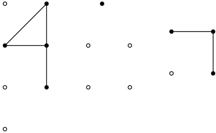
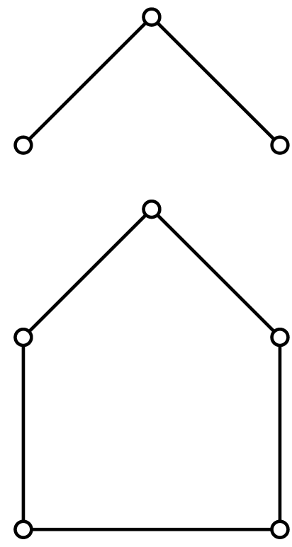
In other words, if one eliminates the vertices sequentially according to a PEO starting from the last vertex, at each step, the neighborhood of the vertex to be eliminated forms a clique; see Fig. 3 for an example. A classical result of Dirac asserts that the existence of a PEO is in fact the defining property of chordal graphs (cf. e.g., [56, Theorem 5.3.17]).

Theorem 5.

A graph is chordal if and only if it admits a PEO.

In general a PEO of a chordal graph is not unique; however, it turns out that the size of each neighborhood in the vertex elimination process is unique up to permutation, a fact that we will exploit later on. The next lemma makes this claim precise. For brevity, we defer its proof to Appendix A.

Lemma 1.

Let $\{v_{1},\dots,v_{N}\}$ and $\{v^{\prime}_{1},\dots,v^{\prime}_{N}\}$ be two PEOs of a chordal graph $G$. Let ${\mathsf{c}}_{j}$ and ${\mathsf{c}}^{\prime}_{j}$ denote the cardinalities of $N_{G}(v_{j})\cap\{v_{1},\dots,v_{j-1}\}$ and $N_{G}(v^{\prime}_{j})\cap\{v^{\prime}_{1},\dots,v^{\prime}_{j-1}\}$, respectively. Then there is a bijection $\sigma:[N]\to[N]$ such that ${\mathsf{c}}_{\sigma(j)}={\mathsf{c}}^{\prime}_{j}$ for all $j$.

Recall that $\mathsf{s}(K_{i},G)$ denotes the number of cliques of size $i$ in $G$. For any chordal graph $G$, it turns out that the number of components can be expressed as an alternating sum of clique counts (cf. e.g., [56, Exercise 5.3.22, p. 231]); see Fig. 3 for an example. Instead of the topological proof involving properties of the clique simplex of chordal graphs [44, 14], in the next lemma we provide a combinatorial proof together with a sandwich bound. The main purpose of this exposition is to explain how to enumerate cliques in chordal graphs using vertex elimination, which plays a key role in analyzing the statistical estimator developed in the next subsection.

Lemma 2.

For any chordal graph $G$,

$$\mathsf{cc}(G)=\sum_{i\geq 1}(-1)^{i+1}\mathsf{s}(K_{i},G).$$ (5)

Furthermore, for any $r\geq 1$,

$$\sum_{i=1}^{2r}(-1)^{i+1}\mathsf{s}(K_{i},G)\leq\mathsf{cc}(G)\leq\sum_{i=1}^{2r-1}(-1)^{i+1}\mathsf{s}(K_{i},G).$$ (6)

Proof.

Since $G$ is chordal, by Theorem 5, it has a PEO $\{v_{1},\dots,v_{N}\}$. Define

$$C_{j}\triangleq N_{G}(v_{j})\cap\{v_{1},\ldots,v_{j-1}\},\quad{\mathsf{c}}_{j}\triangleq|C_{j}|.$$ (7)

Since the neighbors of $v_{j}$ among $v_{1},\dots,v_{j-1}$ form a clique, we obtain $\binom{{\mathsf{c}}_{j}}{i-1}$ new cliques of size $i$ when we adjoin the vertex $v_{j}$ to the subgraph induced by $v_{1},\dots,v_{j-1}$. Thus,

$$\mathsf{s}(K_{i},G)=\sum_{j=1}^{N}\binom{{\mathsf{c}}_{j}}{i-1}.$$ (8)

Moreover, note that $\mathsf{cc}(G)=\sum_{j=1}^{N}\mathbbm{1}\{{\mathsf{c}}_{j}=0\}$. Hence, it follows that

$$\sum_{i=1}^{2r-1}(-1)^{i+1}\mathsf{s}(K_{i},G) =\sum_{i=1}^{2r-1}(-1)^{i+1}\sum_{j=1}^{N}\binom{{\mathsf{c}}_{j}}{i-1}=\sum_{j=1}^{N}\sum_{i=1}^{2r-1}(-1)^{i+1}\binom{{\mathsf{c}}_{j}}{i-1}$$

$$=\sum_{j=1}^{N}\sum_{i=0}^{2(r-1)}(-1)^{i}\binom{{\mathsf{c}}_{j}}{i}=\sum_{j=1}^{N}\left(\binom{{\mathsf{c}}_{j}-1}{2(r-1)}\mathbbm{1}\{{\mathsf{c}}_{j}\neq 0\}+\mathbbm{1}\{{\mathsf{c}}_{j}=0\}\right)$$

$$\geq\sum_{j=1}^{N}\mathbbm{1}\{{\mathsf{c}}_{j}=0\}=\mathsf{cc}(G),$$

and

$$\sum_{i=1}^{2r}(-1)^{i+1}\mathsf{s}(K_{i},G) =\sum_{i=1}^{2r}(-1)^{i+1}\sum_{j=1}^{N}\binom{{\mathsf{c}}_{j}}{i-1}=\sum_{j=1}^{N}\sum_{i=1}^{2r}(-1)^{i+1}\binom{{\mathsf{c}}_{j}}{i-1}$$

$$=\sum_{j=1}^{N}\sum_{i=0}^{2r-1}(-1)^{i}\binom{{\mathsf{c}}_{j}}{i}=\sum_{j=1}^{N}\left(-\binom{{\mathsf{c}}_{j}-1}{2r-1}\mathbbm{1}\{{\mathsf{c}}_{j}\neq 0\}+\mathbbm{1}\{{\mathsf{c}}_{j}=0\}\right)$$

$$\leq\sum_{j=1}^{N}\mathbbm{1}\{{\mathsf{c}}_{j}=0\}=\mathsf{cc}(G).\qed$$

4.2 Estimators for chordal graphs

4.2.1 Bounded clique number: unbiased estimators

In this subsection, we consider unbiased estimation of the number of connected components in chordal graphs. As we will see, unbiased estimators turn out to be minimax rate-optimal for chordal graphs with bounded clique size. The subgraph count identity (5) suggests the following unbiased estimator

$$\widehat{\mathsf{cc}}=-\sum_{i\geq 1}\left(-\frac{1}{p}\right)^{i}\mathsf{s}(K_{i},{\widetilde{G}}).$$ (9)

Indeed, since the probability of observing any given clique of size $i$ is $p^{i}$, (9) is clearly unbiased in the same spirit of the Horvitz-Thompson estimator [33]. In the case where the parent graph $G$ is a forest, (9) reduces to the estimator $\widehat{\mathsf{cc}}={\mathsf{v}}({\widetilde{G}})/p-{\mathsf{e}}({\widetilde{G}})/p^{2}$, as proposed by Frank [21].

A few comments about the estimator (9) are in order. First, it is completely adaptive to the parameters $\omega$, $d$ and $N$, since the sum in (9) terminates at the clique number of the subsampled graph. Second, it can be evaluated in time that is linear in ${\mathsf{v}}(\widetilde{G})+{\mathsf{e}}(\widetilde{G})$. Indeed, the next lemma gives a simple formula for computing (9) using the PEO. Since a PEO of a chordal graph $G$ can be found in $O({\mathsf{v}}(G)+{\mathsf{e}}(G))$ time [50, 54] and any induced subgraph of a chordal graph remains chordal, the estimator (9) can be evaluated in linear time. Recall that $q=1-p$.

Lemma 3.

Let $\{\widetilde{v}_{1},\dots,\widetilde{v}_{m}\}$, $m=|S|$, be a PEO of ${\widetilde{G}}$. Then

$$\widehat{\mathsf{cc}}=\frac{1}{p}\sum_{j=1}^{m}\left(-\frac{q}{p}\right)^{\widetilde{{\mathsf{c}}}_{j}},$$ (10)

where $\widetilde{{\mathsf{c}}}_{j}\triangleq|N_{{\widetilde{G}}}(\widetilde{v}_{j})\cap\{\widetilde{v}_{1},\dots,\widetilde{v}_{j-1}\}|$ can be calculated from ${\widetilde{G}}$ in linear time.

Proof.

Because the subsampled graph ${\widetilde{G}}$ is also chordal, by (8), we have $\mathsf{s}(K_{i},{\widetilde{G}})=\sum_{j=1}^{m}\binom{\widetilde{{\mathsf{c}}}_{j}}{i-1}$. Thus, (9) can also be written as

$$\widehat{\mathsf{cc}} =-\sum_{i=1}^{m}\left(-\frac{1}{p}\right)^{i}\mathsf{s}(K_{i},{\widetilde{G}})=-\sum_{i=1}^{m}\left(-\frac{1}{p}\right)^{i}\sum_{j=1}^{m}\binom{\widetilde{{\mathsf{c}}}_{j}}{i-1}$$

$$=-\sum_{j=1}^{m}\sum_{i=1}^{m}\left(-\frac{1}{p}\right)^{i}\binom{\widetilde{{\mathsf{c}}}_{j}}{i-1}=\frac{1}{p}\sum_{j=1}^{m}\sum_{i=0}^{m-1}\left(-\frac{1}{p}\right)^{i}\binom{\widetilde{{\mathsf{c}}}_{j}}{i}$$

$$=\frac{1}{p}\sum_{j=1}^{m}\left(-\frac{q}{p}\right)^{\widetilde{{\mathsf{c}}}_{j}}.\qed$$

In addition to the aforementioned computational advantages of using (10) over (9), let us also describe why (10) is more numerically stable. Both estimators are equal to an alternating sum of the form $\sum_{i}a_{i}(-1/p)^{b_{i}}$. In (10), $a_{i}=q^{b_{i}}/p$, whereas $a_{i}=-\mathsf{s}(K_{b_{i}},{\widetilde{G}})$ in (9), which can be as large as $O(N2^{\omega})$ in magnitude. Thus, when ${\widetilde{G}}$ is sufficiently dense, computation of (9) involves adding and subtracting extremely large numbers – making it prone to integer overflow and suffer from loss of numerical precision. For example, double-precision floating-point arithmetic (e.g., used in R) gives from $15$ to $17$ significant decimal digits precision. In our experience, this tends to be insufficient for most mid-sized, real-world networks (see Appendix C) and the estimator (9) outputs wildly imprecise numbers.

Using elementary enumerative combinatorics, in particular, the vertex elimination structure of chordal graphs, the next theorem provides a performance guarantee for the estimator (9) in terms of a variance bound and a high-probability bound, which, in particular, settles the upper bound of the minimax mean squared error in Theorem 1 and Theorem 2.

Theorem 6.

Let $G$ be a chordal graph on $N$ vertices with maximum degree and clique number at most $d$ and $\omega\geq 2$, respectively. Suppose ${\widetilde{G}}$ is generated by the $\mathrm{Bern}(p)$ sampling model. Then $\widehat{\mathsf{cc}}$ defined in (9) is an unbiased estimator of $\mathsf{cc}(G)$. Furthermore,

$$\mathsf{Var}[\widehat{\mathsf{cc}}]\leq N\left(\frac{q}{p}+d\right)\left(\left(\frac{q}{p}\right)^{\omega-1}\vee\frac{q}{p}\right)\leq\frac{N}{p^{\omega}}+\frac{Nd}{p^{\omega-1}},$$ (11)

and for all $t\geq 0$,

$$\mathbb{P}\left[|\widehat{\mathsf{cc}}-\mathsf{cc}(G)|\geq t\right]\leq 2\exp\left\{-\frac{8p^{\omega}t^{2}}{25(d\omega+1)(N+t/3)}\right\}.$$ (12)

To prove Theorem 6 we start by presenting a useful lemma. Note that Lemma 3 states that $\widehat{\mathsf{cc}}$ is a linear combination of $(-q/p)^{\widetilde{{\mathsf{c}}}_{j}}$; here $\widetilde{{\mathsf{c}}}_{j}$ is computed using a PEO of the sampled graph, which itself is random. The next result allows us rewrite the same estimator as a linear combination of $(-q/p)^{\widehat{{\mathsf{c}}}_{j}}$, where $\widehat{{\mathsf{c}}}_{j}$ depends on the PEO of the parent graph (which is deterministic). Note that this is only used in the course of analysis since the population level PEO is not observed. This representation is extremely useful in analyzing the performance of $\widehat{\mathsf{cc}}$ and its biased variant in Section 4.2.2. More generally, we have the following result, which we prove in Appendix A.

Lemma 4.

Let $\{v_{1},\dots,v_{N}\}$ be a PEO of $G$ and let $\{\widetilde{v}_{1},\dots,\widetilde{v}_{m}\}$, $m=|S|$, be a PEO of ${\widetilde{G}}$. Furthermore, let $\widehat{{\mathsf{c}}}_{j}=|N_{{\widetilde{G}}}(v_{j})\cap\{v_{1},\dots,v_{j-1}\}|$ and $\widetilde{{\mathsf{c}}}_{j}=|N_{{\widetilde{G}}}(\widetilde{v}_{j})\cap\{\widetilde{v}_{1},\dots,\widetilde{v}_{j-1}\}|$. Let $\widehat{{\mathsf{g}}}=\widehat{{\mathsf{g}}}({\widetilde{G}})$ be a linear estimator of the form

$$\widehat{{\mathsf{g}}}=\sum_{j=1}^{m}g(\widetilde{{\mathsf{c}}}_{j}).$$ (13)

Then

$$\widehat{{\mathsf{g}}}=\sum_{j=1}^{N}b_{j}g(\widehat{{\mathsf{c}}}_{j}),$$

where $b_{j}\triangleq\mathbbm{1}\left\{{v_{j}\in S}\right\}$.

We also need a couple of ancillary results whose proofs are also given in Appendix A:

Lemma 5 (Orthogonality).

Let

$$f(k)=\left(-\frac{q}{p}\right)^{k},\quad k\geq 0.$$ (14)

Let $\{b_{v}:v\in V\}$ be independent $\mathrm{Bern}(p)$ random variables. For any $S\subset V$, define $N_{S}=\sum_{v\in S}b_{v}$. Then

$$\mathbb{E}[f(N_{S})f(N_{T})]=\mathbbm{1}\{S=T\}(q/p)^{|{S}|}.$$

In particular, $\mathbb{E}[f(N_{S})]=0$ for any $S\neq\emptyset$.

Lemma 6.

Let $\{v_{1},\ldots,v_{N}\}$ be a PEO of a chordal graph $G$ on $N$ vertices with maximum degree and clique number at most $d$ and $\omega$, respectively. Let $C_{j}\triangleq N_{G}(v_{j})\cap\{v_{1},\ldots,v_{j-1}\}$. Then

$$|\{(i,j):i\neq j,\;C_{j}=C_{i}\neq\emptyset\}|\leq N(d-1).$$ (15)

Furthermore, let

$$A_{j}=\{v_{j}\}\cup C_{j}.$$ (16)

Then for each $j\in[N]$,

$$|\{i\in[N]:i\neq j,\;A_{i}\cap A_{j}\neq\emptyset\}|\leq d\omega.$$ (17)

Proof of Theorem 6.

For a chordal graph $G$ on $N$ vertices, let $\{v_{1},\dots,v_{N}\}$ be a PEO of $G$. Recall from (7) that $C_{j}$ denote the set of neighbors of $v_{j}$ among $v_{1},\dots,v_{j-1}$ and ${\mathsf{c}}_{j}$ denotes its cardinality. That is,

$${\mathsf{c}}_{j}=|N_{G}(v_{j})\cap\{v_{1},\ldots,v_{j-1}\}|=\sum_{k=1}^{j-1}\mathbbm{1}\{v_{k}\sim v_{j}\}.$$

As in Lemma 4, let $\widehat{{\mathsf{c}}}_{j}$ denote the sample version, i.e.,

$$\widehat{{\mathsf{c}}}_{j}\triangleq|N_{{\widetilde{G}}}(v_{j})\cap\{v_{1},\ldots,v_{j-1}\}|=b_{j}\sum_{k=1}^{j-1}b_{k}\mathbbm{1}\{v_{k}\sim v_{j}\},$$

where $b_{k}\triangleq\mathbbm{1}\{v_{k}\in S\}{\stackrel{{\scriptstyle\text{i.i.d.}}}{{\sim}}}\mathrm{Bern}(p)$. By Lemma 3 and Lemma 4, $\widehat{\mathsf{cc}}$ can be written as

$$\widehat{\mathsf{cc}}=\frac{1}{p}\sum_{j=1}^{m}f(\widetilde{{\mathsf{c}}}_{j})=\frac{1}{p}\sum_{j=1}^{N}b_{j}f(\widehat{{\mathsf{c}}}_{j}),$$ (18)

where the function $f$ is defined in (14).

To show the variance bound (11), we note that

$$\mathsf{Var}[\widehat{\mathsf{cc}}]=\frac{1}{p^{2}}\sum_{j=1}^{N}\mathsf{Var}[b_{j}f(\widehat{{\mathsf{c}}}_{j})]+\frac{1}{p^{2}}\sum_{j\neq i}\mathsf{Cov}[b_{j}f(\widehat{{\mathsf{c}}}_{j}),b_{i}f(\widehat{c}_{i})].$$ (19)

Note that $\widehat{{\mathsf{c}}}_{j}\mid\{b_{j}=1\}\sim\mathrm{Bin}({\mathsf{c}}_{j},p)$. Using Lemma 5, it is straightforward to verify that

$$\mathsf{Var}[b_{j}f(\widehat{{\mathsf{c}}}_{j})]=\begin{cases}p\left(\frac{q}{p}\right)^{{\mathsf{c}}_{j}}&\text{if }{\mathsf{c}}_{j}>0\\ pq&\text{if }{\mathsf{c}}_{j}=0\end{cases}.$$ (20)

Since ${\mathsf{c}}_{j}\leq\omega-1$, it follows that

$$\mathsf{Var}[b_{j}f(\widehat{{\mathsf{c}}}_{j})]\leq p\left[\left(\frac{q}{p}\right)^{\omega-1}\vee\frac{q}{p}\right].$$ (21)

The covariance terms are less obvious to bound; but thanks to the orthogonality property in Lemma 5, many of them are zero or negative. Let $N_{C}\triangleq\sum b_{j}\mathbbm{1}\left\{{v_{j}\in C}\right\}$. For any $j$, since $v_{j}\not\in C_{j}$ by definition, applying Lemma 5 yields

$$\mathbb{E}[b_{j}f(\widehat{{\mathsf{c}}}_{j})]=p\mathbb{E}[f(N_{C_{j}})]=p\mathbbm{1}\left\{{C_{j}=\emptyset}\right\}.$$ (22)

Without loss of generality, assume $j<i$. By the definition of $C_{j}$, we have $v_{i}\notin C_{j}$. Next, we consider two cases separately:

Case I: $v_{j}\notin C_{i}$.

If either $C_{j}$ or $C_{i}$ is nonempty, Lemma 5 yields

$$\mathsf{Cov}[b_{j}f(\widehat{{\mathsf{c}}}_{j}),b_{i}f(\widehat{{\mathsf{c}}}_{i})]\overset{(\ref{eq:dec})}{=}\mathbb{E}[b_{i}b_{j}f(\widehat{{\mathsf{c}}}_{j})f(\widehat{{\mathsf{c}}}_{i})]=p^{2}\mathbb{E}[f(N_{C_{j}})f(N_{C_{i}})]=p^{2}\mathbbm{1}\{C_{j}=C_{i}\}\left(\frac{q}{p}\right)^{{\mathsf{c}}_{j}}.$$

If $C_{j}=C_{i}=\emptyset$, then $\mathsf{Cov}[b_{j}f(\widehat{{\mathsf{c}}}_{j}),b_{i}f(\widehat{{\mathsf{c}}}_{i})]=\mathsf{Cov}[b_{j},b_{i}]=0$.

Case II: $v_{j}\in C_{i}$.

Then $\mathbb{E}[b_{i}f(\widehat{{\mathsf{c}}}_{i})]=0$ by (22). Using Lemma 5 again, we have

$$\mathsf{Cov}[b_{j}f(\widehat{{\mathsf{c}}}_{j}),b_{i}f(\widehat{{\mathsf{c}}}_{i})] =p\mathbb{E}\left[b_{j}\left(-\frac{q}{p}\right)^{b_{j}}\right]\mathbb{E}[f(N_{C_{j}})f(N_{C_{i}\setminus\{v_{j}\}})]$$

$$=-pq\mathbb{E}[f(N_{C_{j}})f(N_{C_{i}\setminus\{v_{j}\}})]$$

$$=-pq\mathbbm{1}\{C_{j}=C_{i}\setminus\{v_{j}\}\}\left(\frac{q}{p}\right)^{{\mathsf{c}}_{j}}.$$

To summarize, we have shown that

$$\mathsf{Cov}[b_{j}f(\widehat{{\mathsf{c}}}_{j}),b_{i}f(\widehat{{\mathsf{c}}}_{i})]=\begin{cases}p^{2}\left(\frac{q}{p}\right)^{{\mathsf{c}}_{j}}&\text{if }C_{j}=C_{i}\neq\emptyset\\ -pq\left(\frac{q}{p}\right)^{{\mathsf{c}}_{j}}&\text{if }C_{j}=C_{i}\setminus\{v_{j}\}\text{ and }v_{j}\in C_{i}\\ 0&\text{otherwise}\end{cases}.$$

Thus,

$$\sum_{j\neq i}\mathsf{Cov}[b_{j}f(\widehat{{\mathsf{c}}}_{j}),b_{i}f(\widehat{c}_{i})]\leq\sum_{j\neq i:\;C_{j}=C_{i}\neq\emptyset}p^{2}\left(\frac{q}{p}\right)^{{\mathsf{c}}_{j}}\overset{(\ref{eq:Cjnumber})}{\leq}N(d-1)p^{2}\left[\left(\frac{q}{p}\right)^{\omega-1}\vee\frac{q}{p}\right].$$ (23)

Finally, combining (19), (21) and (23) yields the desired (11).

The high-probability bound (12) for $\widehat{\mathsf{cc}}$ follows from the concentration inequality in Lemma 10 in Appendix A. To apply this result, note that $\widehat{\mathsf{cc}}$ is a sum of dependent random variables

$$\widehat{\mathsf{cc}}=\sum_{j\in[N]}Y_{j},$$ (24)

where $Y_{j}=\frac{1}{p}b_{j}f(\widehat{{\mathsf{c}}}_{j})$ satisfies $\mathbb{E}[Y_{j}]=0$ for ${\mathsf{c}}_{j}>0$ and $|Y_{j}|\leq b\triangleq(\frac{1}{p})^{\omega}$ almost surely. Also, $S\triangleq\sum_{j\in[N]}\mathsf{Var}[Y_{j}]\leq N(\frac{1}{p})^{\omega}$ by (20). To control the dependency between $\{Y_{j}\}_{j\in[N]}$, note that $\widehat{{\mathsf{c}}}_{j}=b_{j}\sum_{k:v_{k}\in C_{j}}b_{k}$. Thus $Y_{j}$ only depends on $\{b_{k}:k\in A_{j}\}$, where $A_{j}=\{v_{j}\}\cup C_{j}$. Define a dependency graph $\Gamma$, where $V(\Gamma)=[N]$ and

$$E(\Gamma)=\{\{i,j\}:i\neq j,\;A_{i}\cap A_{j}\neq\emptyset\}.$$

Then $\Gamma$ has maximum degree bounded by $d\omega$, by Lemma 6. ∎

4.2.2 Unbounded clique number: smoothed estimators

Up to this point, we have only considered unbiased estimators of the number of connected components. If the sample ratio $p$ is at least $\frac{1}{2}$, Theorem 1 implies its variance is

$$\mathsf{Var}[\widehat{\mathsf{cc}}]\leq N(d+1),$$

regardless of the clique number $\omega$ of the parent graph. However, if the clique number $\omega$ grows with $N$, for small sampling ratio $p$ the coefficients of the unbiased estimator (9) are as large as $\frac{1}{p^{\omega}}$ which results in exponentially large variance. Therefore, in order to deal with graphs with large cliques, we must give up unbiasedness to achieve better bias-variance tradeoff. Using a technique known as smoothing introduced in [47], next we modify the unbiased estimator to achieve a good bias-variance tradeoff.

To this end, consider a discrete random variable $L\in\mathbb{N}$ independent of everything else. Define the following estimator by discarding those terms in (10) for which $\widetilde{{\mathsf{c}}}_{j}$ exceeds $L$, and then averaging over the distribution of $L$. In other words, let

$$\widehat{\mathsf{cc}}_{L}\triangleq\mathbb{E}_{L}\left[\frac{1}{p}\sum_{j=1}^{m}\left(-\frac{q}{p}\right)^{\widetilde{{\mathsf{c}}}_{j}}\mathbbm{1}\{\widetilde{{\mathsf{c}}}_{j}\leq L\}\right]=\frac{1}{p}\sum_{j=1}^{m}\left(-\frac{q}{p}\right)^{\widetilde{{\mathsf{c}}}_{j}}\mathbb{P}\left[L\geq\widetilde{{\mathsf{c}}}_{j}\right].$$ (25)

Effectively, smoothing acts as soft truncation by introducing a tail probability that modulates the exponential growth of the original coefficients. The variance can then be bounded by the maximum magnitude of the coefficients in (25). Like (9), (25) can be computed in linear time.

The next theorem bounds the mean-square error of $\widehat{\mathsf{cc}}_{L}$, which implies the minimax upper bound previously announced in Theorem 3. Its proof is somewhat technical and so we defer it to Appendix A.

Theorem 7.

Let $L\sim\mathrm{Poisson}(\lambda)$ with $\lambda=\frac{p}{2-3p}\log\left(\frac{Np}{1+d\omega}\right)$. If the maximum degree and clique number of $G$ is at most $d$ and $\omega$, respectively, then when $p<1/2$,

$$\mathbb{E}_{G}|\widehat{\mathsf{cc}}_{L}-\mathsf{cc}(G)|^{2}\leq 2N^{2}\left(\frac{Np}{1+d\omega}\right)^{-\frac{p}{2-3p}}.$$

4.3 Unions of cliques

If the parent graph $G$ consists of disjoint union of cliques, so does the sampled graph ${\widetilde{G}}$. Counting cliques in each connected components, we can rewrite the estimator (9) as

$$\widehat{\mathsf{cc}}=\sum_{r\geq 1}\left(1-\left(-\frac{q}{p}\right)^{r}\right)\widetilde{\mathsf{cc}}_{r}=\mathsf{cc}({\widetilde{G}})-\sum_{r\geq 1}\left(-\frac{q}{p}\right)^{r}\widetilde{\mathsf{cc}}_{r},$$ (26)

where $\widetilde{\mathsf{cc}}_{r}$ is the number of components in the sampled graph $\widetilde{G}$ that have $r$ vertices. This coincides with the unbiased estimator proposed by Frank [21] for cliques, which is, in turn, based on the estimator of Goodman [27]. The following theorem, whose proof is given in Appendix A, provides an upper bound on its variance, recovering the previous result in [21, Corollary 11]:

Theorem 8.

Let $G$ be a disjoint union of cliques with clique number at most $\omega$. Then $\widehat{\mathsf{cc}}$ is an unbiased estimator of $\mathsf{cc}(G)$ and

$$\mathbb{E}_{G}|\widehat{\mathsf{cc}}-\mathsf{cc}(G)|^{2}=\mathsf{Var}[\widehat{\mathsf{cc}}]=\sum_{r=1}^{N}\left(\frac{q}{p}\right)^{r}\mathsf{cc}_{r}\leq N\left(\left(\frac{q}{p}\right)^{\omega}\wedge\frac{q}{p}\right),$$

where $\mathsf{cc}_{r}$ is the number of connected components in $G$ of size $r$.

Theorem 8 implies that as long as we sample at least half of the vertices, i.e., $p\geq\frac{1}{2}$, for any $G$ consisting of disjoint cliques, the unbiased estimator (26) satisfies

$$\mathbb{E}_{G}|\widehat{\mathsf{cc}}-\mathsf{cc}(G)|^{2}\leq N,$$

regardless of the clique size. However, if $p<1/2$, the variance can be exponentially large in $N$. Next, we use the smoothing technique again to obtain a biased estimator with near-optimal performance. To this end, consider a discrete random variable $L\in\mathbb{N}$ and define the following estimator by truncating (26) at the random location $L$ and average over its distribution:

$$\widetilde{\mathsf{cc}}_{L}\triangleq\mathsf{cc}({\widetilde{G}})-\mathbb{E}_{L}\left[\sum_{r=1}^{L}\left(-\frac{q}{p}\right)^{r}\widetilde{\mathsf{cc}}_{r}\right]=\mathsf{cc}({\widetilde{G}})-\sum_{r\geq 1}\left(-\frac{q}{p}\right)^{r}\mathbb{P}\left[L\geq r\right]\widetilde{\mathsf{cc}}_{r}.$$ (27)

The following result, proved in Appendix A, bounds the mean squared error of $\widetilde{\mathsf{cc}}_{L}$ and, consequently, bounds the minimax risk in Theorem 4. It turns out that the smoothed estimator (27) with appropriately chosen parameters is nearly optimal. In fact, Theorem 9, whose proof is given in Appendix A, gives an upper bound on the sampling complexity (see Table 1), which, in view of [58, Theorem 4], is seen to be optimal.

Theorem 9.

Let $G$ be a disjoint union of cliques. Let $L\sim\text{Pois}(\lambda)$ with $\lambda=\frac{p}{2-3p}\log(N/4)$. If $p<1/2$, then

$$\mathbb{E}_{G}|\widetilde{\mathsf{cc}}_{L}-\mathsf{cc}(G)|^{2}\leq N^{2}(N/4)^{-\frac{p}{2-3p}}.$$

Remark 1.

Alternatively, we could specialize the estimator $\widehat{\mathsf{cc}}_{L}$ in (25) that is designed for general chordal graphs to the case when $G$ is a disjoint union of cliques; however, the analysis is less clean and the results are slightly weaker than Theorem 9.

4.4 Non-chordal graphs

A general graph can always be made chordal by adding edges. Such an operation is called a chordal completion or triangulation of a graph, henceforth denoted by $\mathsf{TRI}$. There are many ways to triangulate a graph and this is typically done with the goal of minimizing some objective function (e.g., number of edges or the clique number). Without loss of generality, triangulations do not affect the number of connected components, since the operation can be applied to each component.

In view of the various estimators and their performance guarantees developed so far for chordal graphs, a natural question to ask is how one might generalize those to non-chordal graphs. One heuristic is to first triangulate the subsampled graph and then apply the estimator such as (10) and (25) that are designed for chordal graphs. Suppose a triangulation operation commutes with subgraph sampling in distribution, then the modified estimator would inherit all the performance guarantees proved for chordal graphs; unfortunately, this does not hold in general. Thus, so far our theory does not readily extend to non-chordal graphs. Nevertheless, the empirical performance of this heuristic estimator is competitive with $\widehat{\mathsf{cc}}$ in both performance (see Fig. 10) and computational efficiency. Indeed, there are polynomial time algorithms that add at most $8k^{2}$ edges if at least $k$ edges must be added to make the graph chordal [45]. In view of the theoretical guarantees in Theorem 6, it is better to be conservative with adding edges so as the maximal degree $d$ and the clique number $\omega$ are kept small.

It should be noted that blindly applying estimators designed for chordal graphs to the subsampled non-chordal graph without triangulation leads to nonsensical estimates. Thus, preprocessing the graph appears to be necessary for producing good results. We will leave the task of rigorously establishing these heuristics for future work.

5 Lower bounds

5.1 General strategy

Next we give a general lower bound for estimating additive graph properties (e.g. the number of connected components, subgraph counts) under the Bernoulli sampling model. The proof uses the method of two fuzzy hypotheses [55, Theorem 2.15], which, in the context of estimating graph properties, entails constructing a pair of random graphs whose properties have different average values, and the distributions of their subsampled versions are close in total variation, which is ensured by matching lower-order subgraph counts or sampling certain configurations on their vertices. The utility of this result is to use a pair of smaller graphs (which can be found in an ad hoc manner) to construct a bigger pair of graphs on $N$ vertices and produce a lower bound that scales with $N$. The proof of Theorem 10 is furnished in Appendix A.

Theorem 10.

Let $f$ be a graph parameter that is invariant under isomorphisms and additive under disjoint union, i.e., $f(G+H)=f(G)+f(H)$ [41, p. 41]. Let ${\mathcal{G}}$ be a class of graphs with at most $N$ vertices. Let $m$ and $M=N/m$ be integers. Let $H$ and $H^{\prime}$ be two graphs with $m$ vertices. Assume that any disjoint union of the form $G_{1}+\dots+G_{M}$ is in ${\mathcal{G}}$ where $G_{i}$ is either $H$ or $H^{\prime}$. Suppose $M\geq 300$ and ${\rm TV}(P,P^{\prime})\leq 1/300$, where $P$ (resp. $P^{\prime}$) denote the distribution of the isomorphism class of the sampled graph ${\widetilde{H}}$ (resp. ${\widetilde{H}}^{\prime}$). Let ${\widetilde{G}}$ denote the sampled version of $G$ under the Bernoulli sampling model with probability $p$. Then

$$\inf_{\widehat{f}}\sup_{G\in{\mathcal{G}}}\mathbb{P}\left[|\widehat{f}\big{(}{\widetilde{G}}\big{)}-f(G)|\geq\Delta\right]\geq 0.01,$$ (28)

where $\Delta\triangleq\frac{|f(H)-f(H^{\prime})|}{8}\left({\sqrt{\frac{N}{m{\rm TV}(P,P^{\prime})}}}\wedge\frac{N}{m}\right)$.

5.2 Bounding total variations between sampled graphs

The application of Theorem 10 relies on the construction of a pair of small graphs $H$ and $H^{\prime}$ whose sampled versions are close in total variation. To this end, we provide two schemes to bound ${\rm TV}(P_{{\widetilde{H}}},P_{{\widetilde{H}}^{\prime}})$ from above.

5.2.1 Matching subgraphs

Since $\mathsf{cc}(G)$ is invariant with respect to isomorphisms, it suffices to describe the sampled graph ${\widetilde{G}}$ up to isomorphisms. It is well-known that a graph $G$ can be determined up to isomorphisms by its homomorphism numbers that count the number of ways to embed a smaller graph in $G$. Among various versions of graph homomorphism numbers (cf. [41, Sec 5.2]) the one that is most relevant to the present paper is $\mathsf{s}(H,G)$, which, as defined in Section 1, is the number of vertex-induced subgraphs of $G$ that are isomorphic to $H$. Specifically, the relevance of induced subgraph counts to the subgraph sampling model is two-fold:

• The list of vertex-induced subgraph counts $\{\mathsf{s}(H,G):v(H)\leq N\}$ determines $G$ up to isomorphism and hence constitutes a sufficient statistic for ${\widetilde{G}}$. In fact, it is further sufficient to summarize ${\widetilde{G}}$ into the list of numbers: $\{\mathsf{s}(H,{\widetilde{G}}):v(H)\leq N,\;H\;\text{is connected}\}$, since the count of any disconnected subgraph is a fixed polynomial of connected subgraph counts. This is a well-known result in the theory of graph reconstruction [57, 17, 36]. For example, for any graph $G$, we have $\mathsf{s}(\leavevmode\hbox to3.4pt{\vbox to3.4pt{\pgfpicture\makeatletter\hbox{\hskip 1.7pt\lower-1.7pt\hbox to0.0pt{\pgfsys@beginscope\pgfsys@invoke{ }\definecolor{pgfstrokecolor}{rgb}{0,0,0}\pgfsys@color@rgb@stroke{0}{0}{0}\pgfsys@invoke{ }\pgfsys@color@rgb@fill{0}{0}{0}\pgfsys@invoke{ }\pgfsys@setlinewidth{0.4pt}\pgfsys@invoke{ }\nullfont\pgfsys@beginscope\pgfsys@invoke{ }\pgfsys@invoke{\lxSVG@closescope }\pgfsys@endscope\hbox to0.0pt{\pgfsys@beginscope\pgfsys@invoke{ }{{}}{{}{{}}{}{{}}{}\pgfsys@moveto{0.0pt}{0.0pt}\pgfsys@stroke\pgfsys@invoke{ }\hbox{\hbox{{\pgfsys@beginscope\pgfsys@invoke{ }\definecolor[named]{pgffillcolor}{rgb}{1,1,1}\pgfsys@color@gray@fill{1}\pgfsys@invoke{ }{{}{{{}}}{{}}{}{}{}{}{}{}{}{}{}{\pgfsys@beginscope\pgfsys@invoke{ }\definecolor[named]{pgffillcolor}{rgb}{1,1,1}\pgfsys@color@gray@fill{1}\pgfsys@invoke{ }{}\pgfsys@moveto{1.5pt}{0.0pt}\pgfsys@curveto{1.5pt}{0.82843pt}{0.82843pt}{1.5pt}{0.0pt}{1.5pt}\pgfsys@curveto{-0.82843pt}{1.5pt}{-1.5pt}{0.82843pt}{-1.5pt}{0.0pt}\pgfsys@curveto{-1.5pt}{-0.82843pt}{-0.82843pt}{-1.5pt}{0.0pt}{-1.5pt}\pgfsys@curveto{0.82843pt}{-1.5pt}{1.5pt}{-0.82843pt}{1.5pt}{0.0pt}\pgfsys@closepath\pgfsys@moveto{0.0pt}{0.0pt}\pgfsys@fillstroke\pgfsys@invoke{ } \pgfsys@invoke{\lxSVG@closescope }\pgfsys@endscope}{{{{}}\pgfsys@beginscope\pgfsys@invoke{ }\pgfsys@transformcm{1.0}{0.0}{0.0}{1.0}{0.0pt}{0.0pt}\pgfsys@invoke{ }\hbox{{\definecolor{pgfstrokecolor}{rgb}{0,0,0}\pgfsys@color@rgb@stroke{0}{0}{0}\pgfsys@invoke{ }\pgfsys@color@rgb@fill{0}{0}{0}\pgfsys@invoke{ }\hbox{} }}\pgfsys@invoke{\lxSVG@closescope }\pgfsys@endscope}}} \pgfsys@invoke{\lxSVG@closescope }\pgfsys@endscope}}} } \pgfsys@invoke{\lxSVG@closescope }\pgfsys@endscope{}{}{}\hss}\pgfsys@discardpath\pgfsys@invoke{\lxSVG@closescope }\pgfsys@endscope\hss}}\lxSVG@closescope\endpgfpicture}}\;\leavevmode\hbox to3.4pt{\vbox to3.4pt{\pgfpicture\makeatletter\hbox{\hskip 1.7pt\lower-1.7pt\hbox to0.0pt{\pgfsys@beginscope\pgfsys@invoke{ }\definecolor{pgfstrokecolor}{rgb}{0,0,0}\pgfsys@color@rgb@stroke{0}{0}{0}\pgfsys@invoke{ }\pgfsys@color@rgb@fill{0}{0}{0}\pgfsys@invoke{ }\pgfsys@setlinewidth{0.4pt}\pgfsys@invoke{ }\nullfont\pgfsys@beginscope\pgfsys@invoke{ }\pgfsys@invoke{\lxSVG@closescope }\pgfsys@endscope\hbox to0.0pt{\pgfsys@beginscope\pgfsys@invoke{ }{{}}{{}{{}}{}{{}}{}\pgfsys@moveto{0.0pt}{0.0pt}\pgfsys@stroke\pgfsys@invoke{ }\hbox{\hbox{{\pgfsys@beginscope\pgfsys@invoke{ }\definecolor[named]{pgffillcolor}{rgb}{1,1,1}\pgfsys@color@gray@fill{1}\pgfsys@invoke{ }{{}{{{}}}{{}}{}{}{}{}{}{}{}{}{}{\pgfsys@beginscope\pgfsys@invoke{ }\definecolor[named]{pgffillcolor}{rgb}{1,1,1}\pgfsys@color@gray@fill{1}\pgfsys@invoke{ }{}\pgfsys@moveto{1.5pt}{0.0pt}\pgfsys@curveto{1.5pt}{0.82843pt}{0.82843pt}{1.5pt}{0.0pt}{1.5pt}\pgfsys@curveto{-0.82843pt}{1.5pt}{-1.5pt}{0.82843pt}{-1.5pt}{0.0pt}\pgfsys@curveto{-1.5pt}{-0.82843pt}{-0.82843pt}{-1.5pt}{0.0pt}{-1.5pt}\pgfsys@curveto{0.82843pt}{-1.5pt}{1.5pt}{-0.82843pt}{1.5pt}{0.0pt}\pgfsys@closepath\pgfsys@moveto{0.0pt}{0.0pt}\pgfsys@fillstroke\pgfsys@invoke{ } \pgfsys@invoke{\lxSVG@closescope }\pgfsys@endscope}{{{{}}\pgfsys@beginscope\pgfsys@invoke{ }\pgfsys@transformcm{1.0}{0.0}{0.0}{1.0}{0.0pt}{0.0pt}\pgfsys@invoke{ }\hbox{{\definecolor{pgfstrokecolor}{rgb}{0,0,0}\pgfsys@color@rgb@stroke{0}{0}{0}\pgfsys@invoke{ }\pgfsys@color@rgb@fill{0}{0}{0}\pgfsys@invoke{ }\hbox{} }}\pgfsys@invoke{\lxSVG@closescope }\pgfsys@endscope}}} \pgfsys@invoke{\lxSVG@closescope }\pgfsys@endscope}}} } \pgfsys@invoke{\lxSVG@closescope }\pgfsys@endscope{}{}{}\hss}\pgfsys@discardpath\pgfsys@invoke{\lxSVG@closescope }\pgfsys@endscope\hss}}\lxSVG@closescope\endpgfpicture}},\;G)=\binom{\mathsf{s}(\leavevmode\hbox to3.4pt{\vbox to3.4pt{\pgfpicture\makeatletter\hbox{\hskip 1.7pt\lower-1.7pt\hbox to0.0pt{\pgfsys@beginscope\pgfsys@invoke{ }\definecolor{pgfstrokecolor}{rgb}{0,0,0}\pgfsys@color@rgb@stroke{0}{0}{0}\pgfsys@invoke{ }\pgfsys@color@rgb@fill{0}{0}{0}\pgfsys@invoke{ }\pgfsys@setlinewidth{0.4pt}\pgfsys@invoke{ }\nullfont\pgfsys@beginscope\pgfsys@invoke{ }\pgfsys@invoke{\lxSVG@closescope }\pgfsys@endscope\hbox to0.0pt{\pgfsys@beginscope\pgfsys@invoke{ }{{}}{{}{{}}{}{{}}{}\pgfsys@moveto{0.0pt}{0.0pt}\pgfsys@stroke\pgfsys@invoke{ }\hbox{\hbox{{\pgfsys@beginscope\pgfsys@invoke{ }\definecolor[named]{pgffillcolor}{rgb}{1,1,1}\pgfsys@color@gray@fill{1}\pgfsys@invoke{ }{{}{{{}}}{{}}{}{}{}{}{}{}{}{}{}{\pgfsys@beginscope\pgfsys@invoke{ }\definecolor[named]{pgffillcolor}{rgb}{1,1,1}\pgfsys@color@gray@fill{1}\pgfsys@invoke{ }{}\pgfsys@moveto{1.5pt}{0.0pt}\pgfsys@curveto{1.5pt}{0.82843pt}{0.82843pt}{1.5pt}{0.0pt}{1.5pt}\pgfsys@curveto{-0.82843pt}{1.5pt}{-1.5pt}{0.82843pt}{-1.5pt}{0.0pt}\pgfsys@curveto{-1.5pt}{-0.82843pt}{-0.82843pt}{-1.5pt}{0.0pt}{-1.5pt}\pgfsys@curveto{0.82843pt}{-1.5pt}{1.5pt}{-0.82843pt}{1.5pt}{0.0pt}\pgfsys@closepath\pgfsys@moveto{0.0pt}{0.0pt}\pgfsys@fillstroke\pgfsys@invoke{ } \pgfsys@invoke{\lxSVG@closescope }\pgfsys@endscope}{{{{}}\pgfsys@beginscope\pgfsys@invoke{ }\pgfsys@transformcm{1.0}{0.0}{0.0}{1.0}{0.0pt}{0.0pt}\pgfsys@invoke{ }\hbox{{\definecolor{pgfstrokecolor}{rgb}{0,0,0}\pgfsys@color@rgb@stroke{0}{0}{0}\pgfsys@invoke{ }\pgfsys@color@rgb@fill{0}{0}{0}\pgfsys@invoke{ }\hbox{} }}\pgfsys@invoke{\lxSVG@closescope }\pgfsys@endscope}}} \pgfsys@invoke{\lxSVG@closescope }\pgfsys@endscope}}} } \pgfsys@invoke{\lxSVG@closescope }\pgfsys@endscope{}{}{}\hss}\pgfsys@discardpath\pgfsys@invoke{\lxSVG@closescope }\pgfsys@endscope\hss}}\lxSVG@closescope\endpgfpicture}},\;G)}{2}-\mathsf{s}(\leavevmode\hbox to10.51pt{\vbox to3.4pt{\pgfpicture\makeatletter\hbox{\hskip 1.7pt\lower-1.7pt\hbox to0.0pt{\pgfsys@beginscope\pgfsys@invoke{ }\definecolor{pgfstrokecolor}{rgb}{0,0,0}\pgfsys@color@rgb@stroke{0}{0}{0}\pgfsys@invoke{ }\pgfsys@color@rgb@fill{0}{0}{0}\pgfsys@invoke{ }\pgfsys@setlinewidth{0.4pt}\pgfsys@invoke{ }\nullfont\pgfsys@beginscope\pgfsys@invoke{ }\pgfsys@invoke{\lxSVG@closescope }\pgfsys@endscope\hbox to0.0pt{\pgfsys@beginscope\pgfsys@invoke{ }{{}}{{}{{}}{}{{}} {}{}{{}}{}\pgfsys@moveto{0.0pt}{0.0pt}\pgfsys@lineto{7.11319pt}{0.0pt}\pgfsys@stroke\pgfsys@invoke{ }\hbox{\hbox{\hbox{{\pgfsys@beginscope\pgfsys@invoke{ }\definecolor[named]{pgffillcolor}{rgb}{1,1,1}\pgfsys@color@gray@fill{1}\pgfsys@invoke{ }{{}{{{}}}{{}}{}{}{}{}{}{}{}{}{}{\pgfsys@beginscope\pgfsys@invoke{ }\definecolor[named]{pgffillcolor}{rgb}{1,1,1}\pgfsys@color@gray@fill{1}\pgfsys@invoke{ }{}\pgfsys@moveto{1.5pt}{0.0pt}\pgfsys@curveto{1.5pt}{0.82843pt}{0.82843pt}{1.5pt}{0.0pt}{1.5pt}\pgfsys@curveto{-0.82843pt}{1.5pt}{-1.5pt}{0.82843pt}{-1.5pt}{0.0pt}\pgfsys@curveto{-1.5pt}{-0.82843pt}{-0.82843pt}{-1.5pt}{0.0pt}{-1.5pt}\pgfsys@curveto{0.82843pt}{-1.5pt}{1.5pt}{-0.82843pt}{1.5pt}{0.0pt}\pgfsys@closepath\pgfsys@moveto{0.0pt}{0.0pt}\pgfsys@fillstroke\pgfsys@invoke{ } \pgfsys@invoke{\lxSVG@closescope }\pgfsys@endscope}{{{{}}\pgfsys@beginscope\pgfsys@invoke{ }\pgfsys@transformcm{1.0}{0.0}{0.0}{1.0}{0.0pt}{0.0pt}\pgfsys@invoke{ }\hbox{{\definecolor{pgfstrokecolor}{rgb}{0,0,0}\pgfsys@color@rgb@stroke{0}{0}{0}\pgfsys@invoke{ }\pgfsys@color@rgb@fill{0}{0}{0}\pgfsys@invoke{ }\hbox{} }}\pgfsys@invoke{\lxSVG@closescope }\pgfsys@endscope}}} \pgfsys@invoke{\lxSVG@closescope }\pgfsys@endscope}}}\hbox{{\pgfsys@beginscope\pgfsys@invoke{ }\definecolor[named]{pgffillcolor}{rgb}{1,1,1}\pgfsys@color@gray@fill{1}\pgfsys@invoke{ }{{}{{{}}}{{}}{}{}{}{}{}{}{}{}{}{\pgfsys@beginscope\pgfsys@invoke{ }\definecolor[named]{pgffillcolor}{rgb}{1,1,1}\pgfsys@color@gray@fill{1}\pgfsys@invoke{ }{}\pgfsys@moveto{8.61319pt}{0.0pt}\pgfsys@curveto{8.61319pt}{0.82843pt}{7.94162pt}{1.5pt}{7.11319pt}{1.5pt}\pgfsys@curveto{6.28476pt}{1.5pt}{5.61319pt}{0.82843pt}{5.61319pt}{0.0pt}\pgfsys@curveto{5.61319pt}{-0.82843pt}{6.28476pt}{-1.5pt}{7.11319pt}{-1.5pt}\pgfsys@curveto{7.94162pt}{-1.5pt}{8.61319pt}{-0.82843pt}{8.61319pt}{0.0pt}\pgfsys@closepath\pgfsys@moveto{7.11319pt}{0.0pt}\pgfsys@fillstroke\pgfsys@invoke{ } \pgfsys@invoke{\lxSVG@closescope }\pgfsys@endscope}{{{{}}\pgfsys@beginscope\pgfsys@invoke{ }\pgfsys@transformcm{1.0}{0.0}{0.0}{1.0}{7.11319pt}{0.0pt}\pgfsys@invoke{ }\hbox{{\definecolor{pgfstrokecolor}{rgb}{0,0,0}\pgfsys@color@rgb@stroke{0}{0}{0}\pgfsys@invoke{ }\pgfsys@color@rgb@fill{0}{0}{0}\pgfsys@invoke{ }\hbox{} }}\pgfsys@invoke{\lxSVG@closescope }\pgfsys@endscope}}} \pgfsys@invoke{\lxSVG@closescope }\pgfsys@endscope}}} } \pgfsys@invoke{\lxSVG@closescope }\pgfsys@endscope{}{}{}\hss}\pgfsys@discardpath\pgfsys@invoke{\lxSVG@closescope }\pgfsys@endscope\hss}}\lxSVG@closescope\endpgfpicture}},\;G)$ and

  $$\mathsf{s}(\leavevmode\hbox to10.51pt{\vbox to10.51pt{\pgfpicture\makeatletter\hbox{\hskip 1.7pt\lower-1.7pt\hbox to0.0pt{\pgfsys@beginscope\pgfsys@invoke{ }\definecolor{pgfstrokecolor}{rgb}{0,0,0}\pgfsys@color@rgb@stroke{0}{0}{0}\pgfsys@invoke{ }\pgfsys@color@rgb@fill{0}{0}{0}\pgfsys@invoke{ }\pgfsys@setlinewidth{0.4pt}\pgfsys@invoke{ }\nullfont\pgfsys@beginscope\pgfsys@invoke{ }\pgfsys@invoke{\lxSVG@closescope }\pgfsys@endscope\hbox to0.0pt{\pgfsys@beginscope\pgfsys@invoke{ }{{}}{{}{{}}{}{{}} {}{}{{}}{}\pgfsys@moveto{0.0pt}{0.0pt}\pgfsys@lineto{7.11319pt}{0.0pt}\pgfsys@stroke\pgfsys@invoke{ }\hbox{\hbox{\hbox{{\pgfsys@beginscope\pgfsys@invoke{ }\definecolor[named]{pgffillcolor}{rgb}{1,1,1}\pgfsys@color@gray@fill{1}\pgfsys@invoke{ }{{}{{{}}}{{}}{}{}{}{}{}{}{}{}{}{\pgfsys@beginscope\pgfsys@invoke{ }\definecolor[named]{pgffillcolor}{rgb}{1,1,1}\pgfsys@color@gray@fill{1}\pgfsys@invoke{ }{}\pgfsys@moveto{1.5pt}{0.0pt}\pgfsys@curveto{1.5pt}{0.82843pt}{0.82843pt}{1.5pt}{0.0pt}{1.5pt}\pgfsys@curveto{-0.82843pt}{1.5pt}{-1.5pt}{0.82843pt}{-1.5pt}{0.0pt}\pgfsys@curveto{-1.5pt}{-0.82843pt}{-0.82843pt}{-1.5pt}{0.0pt}{-1.5pt}\pgfsys@curveto{0.82843pt}{-1.5pt}{1.5pt}{-0.82843pt}{1.5pt}{0.0pt}\pgfsys@closepath\pgfsys@moveto{0.0pt}{0.0pt}\pgfsys@fillstroke\pgfsys@invoke{ } \pgfsys@invoke{\lxSVG@closescope }\pgfsys@endscope}{{{{}}\pgfsys@beginscope\pgfsys@invoke{ }\pgfsys@transformcm{1.0}{0.0}{0.0}{1.0}{0.0pt}{0.0pt}\pgfsys@invoke{ }\hbox{{\definecolor{pgfstrokecolor}{rgb}{0,0,0}\pgfsys@color@rgb@stroke{0}{0}{0}\pgfsys@invoke{ }\pgfsys@color@rgb@fill{0}{0}{0}\pgfsys@invoke{ }\hbox{} }}\pgfsys@invoke{\lxSVG@closescope }\pgfsys@endscope}}} \pgfsys@invoke{\lxSVG@closescope }\pgfsys@endscope}}}\hbox{{\pgfsys@beginscope\pgfsys@invoke{ }\definecolor[named]{pgffillcolor}{rgb}{1,1,1}\pgfsys@color@gray@fill{1}\pgfsys@invoke{ }{{}{{{}}}{{}}{}{}{}{}{}{}{}{}{}{\pgfsys@beginscope\pgfsys@invoke{ }\definecolor[named]{pgffillcolor}{rgb}{1,1,1}\pgfsys@color@gray@fill{1}\pgfsys@invoke{ }{}\pgfsys@moveto{8.61319pt}{0.0pt}\pgfsys@curveto{8.61319pt}{0.82843pt}{7.94162pt}{1.5pt}{7.11319pt}{1.5pt}\pgfsys@curveto{6.28476pt}{1.5pt}{5.61319pt}{0.82843pt}{5.61319pt}{0.0pt}\pgfsys@curveto{5.61319pt}{-0.82843pt}{6.28476pt}{-1.5pt}{7.11319pt}{-1.5pt}\pgfsys@curveto{7.94162pt}{-1.5pt}{8.61319pt}{-0.82843pt}{8.61319pt}{0.0pt}\pgfsys@closepath\pgfsys@moveto{7.11319pt}{0.0pt}\pgfsys@fillstroke\pgfsys@invoke{ } \pgfsys@invoke{\lxSVG@closescope }\pgfsys@endscope}{{{{}}\pgfsys@beginscope\pgfsys@invoke{ }\pgfsys@transformcm{1.0}{0.0}{0.0}{1.0}{7.11319pt}{0.0pt}\pgfsys@invoke{ }\hbox{{\definecolor{pgfstrokecolor}{rgb}{0,0,0}\pgfsys@color@rgb@stroke{0}{0}{0}\pgfsys@invoke{ }\pgfsys@color@rgb@fill{0}{0}{0}\pgfsys@invoke{ }\hbox{} }}\pgfsys@invoke{\lxSVG@closescope }\pgfsys@endscope}}} \pgfsys@invoke{\lxSVG@closescope }\pgfsys@endscope}}} {}{{}}{}{{}} {}{}{{}}{}\pgfsys@moveto{0.0pt}{7.11319pt}\pgfsys@lineto{7.11319pt}{7.11319pt}\pgfsys@stroke\pgfsys@invoke{ }\hbox{\hbox{\hbox{{\pgfsys@beginscope\pgfsys@invoke{ }\definecolor[named]{pgffillcolor}{rgb}{1,1,1}\pgfsys@color@gray@fill{1}\pgfsys@invoke{ }{{}{{{}}}{{}}{}{}{}{}{}{}{}{}{}{\pgfsys@beginscope\pgfsys@invoke{ }\definecolor[named]{pgffillcolor}{rgb}{1,1,1}\pgfsys@color@gray@fill{1}\pgfsys@invoke{ }{}\pgfsys@moveto{1.5pt}{7.11319pt}\pgfsys@curveto{1.5pt}{7.94162pt}{0.82843pt}{8.61319pt}{0.0pt}{8.61319pt}\pgfsys@curveto{-0.82843pt}{8.61319pt}{-1.5pt}{7.94162pt}{-1.5pt}{7.11319pt}\pgfsys@curveto{-1.5pt}{6.28476pt}{-0.82843pt}{5.61319pt}{0.0pt}{5.61319pt}\pgfsys@curveto{0.82843pt}{5.61319pt}{1.5pt}{6.28476pt}{1.5pt}{7.11319pt}\pgfsys@closepath\pgfsys@moveto{0.0pt}{7.11319pt}\pgfsys@fillstroke\pgfsys@invoke{ } \pgfsys@invoke{\lxSVG@closescope }\pgfsys@endscope}{{{{}}\pgfsys@beginscope\pgfsys@invoke{ }\pgfsys@transformcm{1.0}{0.0}{0.0}{1.0}{0.0pt}{7.11319pt}\pgfsys@invoke{ }\hbox{{\definecolor{pgfstrokecolor}{rgb}{0,0,0}\pgfsys@color@rgb@stroke{0}{0}{0}\pgfsys@invoke{ }\pgfsys@color@rgb@fill{0}{0}{0}\pgfsys@invoke{ }\hbox{} }}\pgfsys@invoke{\lxSVG@closescope }\pgfsys@endscope}}} \pgfsys@invoke{\lxSVG@closescope }\pgfsys@endscope}}}\hbox{{\pgfsys@beginscope\pgfsys@invoke{ }\definecolor[named]{pgffillcolor}{rgb}{1,1,1}\pgfsys@color@gray@fill{1}\pgfsys@invoke{ }{{}{{{}}}{{}}{}{}{}{}{}{}{}{}{}{\pgfsys@beginscope\pgfsys@invoke{ }\definecolor[named]{pgffillcolor}{rgb}{1,1,1}\pgfsys@color@gray@fill{1}\pgfsys@invoke{ }{}\pgfsys@moveto{8.61319pt}{7.11319pt}\pgfsys@curveto{8.61319pt}{7.94162pt}{7.94162pt}{8.61319pt}{7.11319pt}{8.61319pt}\pgfsys@curveto{6.28476pt}{8.61319pt}{5.61319pt}{7.94162pt}{5.61319pt}{7.11319pt}\pgfsys@curveto{5.61319pt}{6.28476pt}{6.28476pt}{5.61319pt}{7.11319pt}{5.61319pt}\pgfsys@curveto{7.94162pt}{5.61319pt}{8.61319pt}{6.28476pt}{8.61319pt}{7.11319pt}\pgfsys@closepath\pgfsys@moveto{7.11319pt}{7.11319pt}\pgfsys@fillstroke\pgfsys@invoke{ } \pgfsys@invoke{\lxSVG@closescope }\pgfsys@endscope}{{{{}}\pgfsys@beginscope\pgfsys@invoke{ }\pgfsys@transformcm{1.0}{0.0}{0.0}{1.0}{7.11319pt}{7.11319pt}\pgfsys@invoke{ }\hbox{{\definecolor{pgfstrokecolor}{rgb}{0,0,0}\pgfsys@color@rgb@stroke{0}{0}{0}\pgfsys@invoke{ }\pgfsys@color@rgb@fill{0}{0}{0}\pgfsys@invoke{ }\hbox{} }}\pgfsys@invoke{\lxSVG@closescope }\pgfsys@endscope}}} \pgfsys@invoke{\lxSVG@closescope }\pgfsys@endscope}}} } \pgfsys@invoke{\lxSVG@closescope }\pgfsys@endscope{{{}}}{}{}\hss}\pgfsys@discardpath\pgfsys@invoke{\lxSVG@closescope }\pgfsys@endscope\hss}}\lxSVG@closescope\endpgfpicture}},\;G) =\binom{\mathsf{s}(\leavevmode\hbox to10.51pt{\vbox to3.4pt{\pgfpicture\makeatletter\hbox{\hskip 1.7pt\lower-1.7pt\hbox to0.0pt{\pgfsys@beginscope\pgfsys@invoke{ }\definecolor{pgfstrokecolor}{rgb}{0,0,0}\pgfsys@color@rgb@stroke{0}{0}{0}\pgfsys@invoke{ }\pgfsys@color@rgb@fill{0}{0}{0}\pgfsys@invoke{ }\pgfsys@setlinewidth{0.4pt}\pgfsys@invoke{ }\nullfont\pgfsys@beginscope\pgfsys@invoke{ }\pgfsys@invoke{\lxSVG@closescope }\pgfsys@endscope\hbox to0.0pt{\pgfsys@beginscope\pgfsys@invoke{ }{{}}{{}{{}}{}{{}} {}{}{{}}{}\pgfsys@moveto{0.0pt}{0.0pt}\pgfsys@lineto{7.11319pt}{0.0pt}\pgfsys@stroke\pgfsys@invoke{ }\hbox{\hbox{\hbox{{\pgfsys@beginscope\pgfsys@invoke{ }\definecolor[named]{pgffillcolor}{rgb}{1,1,1}\pgfsys@color@gray@fill{1}\pgfsys@invoke{ }{{}{{{}}}{{}}{}{}{}{}{}{}{}{}{}{\pgfsys@beginscope\pgfsys@invoke{ }\definecolor[named]{pgffillcolor}{rgb}{1,1,1}\pgfsys@color@gray@fill{1}\pgfsys@invoke{ }{}\pgfsys@moveto{1.5pt}{0.0pt}\pgfsys@curveto{1.5pt}{0.82843pt}{0.82843pt}{1.5pt}{0.0pt}{1.5pt}\pgfsys@curveto{-0.82843pt}{1.5pt}{-1.5pt}{0.82843pt}{-1.5pt}{0.0pt}\pgfsys@curveto{-1.5pt}{-0.82843pt}{-0.82843pt}{-1.5pt}{0.0pt}{-1.5pt}\pgfsys@curveto{0.82843pt}{-1.5pt}{1.5pt}{-0.82843pt}{1.5pt}{0.0pt}\pgfsys@closepath\pgfsys@moveto{0.0pt}{0.0pt}\pgfsys@fillstroke\pgfsys@invoke{ } \pgfsys@invoke{\lxSVG@closescope }\pgfsys@endscope}{{{{}}\pgfsys@beginscope\pgfsys@invoke{ }\pgfsys@transformcm{1.0}{0.0}{0.0}{1.0}{0.0pt}{0.0pt}\pgfsys@invoke{ }\hbox{{\definecolor{pgfstrokecolor}{rgb}{0,0,0}\pgfsys@color@rgb@stroke{0}{0}{0}\pgfsys@invoke{ }\pgfsys@color@rgb@fill{0}{0}{0}\pgfsys@invoke{ }\hbox{} }}\pgfsys@invoke{\lxSVG@closescope }\pgfsys@endscope}}} \pgfsys@invoke{\lxSVG@closescope }\pgfsys@endscope}}}\hbox{{\pgfsys@beginscope\pgfsys@invoke{ }\definecolor[named]{pgffillcolor}{rgb}{1,1,1}\pgfsys@color@gray@fill{1}\pgfsys@invoke{ }{{}{{{}}}{{}}{}{}{}{}{}{}{}{}{}{\pgfsys@beginscope\pgfsys@invoke{ }\definecolor[named]{pgffillcolor}{rgb}{1,1,1}\pgfsys@color@gray@fill{1}\pgfsys@invoke{ }{}\pgfsys@moveto{8.61319pt}{0.0pt}\pgfsys@curveto{8.61319pt}{0.82843pt}{7.94162pt}{1.5pt}{7.11319pt}{1.5pt}\pgfsys@curveto{6.28476pt}{1.5pt}{5.61319pt}{0.82843pt}{5.61319pt}{0.0pt}\pgfsys@curveto{5.61319pt}{-0.82843pt}{6.28476pt}{-1.5pt}{7.11319pt}{-1.5pt}\pgfsys@curveto{7.94162pt}{-1.5pt}{8.61319pt}{-0.82843pt}{8.61319pt}{0.0pt}\pgfsys@closepath\pgfsys@moveto{7.11319pt}{0.0pt}\pgfsys@fillstroke\pgfsys@invoke{ } \pgfsys@invoke{\lxSVG@closescope }\pgfsys@endscope}{{{{}}\pgfsys@beginscope\pgfsys@invoke{ }\pgfsys@transformcm{1.0}{0.0}{0.0}{1.0}{7.11319pt}{0.0pt}\pgfsys@invoke{ }\hbox{{\definecolor{pgfstrokecolor}{rgb}{0,0,0}\pgfsys@color@rgb@stroke{0}{0}{0}\pgfsys@invoke{ }\pgfsys@color@rgb@fill{0}{0}{0}\pgfsys@invoke{ }\hbox{} }}\pgfsys@invoke{\lxSVG@closescope }\pgfsys@endscope}}} \pgfsys@invoke{\lxSVG@closescope }\pgfsys@endscope}}} } \pgfsys@invoke{\lxSVG@closescope }\pgfsys@endscope{}{}{}\hss}\pgfsys@discardpath\pgfsys@invoke{\lxSVG@closescope }\pgfsys@endscope\hss}}\lxSVG@closescope\endpgfpicture}},\;G)}{2}-\mathsf{s}(\leavevmode\hbox to10.51pt{\vbox to9.56pt{\pgfpicture\makeatletter\hbox{\hskip 1.7pt\lower-1.7pt\hbox to0.0pt{\pgfsys@beginscope\pgfsys@invoke{ }\definecolor{pgfstrokecolor}{rgb}{0,0,0}\pgfsys@color@rgb@stroke{0}{0}{0}\pgfsys@invoke{ }\pgfsys@color@rgb@fill{0}{0}{0}\pgfsys@invoke{ }\pgfsys@setlinewidth{0.4pt}\pgfsys@invoke{ }\nullfont\pgfsys@beginscope\pgfsys@invoke{ }\pgfsys@invoke{\lxSVG@closescope }\pgfsys@endscope\hbox to0.0pt{\pgfsys@beginscope\pgfsys@invoke{ }{{}}{{}{{}}{}{{}} {}{}{{}} {}{}{{}}{}\pgfsys@moveto{0.0pt}{0.0pt}\pgfsys@lineto{3.5566pt}{6.16022pt}\pgfsys@lineto{7.11319pt}{0.0pt}\pgfsys@stroke\pgfsys@invoke{ }\hbox{\hbox{\hbox{\hbox{{\pgfsys@beginscope\pgfsys@invoke{ }\definecolor[named]{pgffillcolor}{rgb}{1,1,1}\pgfsys@color@gray@fill{1}\pgfsys@invoke{ }{{}{{{}}}{{}}{}{}{}{}{}{}{}{}{}{\pgfsys@beginscope\pgfsys@invoke{ }\definecolor[named]{pgffillcolor}{rgb}{1,1,1}\pgfsys@color@gray@fill{1}\pgfsys@invoke{ }{}\pgfsys@moveto{1.5pt}{0.0pt}\pgfsys@curveto{1.5pt}{0.82843pt}{0.82843pt}{1.5pt}{0.0pt}{1.5pt}\pgfsys@curveto{-0.82843pt}{1.5pt}{-1.5pt}{0.82843pt}{-1.5pt}{0.0pt}\pgfsys@curveto{-1.5pt}{-0.82843pt}{-0.82843pt}{-1.5pt}{0.0pt}{-1.5pt}\pgfsys@curveto{0.82843pt}{-1.5pt}{1.5pt}{-0.82843pt}{1.5pt}{0.0pt}\pgfsys@closepath\pgfsys@moveto{0.0pt}{0.0pt}\pgfsys@fillstroke\pgfsys@invoke{ } \pgfsys@invoke{\lxSVG@closescope }\pgfsys@endscope}{{{{}}\pgfsys@beginscope\pgfsys@invoke{ }\pgfsys@transformcm{1.0}{0.0}{0.0}{1.0}{0.0pt}{0.0pt}\pgfsys@invoke{ }\hbox{{\definecolor{pgfstrokecolor}{rgb}{0,0,0}\pgfsys@color@rgb@stroke{0}{0}{0}\pgfsys@invoke{ }\pgfsys@color@rgb@fill{0}{0}{0}\pgfsys@invoke{ }\hbox{} }}\pgfsys@invoke{\lxSVG@closescope }\pgfsys@endscope}}} \pgfsys@invoke{\lxSVG@closescope }\pgfsys@endscope}}}\hbox{{\pgfsys@beginscope\pgfsys@invoke{ }\definecolor[named]{pgffillcolor}{rgb}{1,1,1}\pgfsys@color@gray@fill{1}\pgfsys@invoke{ }{{}{{{}}}{{}}{}{}{}{}{}{}{}{}{}{\pgfsys@beginscope\pgfsys@invoke{ }\definecolor[named]{pgffillcolor}{rgb}{1,1,1}\pgfsys@color@gray@fill{1}\pgfsys@invoke{ }{}\pgfsys@moveto{5.0566pt}{6.16022pt}\pgfsys@curveto{5.0566pt}{6.98865pt}{4.38503pt}{7.66022pt}{3.5566pt}{7.66022pt}\pgfsys@curveto{2.72816pt}{7.66022pt}{2.0566pt}{6.98865pt}{2.0566pt}{6.16022pt}\pgfsys@curveto{2.0566pt}{5.33179pt}{2.72816pt}{4.66022pt}{3.5566pt}{4.66022pt}\pgfsys@curveto{4.38503pt}{4.66022pt}{5.0566pt}{5.33179pt}{5.0566pt}{6.16022pt}\pgfsys@closepath\pgfsys@moveto{3.5566pt}{6.16022pt}\pgfsys@fillstroke\pgfsys@invoke{ } \pgfsys@invoke{\lxSVG@closescope }\pgfsys@endscope}{{{{}}\pgfsys@beginscope\pgfsys@invoke{ }\pgfsys@transformcm{1.0}{0.0}{0.0}{1.0}{3.5566pt}{6.16022pt}\pgfsys@invoke{ }\hbox{{\definecolor{pgfstrokecolor}{rgb}{0,0,0}\pgfsys@color@rgb@stroke{0}{0}{0}\pgfsys@invoke{ }\pgfsys@color@rgb@fill{0}{0}{0}\pgfsys@invoke{ }\hbox{} }}\pgfsys@invoke{\lxSVG@closescope }\pgfsys@endscope}}} \pgfsys@invoke{\lxSVG@closescope }\pgfsys@endscope}}}\hbox{{\pgfsys@beginscope\pgfsys@invoke{ }\definecolor[named]{pgffillcolor}{rgb}{1,1,1}\pgfsys@color@gray@fill{1}\pgfsys@invoke{ }{{}{{{}}}{{}}{}{}{}{}{}{}{}{}{}{\pgfsys@beginscope\pgfsys@invoke{ }\definecolor[named]{pgffillcolor}{rgb}{1,1,1}\pgfsys@color@gray@fill{1}\pgfsys@invoke{ }{}\pgfsys@moveto{8.61319pt}{0.0pt}\pgfsys@curveto{8.61319pt}{0.82843pt}{7.94162pt}{1.5pt}{7.11319pt}{1.5pt}\pgfsys@curveto{6.28476pt}{1.5pt}{5.61319pt}{0.82843pt}{5.61319pt}{0.0pt}\pgfsys@curveto{5.61319pt}{-0.82843pt}{6.28476pt}{-1.5pt}{7.11319pt}{-1.5pt}\pgfsys@curveto{7.94162pt}{-1.5pt}{8.61319pt}{-0.82843pt}{8.61319pt}{0.0pt}\pgfsys@closepath\pgfsys@moveto{7.11319pt}{0.0pt}\pgfsys@fillstroke\pgfsys@invoke{ } \pgfsys@invoke{\lxSVG@closescope }\pgfsys@endscope}{{{{}}\pgfsys@beginscope\pgfsys@invoke{ }\pgfsys@transformcm{1.0}{0.0}{0.0}{1.0}{7.11319pt}{0.0pt}\pgfsys@invoke{ }\hbox{{\definecolor{pgfstrokecolor}{rgb}{0,0,0}\pgfsys@color@rgb@stroke{0}{0}{0}\pgfsys@invoke{ }\pgfsys@color@rgb@fill{0}{0}{0}\pgfsys@invoke{ }\hbox{} }}\pgfsys@invoke{\lxSVG@closescope }\pgfsys@endscope}}} \pgfsys@invoke{\lxSVG@closescope }\pgfsys@endscope}}} } \pgfsys@invoke{\lxSVG@closescope }\pgfsys@endscope{{{}}}{}{}\hss}\pgfsys@discardpath\pgfsys@invoke{\lxSVG@closescope }\pgfsys@endscope\hss}}\lxSVG@closescope\endpgfpicture}},\;G)-3\mathsf{s}(\leavevmode\hbox to10.51pt{\vbox to9.56pt{\pgfpicture\makeatletter\hbox{\hskip 1.7pt\lower-1.7pt\hbox to0.0pt{\pgfsys@beginscope\pgfsys@invoke{ }\definecolor{pgfstrokecolor}{rgb}{0,0,0}\pgfsys@color@rgb@stroke{0}{0}{0}\pgfsys@invoke{ }\pgfsys@color@rgb@fill{0}{0}{0}\pgfsys@invoke{ }\pgfsys@setlinewidth{0.4pt}\pgfsys@invoke{ }\nullfont\pgfsys@beginscope\pgfsys@invoke{ }\pgfsys@invoke{\lxSVG@closescope }\pgfsys@endscope\hbox to0.0pt{\pgfsys@beginscope\pgfsys@invoke{ }{{}}{{}{{}}{}{{}} {}{}{{}} {}{}{{}} {}{}\pgfsys@moveto{0.0pt}{0.0pt}\pgfsys@lineto{7.11319pt}{0.0pt}\pgfsys@lineto{3.5566pt}{6.16022pt}\pgfsys@closepath\pgfsys@stroke\pgfsys@invoke{ }\hbox{\hbox{\hbox{\hbox{{\pgfsys@beginscope\pgfsys@invoke{ }\definecolor[named]{pgffillcolor}{rgb}{1,1,1}\pgfsys@color@gray@fill{1}\pgfsys@invoke{ }{{}{{{}}}{{}}{}{}{}{}{}{}{}{}{}{\pgfsys@beginscope\pgfsys@invoke{ }\definecolor[named]{pgffillcolor}{rgb}{1,1,1}\pgfsys@color@gray@fill{1}\pgfsys@invoke{ }{}\pgfsys@moveto{1.5pt}{0.0pt}\pgfsys@curveto{1.5pt}{0.82843pt}{0.82843pt}{1.5pt}{0.0pt}{1.5pt}\pgfsys@curveto{-0.82843pt}{1.5pt}{-1.5pt}{0.82843pt}{-1.5pt}{0.0pt}\pgfsys@curveto{-1.5pt}{-0.82843pt}{-0.82843pt}{-1.5pt}{0.0pt}{-1.5pt}\pgfsys@curveto{0.82843pt}{-1.5pt}{1.5pt}{-0.82843pt}{1.5pt}{0.0pt}\pgfsys@closepath\pgfsys@moveto{0.0pt}{0.0pt}\pgfsys@fillstroke\pgfsys@invoke{ } \pgfsys@invoke{\lxSVG@closescope }\pgfsys@endscope}{{{{}}\pgfsys@beginscope\pgfsys@invoke{ }\pgfsys@transformcm{1.0}{0.0}{0.0}{1.0}{0.0pt}{0.0pt}\pgfsys@invoke{ }\hbox{{\definecolor{pgfstrokecolor}{rgb}{0,0,0}\pgfsys@color@rgb@stroke{0}{0}{0}\pgfsys@invoke{ }\pgfsys@color@rgb@fill{0}{0}{0}\pgfsys@invoke{ }\hbox{} }}\pgfsys@invoke{\lxSVG@closescope }\pgfsys@endscope}}} \pgfsys@invoke{\lxSVG@closescope }\pgfsys@endscope}}}\hbox{{\pgfsys@beginscope\pgfsys@invoke{ }\definecolor[named]{pgffillcolor}{rgb}{1,1,1}\pgfsys@color@gray@fill{1}\pgfsys@invoke{ }{{}{{{}}}{{}}{}{}{}{}{}{}{}{}{}{\pgfsys@beginscope\pgfsys@invoke{ }\definecolor[named]{pgffillcolor}{rgb}{1,1,1}\pgfsys@color@gray@fill{1}\pgfsys@invoke{ }{}\pgfsys@moveto{8.61319pt}{0.0pt}\pgfsys@curveto{8.61319pt}{0.82843pt}{7.94162pt}{1.5pt}{7.11319pt}{1.5pt}\pgfsys@curveto{6.28476pt}{1.5pt}{5.61319pt}{0.82843pt}{5.61319pt}{0.0pt}\pgfsys@curveto{5.61319pt}{-0.82843pt}{6.28476pt}{-1.5pt}{7.11319pt}{-1.5pt}\pgfsys@curveto{7.94162pt}{-1.5pt}{8.61319pt}{-0.82843pt}{8.61319pt}{0.0pt}\pgfsys@closepath\pgfsys@moveto{7.11319pt}{0.0pt}\pgfsys@fillstroke\pgfsys@invoke{ } \pgfsys@invoke{\lxSVG@closescope }\pgfsys@endscope}{{{{}}\pgfsys@beginscope\pgfsys@invoke{ }\pgfsys@transformcm{1.0}{0.0}{0.0}{1.0}{7.11319pt}{0.0pt}\pgfsys@invoke{ }\hbox{{\definecolor{pgfstrokecolor}{rgb}{0,0,0}\pgfsys@color@rgb@stroke{0}{0}{0}\pgfsys@invoke{ }\pgfsys@color@rgb@fill{0}{0}{0}\pgfsys@invoke{ }\hbox{} }}\pgfsys@invoke{\lxSVG@closescope }\pgfsys@endscope}}} \pgfsys@invoke{\lxSVG@closescope }\pgfsys@endscope}}}\hbox{{\pgfsys@beginscope\pgfsys@invoke{ }\definecolor[named]{pgffillcolor}{rgb}{1,1,1}\pgfsys@color@gray@fill{1}\pgfsys@invoke{ }{{}{{{}}}{{}}{}{}{}{}{}{}{}{}{}{\pgfsys@beginscope\pgfsys@invoke{ }\definecolor[named]{pgffillcolor}{rgb}{1,1,1}\pgfsys@color@gray@fill{1}\pgfsys@invoke{ }{}\pgfsys@moveto{5.0566pt}{6.16022pt}\pgfsys@curveto{5.0566pt}{6.98865pt}{4.38503pt}{7.66022pt}{3.5566pt}{7.66022pt}\pgfsys@curveto{2.72816pt}{7.66022pt}{2.0566pt}{6.98865pt}{2.0566pt}{6.16022pt}\pgfsys@curveto{2.0566pt}{5.33179pt}{2.72816pt}{4.66022pt}{3.5566pt}{4.66022pt}\pgfsys@curveto{4.38503pt}{4.66022pt}{5.0566pt}{5.33179pt}{5.0566pt}{6.16022pt}\pgfsys@closepath\pgfsys@moveto{3.5566pt}{6.16022pt}\pgfsys@fillstroke\pgfsys@invoke{ } \pgfsys@invoke{\lxSVG@closescope }\pgfsys@endscope}{{{{}}\pgfsys@beginscope\pgfsys@invoke{ }\pgfsys@transformcm{1.0}{0.0}{0.0}{1.0}{3.5566pt}{6.16022pt}\pgfsys@invoke{ }\hbox{{\definecolor{pgfstrokecolor}{rgb}{0,0,0}\pgfsys@color@rgb@stroke{0}{0}{0}\pgfsys@invoke{ }\pgfsys@color@rgb@fill{0}{0}{0}\pgfsys@invoke{ }\hbox{} }}\pgfsys@invoke{\lxSVG@closescope }\pgfsys@endscope}}} \pgfsys@invoke{\lxSVG@closescope }\pgfsys@endscope}}} } \pgfsys@invoke{\lxSVG@closescope }\pgfsys@endscope{{{}}}{}{}\hss}\pgfsys@discardpath\pgfsys@invoke{\lxSVG@closescope }\pgfsys@endscope\hss}}\lxSVG@closescope\endpgfpicture}},\;G)-\mathsf{s}(\leavevmode\hbox to24.74pt{\vbox to3.4pt{\pgfpicture\makeatletter\hbox{\hskip 1.7pt\lower-1.7pt\hbox to0.0pt{\pgfsys@beginscope\pgfsys@invoke{ }\definecolor{pgfstrokecolor}{rgb}{0,0,0}\pgfsys@color@rgb@stroke{0}{0}{0}\pgfsys@invoke{ }\pgfsys@color@rgb@fill{0}{0}{0}\pgfsys@invoke{ }\pgfsys@setlinewidth{0.4pt}\pgfsys@invoke{ }\nullfont\pgfsys@beginscope\pgfsys@invoke{ }\pgfsys@invoke{\lxSVG@closescope }\pgfsys@endscope\hbox to0.0pt{\pgfsys@beginscope\pgfsys@invoke{ }{{}}{{}{{}}{}{{}} {}{}{{}} {}{}{{}} {}{}{{}}{}\pgfsys@moveto{0.0pt}{0.0pt}\pgfsys@lineto{7.11319pt}{0.0pt}\pgfsys@lineto{14.22638pt}{0.0pt}\pgfsys@lineto{21.33957pt}{0.0pt}\pgfsys@stroke\pgfsys@invoke{ }\hbox{\hbox{\hbox{\hbox{\hbox{{\pgfsys@beginscope\pgfsys@invoke{ }\definecolor[named]{pgffillcolor}{rgb}{1,1,1}\pgfsys@color@gray@fill{1}\pgfsys@invoke{ }{{}{{{}}}{{}}{}{}{}{}{}{}{}{}{}{\pgfsys@beginscope\pgfsys@invoke{ }\definecolor[named]{pgffillcolor}{rgb}{1,1,1}\pgfsys@color@gray@fill{1}\pgfsys@invoke{ }{}\pgfsys@moveto{1.5pt}{0.0pt}\pgfsys@curveto{1.5pt}{0.82843pt}{0.82843pt}{1.5pt}{0.0pt}{1.5pt}\pgfsys@curveto{-0.82843pt}{1.5pt}{-1.5pt}{0.82843pt}{-1.5pt}{0.0pt}\pgfsys@curveto{-1.5pt}{-0.82843pt}{-0.82843pt}{-1.5pt}{0.0pt}{-1.5pt}\pgfsys@curveto{0.82843pt}{-1.5pt}{1.5pt}{-0.82843pt}{1.5pt}{0.0pt}\pgfsys@closepath\pgfsys@moveto{0.0pt}{0.0pt}\pgfsys@fillstroke\pgfsys@invoke{ } \pgfsys@invoke{\lxSVG@closescope }\pgfsys@endscope}{{{{}}\pgfsys@beginscope\pgfsys@invoke{ }\pgfsys@transformcm{1.0}{0.0}{0.0}{1.0}{0.0pt}{0.0pt}\pgfsys@invoke{ }\hbox{{\definecolor{pgfstrokecolor}{rgb}{0,0,0}\pgfsys@color@rgb@stroke{0}{0}{0}\pgfsys@invoke{ }\pgfsys@color@rgb@fill{0}{0}{0}\pgfsys@invoke{ }\hbox{} }}\pgfsys@invoke{\lxSVG@closescope }\pgfsys@endscope}}} \pgfsys@invoke{\lxSVG@closescope }\pgfsys@endscope}}}\hbox{{\pgfsys@beginscope\pgfsys@invoke{ }\definecolor[named]{pgffillcolor}{rgb}{1,1,1}\pgfsys@color@gray@fill{1}\pgfsys@invoke{ }{{}{{{}}}{{}}{}{}{}{}{}{}{}{}{}{\pgfsys@beginscope\pgfsys@invoke{ }\definecolor[named]{pgffillcolor}{rgb}{1,1,1}\pgfsys@color@gray@fill{1}\pgfsys@invoke{ }{}\pgfsys@moveto{8.61319pt}{0.0pt}\pgfsys@curveto{8.61319pt}{0.82843pt}{7.94162pt}{1.5pt}{7.11319pt}{1.5pt}\pgfsys@curveto{6.28476pt}{1.5pt}{5.61319pt}{0.82843pt}{5.61319pt}{0.0pt}\pgfsys@curveto{5.61319pt}{-0.82843pt}{6.28476pt}{-1.5pt}{7.11319pt}{-1.5pt}\pgfsys@curveto{7.94162pt}{-1.5pt}{8.61319pt}{-0.82843pt}{8.61319pt}{0.0pt}\pgfsys@closepath\pgfsys@moveto{7.11319pt}{0.0pt}\pgfsys@fillstroke\pgfsys@invoke{ } \pgfsys@invoke{\lxSVG@closescope }\pgfsys@endscope}{{{{}}\pgfsys@beginscope\pgfsys@invoke{ }\pgfsys@transformcm{1.0}{0.0}{0.0}{1.0}{7.11319pt}{0.0pt}\pgfsys@invoke{ }\hbox{{\definecolor{pgfstrokecolor}{rgb}{0,0,0}\pgfsys@color@rgb@stroke{0}{0}{0}\pgfsys@invoke{ }\pgfsys@color@rgb@fill{0}{0}{0}\pgfsys@invoke{ }\hbox{} }}\pgfsys@invoke{\lxSVG@closescope }\pgfsys@endscope}}} \pgfsys@invoke{\lxSVG@closescope }\pgfsys@endscope}}}\hbox{{\pgfsys@beginscope\pgfsys@invoke{ }\definecolor[named]{pgffillcolor}{rgb}{1,1,1}\pgfsys@color@gray@fill{1}\pgfsys@invoke{ }{{}{{{}}}{{}}{}{}{}{}{}{}{}{}{}{\pgfsys@beginscope\pgfsys@invoke{ }\definecolor[named]{pgffillcolor}{rgb}{1,1,1}\pgfsys@color@gray@fill{1}\pgfsys@invoke{ }{}\pgfsys@moveto{15.72638pt}{0.0pt}\pgfsys@curveto{15.72638pt}{0.82843pt}{15.05481pt}{1.5pt}{14.22638pt}{1.5pt}\pgfsys@curveto{13.39795pt}{1.5pt}{12.72638pt}{0.82843pt}{12.72638pt}{0.0pt}\pgfsys@curveto{12.72638pt}{-0.82843pt}{13.39795pt}{-1.5pt}{14.22638pt}{-1.5pt}\pgfsys@curveto{15.05481pt}{-1.5pt}{15.72638pt}{-0.82843pt}{15.72638pt}{0.0pt}\pgfsys@closepath\pgfsys@moveto{14.22638pt}{0.0pt}\pgfsys@fillstroke\pgfsys@invoke{ } \pgfsys@invoke{\lxSVG@closescope }\pgfsys@endscope}{{{{}}\pgfsys@beginscope\pgfsys@invoke{ }\pgfsys@transformcm{1.0}{0.0}{0.0}{1.0}{14.22638pt}{0.0pt}\pgfsys@invoke{ }\hbox{{\definecolor{pgfstrokecolor}{rgb}{0,0,0}\pgfsys@color@rgb@stroke{0}{0}{0}\pgfsys@invoke{ }\pgfsys@color@rgb@fill{0}{0}{0}\pgfsys@invoke{ }\hbox{} }}\pgfsys@invoke{\lxSVG@closescope }\pgfsys@endscope}}} \pgfsys@invoke{\lxSVG@closescope }\pgfsys@endscope}}}\hbox{{\pgfsys@beginscope\pgfsys@invoke{ }\definecolor[named]{pgffillcolor}{rgb}{1,1,1}\pgfsys@color@gray@fill{1}\pgfsys@invoke{ }{{}{{{}}}{{}}{}{}{}{}{}{}{}{}{}{\pgfsys@beginscope\pgfsys@invoke{ }\definecolor[named]{pgffillcolor}{rgb}{1,1,1}\pgfsys@color@gray@fill{1}\pgfsys@invoke{ }{}\pgfsys@moveto{22.83957pt}{0.0pt}\pgfsys@curveto{22.83957pt}{0.82843pt}{22.168pt}{1.5pt}{21.33957pt}{1.5pt}\pgfsys@curveto{20.51114pt}{1.5pt}{19.83957pt}{0.82843pt}{19.83957pt}{0.0pt}\pgfsys@curveto{19.83957pt}{-0.82843pt}{20.51114pt}{-1.5pt}{21.33957pt}{-1.5pt}\pgfsys@curveto{22.168pt}{-1.5pt}{22.83957pt}{-0.82843pt}{22.83957pt}{0.0pt}\pgfsys@closepath\pgfsys@moveto{21.33957pt}{0.0pt}\pgfsys@fillstroke\pgfsys@invoke{ } \pgfsys@invoke{\lxSVG@closescope }\pgfsys@endscope}{{{{}}\pgfsys@beginscope\pgfsys@invoke{ }\pgfsys@transformcm{1.0}{0.0}{0.0}{1.0}{21.33957pt}{0.0pt}\pgfsys@invoke{ }\hbox{{\definecolor{pgfstrokecolor}{rgb}{0,0,0}\pgfsys@color@rgb@stroke{0}{0}{0}\pgfsys@invoke{ }\pgfsys@color@rgb@fill{0}{0}{0}\pgfsys@invoke{ }\hbox{} }}\pgfsys@invoke{\lxSVG@closescope }\pgfsys@endscope}}} \pgfsys@invoke{\lxSVG@closescope }\pgfsys@endscope}}} } \pgfsys@invoke{\lxSVG@closescope }\pgfsys@endscope{}{}{}\hss}\pgfsys@discardpath\pgfsys@invoke{\lxSVG@closescope }\pgfsys@endscope\hss}}\lxSVG@closescope\endpgfpicture}},\;G)$$

  $$\qquad-2\mathsf{s}(\leavevmode\hbox to10.51pt{\vbox to10.51pt{\pgfpicture\makeatletter\hbox{\hskip 1.7pt\lower-1.7pt\hbox to0.0pt{\pgfsys@beginscope\pgfsys@invoke{ }\definecolor{pgfstrokecolor}{rgb}{0,0,0}\pgfsys@color@rgb@stroke{0}{0}{0}\pgfsys@invoke{ }\pgfsys@color@rgb@fill{0}{0}{0}\pgfsys@invoke{ }\pgfsys@setlinewidth{0.4pt}\pgfsys@invoke{ }\nullfont\pgfsys@beginscope\pgfsys@invoke{ }\pgfsys@invoke{\lxSVG@closescope }\pgfsys@endscope\hbox to0.0pt{\pgfsys@beginscope\pgfsys@invoke{ }{{}}{{}{{}}{}{{}} {}{}{{}} {}{}{{}} {}{}{{}} {}{}\pgfsys@moveto{0.0pt}{0.0pt}\pgfsys@lineto{7.11319pt}{0.0pt}\pgfsys@lineto{7.11319pt}{7.11319pt}\pgfsys@lineto{0.0pt}{7.11319pt}\pgfsys@closepath\pgfsys@stroke\pgfsys@invoke{ }\hbox{\hbox{\hbox{\hbox{\hbox{{\pgfsys@beginscope\pgfsys@invoke{ }\definecolor[named]{pgffillcolor}{rgb}{1,1,1}\pgfsys@color@gray@fill{1}\pgfsys@invoke{ }{{}{{{}}}{{}}{}{}{}{}{}{}{}{}{}{\pgfsys@beginscope\pgfsys@invoke{ }\definecolor[named]{pgffillcolor}{rgb}{1,1,1}\pgfsys@color@gray@fill{1}\pgfsys@invoke{ }{}\pgfsys@moveto{1.5pt}{0.0pt}\pgfsys@curveto{1.5pt}{0.82843pt}{0.82843pt}{1.5pt}{0.0pt}{1.5pt}\pgfsys@curveto{-0.82843pt}{1.5pt}{-1.5pt}{0.82843pt}{-1.5pt}{0.0pt}\pgfsys@curveto{-1.5pt}{-0.82843pt}{-0.82843pt}{-1.5pt}{0.0pt}{-1.5pt}\pgfsys@curveto{0.82843pt}{-1.5pt}{1.5pt}{-0.82843pt}{1.5pt}{0.0pt}\pgfsys@closepath\pgfsys@moveto{0.0pt}{0.0pt}\pgfsys@fillstroke\pgfsys@invoke{ } \pgfsys@invoke{\lxSVG@closescope }\pgfsys@endscope}{{{{}}\pgfsys@beginscope\pgfsys@invoke{ }\pgfsys@transformcm{1.0}{0.0}{0.0}{1.0}{0.0pt}{0.0pt}\pgfsys@invoke{ }\hbox{{\definecolor{pgfstrokecolor}{rgb}{0,0,0}\pgfsys@color@rgb@stroke{0}{0}{0}\pgfsys@invoke{ }\pgfsys@color@rgb@fill{0}{0}{0}\pgfsys@invoke{ }\hbox{} }}\pgfsys@invoke{\lxSVG@closescope }\pgfsys@endscope}}} \pgfsys@invoke{\lxSVG@closescope }\pgfsys@endscope}}}\hbox{{\pgfsys@beginscope\pgfsys@invoke{ }\definecolor[named]{pgffillcolor}{rgb}{1,1,1}\pgfsys@color@gray@fill{1}\pgfsys@invoke{ }{{}{{{}}}{{}}{}{}{}{}{}{}{}{}{}{\pgfsys@beginscope\pgfsys@invoke{ }\definecolor[named]{pgffillcolor}{rgb}{1,1,1}\pgfsys@color@gray@fill{1}\pgfsys@invoke{ }{}\pgfsys@moveto{8.61319pt}{0.0pt}\pgfsys@curveto{8.61319pt}{0.82843pt}{7.94162pt}{1.5pt}{7.11319pt}{1.5pt}\pgfsys@curveto{6.28476pt}{1.5pt}{5.61319pt}{0.82843pt}{5.61319pt}{0.0pt}\pgfsys@curveto{5.61319pt}{-0.82843pt}{6.28476pt}{-1.5pt}{7.11319pt}{-1.5pt}\pgfsys@curveto{7.94162pt}{-1.5pt}{8.61319pt}{-0.82843pt}{8.61319pt}{0.0pt}\pgfsys@closepath\pgfsys@moveto{7.11319pt}{0.0pt}\pgfsys@fillstroke\pgfsys@invoke{ } \pgfsys@invoke{\lxSVG@closescope }\pgfsys@endscope}{{{{}}\pgfsys@beginscope\pgfsys@invoke{ }\pgfsys@transformcm{1.0}{0.0}{0.0}{1.0}{7.11319pt}{0.0pt}\pgfsys@invoke{ }\hbox{{\definecolor{pgfstrokecolor}{rgb}{0,0,0}\pgfsys@color@rgb@stroke{0}{0}{0}\pgfsys@invoke{ }\pgfsys@color@rgb@fill{0}{0}{0}\pgfsys@invoke{ }\hbox{} }}\pgfsys@invoke{\lxSVG@closescope }\pgfsys@endscope}}} \pgfsys@invoke{\lxSVG@closescope }\pgfsys@endscope}}}\hbox{{\pgfsys@beginscope\pgfsys@invoke{ }\definecolor[named]{pgffillcolor}{rgb}{1,1,1}\pgfsys@color@gray@fill{1}\pgfsys@invoke{ }{{}{{{}}}{{}}{}{}{}{}{}{}{}{}{}{\pgfsys@beginscope\pgfsys@invoke{ }\definecolor[named]{pgffillcolor}{rgb}{1,1,1}\pgfsys@color@gray@fill{1}\pgfsys@invoke{ }{}\pgfsys@moveto{8.61319pt}{7.11319pt}\pgfsys@curveto{8.61319pt}{7.94162pt}{7.94162pt}{8.61319pt}{7.11319pt}{8.61319pt}\pgfsys@curveto{6.28476pt}{8.61319pt}{5.61319pt}{7.94162pt}{5.61319pt}{7.11319pt}\pgfsys@curveto{5.61319pt}{6.28476pt}{6.28476pt}{5.61319pt}{7.11319pt}{5.61319pt}\pgfsys@curveto{7.94162pt}{5.61319pt}{8.61319pt}{6.28476pt}{8.61319pt}{7.11319pt}\pgfsys@closepath\pgfsys@moveto{7.11319pt}{7.11319pt}\pgfsys@fillstroke\pgfsys@invoke{ } \pgfsys@invoke{\lxSVG@closescope }\pgfsys@endscope}{{{{}}\pgfsys@beginscope\pgfsys@invoke{ }\pgfsys@transformcm{1.0}{0.0}{0.0}{1.0}{7.11319pt}{7.11319pt}\pgfsys@invoke{ }\hbox{{\definecolor{pgfstrokecolor}{rgb}{0,0,0}\pgfsys@color@rgb@stroke{0}{0}{0}\pgfsys@invoke{ }\pgfsys@color@rgb@fill{0}{0}{0}\pgfsys@invoke{ }\hbox{} }}\pgfsys@invoke{\lxSVG@closescope }\pgfsys@endscope}}} \pgfsys@invoke{\lxSVG@closescope }\pgfsys@endscope}}}\hbox{{\pgfsys@beginscope\pgfsys@invoke{ }\definecolor[named]{pgffillcolor}{rgb}{1,1,1}\pgfsys@color@gray@fill{1}\pgfsys@invoke{ }{{}{{{}}}{{}}{}{}{}{}{}{}{}{}{}{\pgfsys@beginscope\pgfsys@invoke{ }\definecolor[named]{pgffillcolor}{rgb}{1,1,1}\pgfsys@color@gray@fill{1}\pgfsys@invoke{ }{}\pgfsys@moveto{1.5pt}{7.11319pt}\pgfsys@curveto{1.5pt}{7.94162pt}{0.82843pt}{8.61319pt}{0.0pt}{8.61319pt}\pgfsys@curveto{-0.82843pt}{8.61319pt}{-1.5pt}{7.94162pt}{-1.5pt}{7.11319pt}\pgfsys@curveto{-1.5pt}{6.28476pt}{-0.82843pt}{5.61319pt}{0.0pt}{5.61319pt}\pgfsys@curveto{0.82843pt}{5.61319pt}{1.5pt}{6.28476pt}{1.5pt}{7.11319pt}\pgfsys@closepath\pgfsys@moveto{0.0pt}{7.11319pt}\pgfsys@fillstroke\pgfsys@invoke{ } \pgfsys@invoke{\lxSVG@closescope }\pgfsys@endscope}{{{{}}\pgfsys@beginscope\pgfsys@invoke{ }\pgfsys@transformcm{1.0}{0.0}{0.0}{1.0}{0.0pt}{7.11319pt}\pgfsys@invoke{ }\hbox{{\definecolor{pgfstrokecolor}{rgb}{0,0,0}\pgfsys@color@rgb@stroke{0}{0}{0}\pgfsys@invoke{ }\pgfsys@color@rgb@fill{0}{0}{0}\pgfsys@invoke{ }\hbox{} }}\pgfsys@invoke{\lxSVG@closescope }\pgfsys@endscope}}} \pgfsys@invoke{\lxSVG@closescope }\pgfsys@endscope}}} } \pgfsys@invoke{\lxSVG@closescope }\pgfsys@endscope{{{}}}{}{}\hss}\pgfsys@discardpath\pgfsys@invoke{\lxSVG@closescope }\pgfsys@endscope\hss}}\lxSVG@closescope\endpgfpicture}},\;G)-\mathsf{s}(\leavevmode\hbox to17.63pt{\vbox to9.56pt{\pgfpicture\makeatletter\hbox{\hskip 1.7pt\lower-1.7pt\hbox to0.0pt{\pgfsys@beginscope\pgfsys@invoke{ }\definecolor{pgfstrokecolor}{rgb}{0,0,0}\pgfsys@color@rgb@stroke{0}{0}{0}\pgfsys@invoke{ }\pgfsys@color@rgb@fill{0}{0}{0}\pgfsys@invoke{ }\pgfsys@setlinewidth{0.4pt}\pgfsys@invoke{ }\nullfont\pgfsys@beginscope\pgfsys@invoke{ }\pgfsys@invoke{\lxSVG@closescope }\pgfsys@endscope\hbox to0.0pt{\pgfsys@beginscope\pgfsys@invoke{ }{{}}{{}{{}}{}{{}} {}{}{{}} {}{}{{}} {}{}\pgfsys@moveto{0.0pt}{0.0pt}\pgfsys@lineto{7.11319pt}{0.0pt}\pgfsys@lineto{3.5566pt}{6.16022pt}\pgfsys@closepath\pgfsys@stroke\pgfsys@invoke{ }\hbox{\hbox{\hbox{\hbox{{\pgfsys@beginscope\pgfsys@invoke{ }\definecolor[named]{pgffillcolor}{rgb}{1,1,1}\pgfsys@color@gray@fill{1}\pgfsys@invoke{ }{{}{{{}}}{{}}{}{}{}{}{}{}{}{}{}{\pgfsys@beginscope\pgfsys@invoke{ }\definecolor[named]{pgffillcolor}{rgb}{1,1,1}\pgfsys@color@gray@fill{1}\pgfsys@invoke{ }{}\pgfsys@moveto{1.5pt}{0.0pt}\pgfsys@curveto{1.5pt}{0.82843pt}{0.82843pt}{1.5pt}{0.0pt}{1.5pt}\pgfsys@curveto{-0.82843pt}{1.5pt}{-1.5pt}{0.82843pt}{-1.5pt}{0.0pt}\pgfsys@curveto{-1.5pt}{-0.82843pt}{-0.82843pt}{-1.5pt}{0.0pt}{-1.5pt}\pgfsys@curveto{0.82843pt}{-1.5pt}{1.5pt}{-0.82843pt}{1.5pt}{0.0pt}\pgfsys@closepath\pgfsys@moveto{0.0pt}{0.0pt}\pgfsys@fillstroke\pgfsys@invoke{ } \pgfsys@invoke{\lxSVG@closescope }\pgfsys@endscope}{{{{}}\pgfsys@beginscope\pgfsys@invoke{ }\pgfsys@transformcm{1.0}{0.0}{0.0}{1.0}{0.0pt}{0.0pt}\pgfsys@invoke{ }\hbox{{\definecolor{pgfstrokecolor}{rgb}{0,0,0}\pgfsys@color@rgb@stroke{0}{0}{0}\pgfsys@invoke{ }\pgfsys@color@rgb@fill{0}{0}{0}\pgfsys@invoke{ }\hbox{} }}\pgfsys@invoke{\lxSVG@closescope }\pgfsys@endscope}}} \pgfsys@invoke{\lxSVG@closescope }\pgfsys@endscope}}}\hbox{{\pgfsys@beginscope\pgfsys@invoke{ }\definecolor[named]{pgffillcolor}{rgb}{1,1,1}\pgfsys@color@gray@fill{1}\pgfsys@invoke{ }{{}{{{}}}{{}}{}{}{}{}{}{}{}{}{}{\pgfsys@beginscope\pgfsys@invoke{ }\definecolor[named]{pgffillcolor}{rgb}{1,1,1}\pgfsys@color@gray@fill{1}\pgfsys@invoke{ }{}\pgfsys@moveto{8.61319pt}{0.0pt}\pgfsys@curveto{8.61319pt}{0.82843pt}{7.94162pt}{1.5pt}{7.11319pt}{1.5pt}\pgfsys@curveto{6.28476pt}{1.5pt}{5.61319pt}{0.82843pt}{5.61319pt}{0.0pt}\pgfsys@curveto{5.61319pt}{-0.82843pt}{6.28476pt}{-1.5pt}{7.11319pt}{-1.5pt}\pgfsys@curveto{7.94162pt}{-1.5pt}{8.61319pt}{-0.82843pt}{8.61319pt}{0.0pt}\pgfsys@closepath\pgfsys@moveto{7.11319pt}{0.0pt}\pgfsys@fillstroke\pgfsys@invoke{ } \pgfsys@invoke{\lxSVG@closescope }\pgfsys@endscope}{{{{}}\pgfsys@beginscope\pgfsys@invoke{ }\pgfsys@transformcm{1.0}{0.0}{0.0}{1.0}{7.11319pt}{0.0pt}\pgfsys@invoke{ }\hbox{{\definecolor{pgfstrokecolor}{rgb}{0,0,0}\pgfsys@color@rgb@stroke{0}{0}{0}\pgfsys@invoke{ }\pgfsys@color@rgb@fill{0}{0}{0}\pgfsys@invoke{ }\hbox{} }}\pgfsys@invoke{\lxSVG@closescope }\pgfsys@endscope}}} \pgfsys@invoke{\lxSVG@closescope }\pgfsys@endscope}}}\hbox{{\pgfsys@beginscope\pgfsys@invoke{ }\definecolor[named]{pgffillcolor}{rgb}{1,1,1}\pgfsys@color@gray@fill{1}\pgfsys@invoke{ }{{}{{{}}}{{}}{}{}{}{}{}{}{}{}{}{\pgfsys@beginscope\pgfsys@invoke{ }\definecolor[named]{pgffillcolor}{rgb}{1,1,1}\pgfsys@color@gray@fill{1}\pgfsys@invoke{ }{}\pgfsys@moveto{5.0566pt}{6.16022pt}\pgfsys@curveto{5.0566pt}{6.98865pt}{4.38503pt}{7.66022pt}{3.5566pt}{7.66022pt}\pgfsys@curveto{2.72816pt}{7.66022pt}{2.0566pt}{6.98865pt}{2.0566pt}{6.16022pt}\pgfsys@curveto{2.0566pt}{5.33179pt}{2.72816pt}{4.66022pt}{3.5566pt}{4.66022pt}\pgfsys@curveto{4.38503pt}{4.66022pt}{5.0566pt}{5.33179pt}{5.0566pt}{6.16022pt}\pgfsys@closepath\pgfsys@moveto{3.5566pt}{6.16022pt}\pgfsys@fillstroke\pgfsys@invoke{ } \pgfsys@invoke{\lxSVG@closescope }\pgfsys@endscope}{{{{}}\pgfsys@beginscope\pgfsys@invoke{ }\pgfsys@transformcm{1.0}{0.0}{0.0}{1.0}{3.5566pt}{6.16022pt}\pgfsys@invoke{ }\hbox{{\definecolor{pgfstrokecolor}{rgb}{0,0,0}\pgfsys@color@rgb@stroke{0}{0}{0}\pgfsys@invoke{ }\pgfsys@color@rgb@fill{0}{0}{0}\pgfsys@invoke{ }\hbox{} }}\pgfsys@invoke{\lxSVG@closescope }\pgfsys@endscope}}} \pgfsys@invoke{\lxSVG@closescope }\pgfsys@endscope}}} {}{{}}{}{{}} {}{}{{}}{}\pgfsys@moveto{7.11319pt}{0.0pt}\pgfsys@lineto{14.22638pt}{0.0pt}\pgfsys@stroke\pgfsys@invoke{ }\hbox{\hbox{\hbox{{\pgfsys@beginscope\pgfsys@invoke{ }\definecolor[named]{pgffillcolor}{rgb}{1,1,1}\pgfsys@color@gray@fill{1}\pgfsys@invoke{ }{{}{{{}}}{{}}{}{}{}{}{}{}{}{}{}{\pgfsys@beginscope\pgfsys@invoke{ }\definecolor[named]{pgffillcolor}{rgb}{1,1,1}\pgfsys@color@gray@fill{1}\pgfsys@invoke{ }{}\pgfsys@moveto{8.61319pt}{0.0pt}\pgfsys@curveto{8.61319pt}{0.82843pt}{7.94162pt}{1.5pt}{7.11319pt}{1.5pt}\pgfsys@curveto{6.28476pt}{1.5pt}{5.61319pt}{0.82843pt}{5.61319pt}{0.0pt}\pgfsys@curveto{5.61319pt}{-0.82843pt}{6.28476pt}{-1.5pt}{7.11319pt}{-1.5pt}\pgfsys@curveto{7.94162pt}{-1.5pt}{8.61319pt}{-0.82843pt}{8.61319pt}{0.0pt}\pgfsys@closepath\pgfsys@moveto{7.11319pt}{0.0pt}\pgfsys@fillstroke\pgfsys@invoke{ } \pgfsys@invoke{\lxSVG@closescope }\pgfsys@endscope}{{{{}}\pgfsys@beginscope\pgfsys@invoke{ }\pgfsys@transformcm{1.0}{0.0}{0.0}{1.0}{7.11319pt}{0.0pt}\pgfsys@invoke{ }\hbox{{\definecolor{pgfstrokecolor}{rgb}{0,0,0}\pgfsys@color@rgb@stroke{0}{0}{0}\pgfsys@invoke{ }\pgfsys@color@rgb@fill{0}{0}{0}\pgfsys@invoke{ }\hbox{} }}\pgfsys@invoke{\lxSVG@closescope }\pgfsys@endscope}}} \pgfsys@invoke{\lxSVG@closescope }\pgfsys@endscope}}}\hbox{{\pgfsys@beginscope\pgfsys@invoke{ }\definecolor[named]{pgffillcolor}{rgb}{1,1,1}\pgfsys@color@gray@fill{1}\pgfsys@invoke{ }{{}{{{}}}{{}}{}{}{}{}{}{}{}{}{}{\pgfsys@beginscope\pgfsys@invoke{ }\definecolor[named]{pgffillcolor}{rgb}{1,1,1}\pgfsys@color@gray@fill{1}\pgfsys@invoke{ }{}\pgfsys@moveto{15.72638pt}{0.0pt}\pgfsys@curveto{15.72638pt}{0.82843pt}{15.05481pt}{1.5pt}{14.22638pt}{1.5pt}\pgfsys@curveto{13.39795pt}{1.5pt}{12.72638pt}{0.82843pt}{12.72638pt}{0.0pt}\pgfsys@curveto{12.72638pt}{-0.82843pt}{13.39795pt}{-1.5pt}{14.22638pt}{-1.5pt}\pgfsys@curveto{15.05481pt}{-1.5pt}{15.72638pt}{-0.82843pt}{15.72638pt}{0.0pt}\pgfsys@closepath\pgfsys@moveto{14.22638pt}{0.0pt}\pgfsys@fillstroke\pgfsys@invoke{ } \pgfsys@invoke{\lxSVG@closescope }\pgfsys@endscope}{{{{}}\pgfsys@beginscope\pgfsys@invoke{ }\pgfsys@transformcm{1.0}{0.0}{0.0}{1.0}{14.22638pt}{0.0pt}\pgfsys@invoke{ }\hbox{{\definecolor{pgfstrokecolor}{rgb}{0,0,0}\pgfsys@color@rgb@stroke{0}{0}{0}\pgfsys@invoke{ }\pgfsys@color@rgb@fill{0}{0}{0}\pgfsys@invoke{ }\hbox{} }}\pgfsys@invoke{\lxSVG@closescope }\pgfsys@endscope}}} \pgfsys@invoke{\lxSVG@closescope }\pgfsys@endscope}}} } \pgfsys@invoke{\lxSVG@closescope }\pgfsys@endscope{{{}}}{}{}\hss}\pgfsys@discardpath\pgfsys@invoke{\lxSVG@closescope }\pgfsys@endscope\hss}}\lxSVG@closescope\endpgfpicture}},\;G)-2\mathsf{s}(\leavevmode\hbox to10.51pt{\vbox to10.51pt{\pgfpicture\makeatletter\hbox{\hskip 1.7pt\lower-1.7pt\hbox to0.0pt{\pgfsys@beginscope\pgfsys@invoke{ }\definecolor{pgfstrokecolor}{rgb}{0,0,0}\pgfsys@color@rgb@stroke{0}{0}{0}\pgfsys@invoke{ }\pgfsys@color@rgb@fill{0}{0}{0}\pgfsys@invoke{ }\pgfsys@setlinewidth{0.4pt}\pgfsys@invoke{ }\nullfont\pgfsys@beginscope\pgfsys@invoke{ }\pgfsys@invoke{\lxSVG@closescope }\pgfsys@endscope\hbox to0.0pt{\pgfsys@beginscope\pgfsys@invoke{ }{{}}{{}{{}}{} {}{}{}\pgfsys@moveto{7.11319pt}{0.0pt}\pgfsys@lineto{0.0pt}{7.11319pt}\pgfsys@stroke\pgfsys@invoke{ } {}{{}}{}{{}} {}{}{{}} {}{}{{}} {}{}{{}} {}{}\pgfsys@moveto{0.0pt}{0.0pt}\pgfsys@lineto{7.11319pt}{0.0pt}\pgfsys@lineto{7.11319pt}{7.11319pt}\pgfsys@lineto{0.0pt}{7.11319pt}\pgfsys@closepath\pgfsys@stroke\pgfsys@invoke{ }\hbox{\hbox{\hbox{\hbox{\hbox{{\pgfsys@beginscope\pgfsys@invoke{ }\definecolor[named]{pgffillcolor}{rgb}{1,1,1}\pgfsys@color@gray@fill{1}\pgfsys@invoke{ }{{}{{{}}}{{}}{}{}{}{}{}{}{}{}{}{\pgfsys@beginscope\pgfsys@invoke{ }\definecolor[named]{pgffillcolor}{rgb}{1,1,1}\pgfsys@color@gray@fill{1}\pgfsys@invoke{ }{}\pgfsys@moveto{1.5pt}{0.0pt}\pgfsys@curveto{1.5pt}{0.82843pt}{0.82843pt}{1.5pt}{0.0pt}{1.5pt}\pgfsys@curveto{-0.82843pt}{1.5pt}{-1.5pt}{0.82843pt}{-1.5pt}{0.0pt}\pgfsys@curveto{-1.5pt}{-0.82843pt}{-0.82843pt}{-1.5pt}{0.0pt}{-1.5pt}\pgfsys@curveto{0.82843pt}{-1.5pt}{1.5pt}{-0.82843pt}{1.5pt}{0.0pt}\pgfsys@closepath\pgfsys@moveto{0.0pt}{0.0pt}\pgfsys@fillstroke\pgfsys@invoke{ } \pgfsys@invoke{\lxSVG@closescope }\pgfsys@endscope}{{{{}}\pgfsys@beginscope\pgfsys@invoke{ }\pgfsys@transformcm{1.0}{0.0}{0.0}{1.0}{0.0pt}{0.0pt}\pgfsys@invoke{ }\hbox{{\definecolor{pgfstrokecolor}{rgb}{0,0,0}\pgfsys@color@rgb@stroke{0}{0}{0}\pgfsys@invoke{ }\pgfsys@color@rgb@fill{0}{0}{0}\pgfsys@invoke{ }\hbox{} }}\pgfsys@invoke{\lxSVG@closescope }\pgfsys@endscope}}} \pgfsys@invoke{\lxSVG@closescope }\pgfsys@endscope}}}\hbox{{\pgfsys@beginscope\pgfsys@invoke{ }\definecolor[named]{pgffillcolor}{rgb}{1,1,1}\pgfsys@color@gray@fill{1}\pgfsys@invoke{ }{{}{{{}}}{{}}{}{}{}{}{}{}{}{}{}{\pgfsys@beginscope\pgfsys@invoke{ }\definecolor[named]{pgffillcolor}{rgb}{1,1,1}\pgfsys@color@gray@fill{1}\pgfsys@invoke{ }{}\pgfsys@moveto{8.61319pt}{0.0pt}\pgfsys@curveto{8.61319pt}{0.82843pt}{7.94162pt}{1.5pt}{7.11319pt}{1.5pt}\pgfsys@curveto{6.28476pt}{1.5pt}{5.61319pt}{0.82843pt}{5.61319pt}{0.0pt}\pgfsys@curveto{5.61319pt}{-0.82843pt}{6.28476pt}{-1.5pt}{7.11319pt}{-1.5pt}\pgfsys@curveto{7.94162pt}{-1.5pt}{8.61319pt}{-0.82843pt}{8.61319pt}{0.0pt}\pgfsys@closepath\pgfsys@moveto{7.11319pt}{0.0pt}\pgfsys@fillstroke\pgfsys@invoke{ } \pgfsys@invoke{\lxSVG@closescope }\pgfsys@endscope}{{{{}}\pgfsys@beginscope\pgfsys@invoke{ }\pgfsys@transformcm{1.0}{0.0}{0.0}{1.0}{7.11319pt}{0.0pt}\pgfsys@invoke{ }\hbox{{\definecolor{pgfstrokecolor}{rgb}{0,0,0}\pgfsys@color@rgb@stroke{0}{0}{0}\pgfsys@invoke{ }\pgfsys@color@rgb@fill{0}{0}{0}\pgfsys@invoke{ }\hbox{} }}\pgfsys@invoke{\lxSVG@closescope }\pgfsys@endscope}}} \pgfsys@invoke{\lxSVG@closescope }\pgfsys@endscope}}}\hbox{{\pgfsys@beginscope\pgfsys@invoke{ }\definecolor[named]{pgffillcolor}{rgb}{1,1,1}\pgfsys@color@gray@fill{1}\pgfsys@invoke{ }{{}{{{}}}{{}}{}{}{}{}{}{}{}{}{}{\pgfsys@beginscope\pgfsys@invoke{ }\definecolor[named]{pgffillcolor}{rgb}{1,1,1}\pgfsys@color@gray@fill{1}\pgfsys@invoke{ }{}\pgfsys@moveto{8.61319pt}{7.11319pt}\pgfsys@curveto{8.61319pt}{7.94162pt}{7.94162pt}{8.61319pt}{7.11319pt}{8.61319pt}\pgfsys@curveto{6.28476pt}{8.61319pt}{5.61319pt}{7.94162pt}{5.61319pt}{7.11319pt}\pgfsys@curveto{5.61319pt}{6.28476pt}{6.28476pt}{5.61319pt}{7.11319pt}{5.61319pt}\pgfsys@curveto{7.94162pt}{5.61319pt}{8.61319pt}{6.28476pt}{8.61319pt}{7.11319pt}\pgfsys@closepath\pgfsys@moveto{7.11319pt}{7.11319pt}\pgfsys@fillstroke\pgfsys@invoke{ } \pgfsys@invoke{\lxSVG@closescope }\pgfsys@endscope}{{{{}}\pgfsys@beginscope\pgfsys@invoke{ }\pgfsys@transformcm{1.0}{0.0}{0.0}{1.0}{7.11319pt}{7.11319pt}\pgfsys@invoke{ }\hbox{{\definecolor{pgfstrokecolor}{rgb}{0,0,0}\pgfsys@color@rgb@stroke{0}{0}{0}\pgfsys@invoke{ }\pgfsys@color@rgb@fill{0}{0}{0}\pgfsys@invoke{ }\hbox{} }}\pgfsys@invoke{\lxSVG@closescope }\pgfsys@endscope}}} \pgfsys@invoke{\lxSVG@closescope }\pgfsys@endscope}}}\hbox{{\pgfsys@beginscope\pgfsys@invoke{ }\definecolor[named]{pgffillcolor}{rgb}{1,1,1}\pgfsys@color@gray@fill{1}\pgfsys@invoke{ }{{}{{{}}}{{}}{}{}{}{}{}{}{}{}{}{\pgfsys@beginscope\pgfsys@invoke{ }\definecolor[named]{pgffillcolor}{rgb}{1,1,1}\pgfsys@color@gray@fill{1}\pgfsys@invoke{ }{}\pgfsys@moveto{1.5pt}{7.11319pt}\pgfsys@curveto{1.5pt}{7.94162pt}{0.82843pt}{8.61319pt}{0.0pt}{8.61319pt}\pgfsys@curveto{-0.82843pt}{8.61319pt}{-1.5pt}{7.94162pt}{-1.5pt}{7.11319pt}\pgfsys@curveto{-1.5pt}{6.28476pt}{-0.82843pt}{5.61319pt}{0.0pt}{5.61319pt}\pgfsys@curveto{0.82843pt}{5.61319pt}{1.5pt}{6.28476pt}{1.5pt}{7.11319pt}\pgfsys@closepath\pgfsys@moveto{0.0pt}{7.11319pt}\pgfsys@fillstroke\pgfsys@invoke{ } \pgfsys@invoke{\lxSVG@closescope }\pgfsys@endscope}{{{{}}\pgfsys@beginscope\pgfsys@invoke{ }\pgfsys@transformcm{1.0}{0.0}{0.0}{1.0}{0.0pt}{7.11319pt}\pgfsys@invoke{ }\hbox{{\definecolor{pgfstrokecolor}{rgb}{0,0,0}\pgfsys@color@rgb@stroke{0}{0}{0}\pgfsys@invoke{ }\pgfsys@color@rgb@fill{0}{0}{0}\pgfsys@invoke{ }\hbox{} }}\pgfsys@invoke{\lxSVG@closescope }\pgfsys@endscope}}} \pgfsys@invoke{\lxSVG@closescope }\pgfsys@endscope}}} } \pgfsys@invoke{\lxSVG@closescope }\pgfsys@endscope{{{}}}{}{}\hss}\pgfsys@discardpath\pgfsys@invoke{\lxSVG@closescope }\pgfsys@endscope\hss}}\lxSVG@closescope\endpgfpicture}},\;G)-3\mathsf{s}(\leavevmode\hbox to10.51pt{\vbox to10.51pt{\pgfpicture\makeatletter\hbox{\hskip 1.7pt\lower-1.7pt\hbox to0.0pt{\pgfsys@beginscope\pgfsys@invoke{ }\definecolor{pgfstrokecolor}{rgb}{0,0,0}\pgfsys@color@rgb@stroke{0}{0}{0}\pgfsys@invoke{ }\pgfsys@color@rgb@fill{0}{0}{0}\pgfsys@invoke{ }\pgfsys@setlinewidth{0.4pt}\pgfsys@invoke{ }\nullfont\pgfsys@beginscope\pgfsys@invoke{ }\pgfsys@invoke{\lxSVG@closescope }\pgfsys@endscope\hbox to0.0pt{\pgfsys@beginscope\pgfsys@invoke{ }{{}}{{}{{}}{} {}{}{}\pgfsys@moveto{0.0pt}{0.0pt}\pgfsys@lineto{7.11319pt}{7.11319pt}\pgfsys@stroke\pgfsys@invoke{ } {}{{}}{} {}{}{}\pgfsys@moveto{7.11319pt}{0.0pt}\pgfsys@lineto{0.0pt}{7.11319pt}\pgfsys@stroke\pgfsys@invoke{ } {}{{}}{}{{}} {}{}{{}} {}{}{{}} {}{}{{}} {}{}\pgfsys@moveto{0.0pt}{0.0pt}\pgfsys@lineto{7.11319pt}{0.0pt}\pgfsys@lineto{7.11319pt}{7.11319pt}\pgfsys@lineto{0.0pt}{7.11319pt}\pgfsys@closepath\pgfsys@stroke\pgfsys@invoke{ }\hbox{\hbox{\hbox{\hbox{\hbox{{\pgfsys@beginscope\pgfsys@invoke{ }\definecolor[named]{pgffillcolor}{rgb}{1,1,1}\pgfsys@color@gray@fill{1}\pgfsys@invoke{ }{{}{{{}}}{{}}{}{}{}{}{}{}{}{}{}{\pgfsys@beginscope\pgfsys@invoke{ }\definecolor[named]{pgffillcolor}{rgb}{1,1,1}\pgfsys@color@gray@fill{1}\pgfsys@invoke{ }{}\pgfsys@moveto{1.5pt}{0.0pt}\pgfsys@curveto{1.5pt}{0.82843pt}{0.82843pt}{1.5pt}{0.0pt}{1.5pt}\pgfsys@curveto{-0.82843pt}{1.5pt}{-1.5pt}{0.82843pt}{-1.5pt}{0.0pt}\pgfsys@curveto{-1.5pt}{-0.82843pt}{-0.82843pt}{-1.5pt}{0.0pt}{-1.5pt}\pgfsys@curveto{0.82843pt}{-1.5pt}{1.5pt}{-0.82843pt}{1.5pt}{0.0pt}\pgfsys@closepath\pgfsys@moveto{0.0pt}{0.0pt}\pgfsys@fillstroke\pgfsys@invoke{ } \pgfsys@invoke{\lxSVG@closescope }\pgfsys@endscope}{{{{}}\pgfsys@beginscope\pgfsys@invoke{ }\pgfsys@transformcm{1.0}{0.0}{0.0}{1.0}{0.0pt}{0.0pt}\pgfsys@invoke{ }\hbox{{\definecolor{pgfstrokecolor}{rgb}{0,0,0}\pgfsys@color@rgb@stroke{0}{0}{0}\pgfsys@invoke{ }\pgfsys@color@rgb@fill{0}{0}{0}\pgfsys@invoke{ }\hbox{} }}\pgfsys@invoke{\lxSVG@closescope }\pgfsys@endscope}}} \pgfsys@invoke{\lxSVG@closescope }\pgfsys@endscope}}}\hbox{{\pgfsys@beginscope\pgfsys@invoke{ }\definecolor[named]{pgffillcolor}{rgb}{1,1,1}\pgfsys@color@gray@fill{1}\pgfsys@invoke{ }{{}{{{}}}{{}}{}{}{}{}{}{}{}{}{}{\pgfsys@beginscope\pgfsys@invoke{ }\definecolor[named]{pgffillcolor}{rgb}{1,1,1}\pgfsys@color@gray@fill{1}\pgfsys@invoke{ }{}\pgfsys@moveto{8.61319pt}{0.0pt}\pgfsys@curveto{8.61319pt}{0.82843pt}{7.94162pt}{1.5pt}{7.11319pt}{1.5pt}\pgfsys@curveto{6.28476pt}{1.5pt}{5.61319pt}{0.82843pt}{5.61319pt}{0.0pt}\pgfsys@curveto{5.61319pt}{-0.82843pt}{6.28476pt}{-1.5pt}{7.11319pt}{-1.5pt}\pgfsys@curveto{7.94162pt}{-1.5pt}{8.61319pt}{-0.82843pt}{8.61319pt}{0.0pt}\pgfsys@closepath\pgfsys@moveto{7.11319pt}{0.0pt}\pgfsys@fillstroke\pgfsys@invoke{ } \pgfsys@invoke{\lxSVG@closescope }\pgfsys@endscope}{{{{}}\pgfsys@beginscope\pgfsys@invoke{ }\pgfsys@transformcm{1.0}{0.0}{0.0}{1.0}{7.11319pt}{0.0pt}\pgfsys@invoke{ }\hbox{{\definecolor{pgfstrokecolor}{rgb}{0,0,0}\pgfsys@color@rgb@stroke{0}{0}{0}\pgfsys@invoke{ }\pgfsys@color@rgb@fill{0}{0}{0}\pgfsys@invoke{ }\hbox{} }}\pgfsys@invoke{\lxSVG@closescope }\pgfsys@endscope}}} \pgfsys@invoke{\lxSVG@closescope }\pgfsys@endscope}}}\hbox{{\pgfsys@beginscope\pgfsys@invoke{ }\definecolor[named]{pgffillcolor}{rgb}{1,1,1}\pgfsys@color@gray@fill{1}\pgfsys@invoke{ }{{}{{{}}}{{}}{}{}{}{}{}{}{}{}{}{\pgfsys@beginscope\pgfsys@invoke{ }\definecolor[named]{pgffillcolor}{rgb}{1,1,1}\pgfsys@color@gray@fill{1}\pgfsys@invoke{ }{}\pgfsys@moveto{8.61319pt}{7.11319pt}\pgfsys@curveto{8.61319pt}{7.94162pt}{7.94162pt}{8.61319pt}{7.11319pt}{8.61319pt}\pgfsys@curveto{6.28476pt}{8.61319pt}{5.61319pt}{7.94162pt}{5.61319pt}{7.11319pt}\pgfsys@curveto{5.61319pt}{6.28476pt}{6.28476pt}{5.61319pt}{7.11319pt}{5.61319pt}\pgfsys@curveto{7.94162pt}{5.61319pt}{8.61319pt}{6.28476pt}{8.61319pt}{7.11319pt}\pgfsys@closepath\pgfsys@moveto{7.11319pt}{7.11319pt}\pgfsys@fillstroke\pgfsys@invoke{ } \pgfsys@invoke{\lxSVG@closescope }\pgfsys@endscope}{{{{}}\pgfsys@beginscope\pgfsys@invoke{ }\pgfsys@transformcm{1.0}{0.0}{0.0}{1.0}{7.11319pt}{7.11319pt}\pgfsys@invoke{ }\hbox{{\definecolor{pgfstrokecolor}{rgb}{0,0,0}\pgfsys@color@rgb@stroke{0}{0}{0}\pgfsys@invoke{ }\pgfsys@color@rgb@fill{0}{0}{0}\pgfsys@invoke{ }\hbox{} }}\pgfsys@invoke{\lxSVG@closescope }\pgfsys@endscope}}} \pgfsys@invoke{\lxSVG@closescope }\pgfsys@endscope}}}\hbox{{\pgfsys@beginscope\pgfsys@invoke{ }\definecolor[named]{pgffillcolor}{rgb}{1,1,1}\pgfsys@color@gray@fill{1}\pgfsys@invoke{ }{{}{{{}}}{{}}{}{}{}{}{}{}{}{}{}{\pgfsys@beginscope\pgfsys@invoke{ }\definecolor[named]{pgffillcolor}{rgb}{1,1,1}\pgfsys@color@gray@fill{1}\pgfsys@invoke{ }{}\pgfsys@moveto{1.5pt}{7.11319pt}\pgfsys@curveto{1.5pt}{7.94162pt}{0.82843pt}{8.61319pt}{0.0pt}{8.61319pt}\pgfsys@curveto{-0.82843pt}{8.61319pt}{-1.5pt}{7.94162pt}{-1.5pt}{7.11319pt}\pgfsys@curveto{-1.5pt}{6.28476pt}{-0.82843pt}{5.61319pt}{0.0pt}{5.61319pt}\pgfsys@curveto{0.82843pt}{5.61319pt}{1.5pt}{6.28476pt}{1.5pt}{7.11319pt}\pgfsys@closepath\pgfsys@moveto{0.0pt}{7.11319pt}\pgfsys@fillstroke\pgfsys@invoke{ } \pgfsys@invoke{\lxSVG@closescope }\pgfsys@endscope}{{{{}}\pgfsys@beginscope\pgfsys@invoke{ }\pgfsys@transformcm{1.0}{0.0}{0.0}{1.0}{0.0pt}{7.11319pt}\pgfsys@invoke{ }\hbox{{\definecolor{pgfstrokecolor}{rgb}{0,0,0}\pgfsys@color@rgb@stroke{0}{0}{0}\pgfsys@invoke{ }\pgfsys@color@rgb@fill{0}{0}{0}\pgfsys@invoke{ }\hbox{} }}\pgfsys@invoke{\lxSVG@closescope }\pgfsys@endscope}}} \pgfsys@invoke{\lxSVG@closescope }\pgfsys@endscope}}} } \pgfsys@invoke{\lxSVG@closescope }\pgfsys@endscope{{{}}}{}{}\hss}\pgfsys@discardpath\pgfsys@invoke{\lxSVG@closescope }\pgfsys@endscope\hss}}\lxSVG@closescope\endpgfpicture}},\;G),$$

  which can be obtained by counting pairs of vertices or edges in two different ways, respectively. See [43, Section 2] for more examples.

• Under the Bernoulli sampling model, the probabilistic law of the isomorphism class of the sampled graph is a polynomial in the sampling ratio $p$, with coefficients given by the induced subgraph counts. Indeed, recall from (2) that $\mathbb{P}[{\widetilde{G}}\simeq H]=\mathsf{s}(H,G)p^{{\mathsf{v}}(H)}(1-p)^{{\mathsf{v}}(G)-{\mathsf{v}}(H)}$. Therefore two graphs with matching subgraph counts for all (connected) graphs of $n$ vertices are statistically indistinguishable unless more than $n$ vertices are sampled.

We begin with a refinement of the classical result that says disconnected subgraphs counts are fixed polynomials of connected subgraph counts. Below we provide a more quantitative version by showing that only those connected subgraphs which contain no more vertices than the disconnected subgraph involved. The proofs of the next set of results are given in Appendix A.

Lemma 7.

Let $H$ be a disconnected graph of $v$ vertices. Then for any $G$, $\mathsf{s}(H,G)$ can be expressed as a polynomial, independent of $G$, in $\{\mathsf{s}(g,G):\text{$g$ is connected and $v(g)\leq v$}\}$.

Corollary 1.

Suppose $H$ and $H^{\prime}$ are two graphs in which $\mathsf{s}(h,H)=\mathsf{s}(h,H^{\prime})$ for all connected $h$ with ${\mathsf{v}}(h)\leq v$. Then $\mathsf{s}(h,H)=\mathsf{s}(h,H^{\prime})$ for all $h$ with ${\mathsf{v}}(h)\leq v$.

Lemma 8.

Let $H$ and $H^{\prime}$ be two graphs on $m$ vertices. If

$$\mathsf{s}(h,H)=\mathsf{s}(h,H^{\prime})$$ (29)

for all connected graphs $h$ with at most $k$ vertices with $k\in[m]$, then

$${\rm TV}(P_{{\widetilde{H}}},P_{{\widetilde{H}}^{\prime}})\leq\mathbb{P}\left[\mathrm{Bin}(m,p)\geq k+1\right]\leq\binom{m}{k+1}p^{k+1}.$$ (30)

Furthermore, if $p\leq(k+1)/m$, then

$${\rm TV}(P_{{\widetilde{H}}},P_{{\widetilde{H}}^{\prime}})\leq\exp\left\{-\frac{2(k+1-pm)^{2}}{m}\right\}.$$ (31)

In Fig. 6, we give an example of two graphs $H$ and $H^{\prime}$ on $8$ vertices that have matching counts of connected subgraphs with at most $4$ vertices. Thus, by Lemma 8, they also have matching counts of all subgraphs with at most $4$ vertices, and if $p\leq 5/8$, then ${\rm TV}(P_{{\widetilde{H}}},P_{{\widetilde{H}}^{\prime}})\leq e^{-\frac{25}{4}(1-\frac{8p}{5})^{2}}$.

5.2.2 Labeling-based coupling

It is well-known that for any probability distributions $P$ and $P^{\prime}$, the total variation is given by ${\rm TV}(P,P^{\prime})=\inf\mathbb{P}\left[X\neq X^{\prime}\right]$, where the infimum is over all couplings, i.e., joint distributions of $X$ and $X^{\prime}$ that are marginally distributed as $P$ and $P^{\prime}$ respectively. There is a natural coupling between the sampled graphs ${\widetilde{H}}$ and ${\widetilde{H}}^{\prime}$ when we define the parent graph $H$ and $H^{\prime}$ on the same set of labelled vertices. In some of the applications of Theorem 10, the constructions of $H$ and $H^{\prime}$ are such that if certain configurations of the vertices are included or excluded in the sample, the resulting graphs are isomorphic. This property allows us to bound the total variation between the sampled graphs as follows.

Lemma 9.

Let $H$ and $H^{\prime}$ be graphs defined on the same set of vertices $V$. Let $U$ be a subset of $V$ and suppose that for any $u\in U$, we have $H[V\setminus\{u\}]\simeq H^{\prime}[V\setminus\{u\}]$. Then, the total variation ${\rm TV}(P_{{\widetilde{H}}},P_{{\widetilde{H}}^{\prime}})$ can be bounded by the probability that every vertex in $U$ is sampled, viz.,

$${\rm TV}(P_{{\widetilde{H}}},P_{{\widetilde{H}}^{\prime}})\leq 1-\mathbb{P}\left[{\widetilde{H}}\simeq{\widetilde{H}}^{\prime}\right]\leq p^{|U|}.$$

If, in addition, $H[U]\simeq H^{\prime}[U]$, then the total variation ${\rm TV}(P_{{\widetilde{H}}},P_{{\widetilde{H}}^{\prime}})$ can be bounded by the probability that every vertex in $U$ is sampled and at least one vertex in $V\setminus U$ is sampled, viz.,

$${\rm TV}(P_{{\widetilde{H}}},P_{{\widetilde{H}}^{\prime}})\leq p^{|U|}(1-(1-p))^{|V|-|U|}.$$

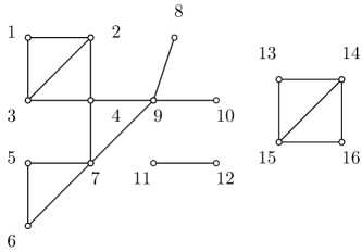
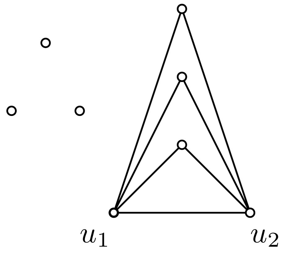
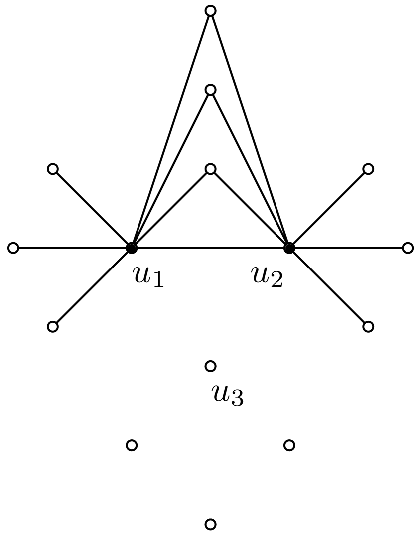
In Fig. 4, we give an example of two graphs $H$ and $H^{\prime}$ satisfying the assumption of Lemma 9. In this example, $|U|=2$, and $|V|=8$. Note that if any of the vertices in $U$ are removed along with all their incident edges, then the resulting graphs are isomorphic. Also, since $H[U]\simeq H^{\prime}[U]$, Lemma 9 implies that ${\rm TV}(P_{{\widetilde{H}}},P_{{\widetilde{H}}^{\prime}})\leq p^{2}(1-(1-p)^{6})$.

(a) The graph $H$.

(b) The graph $H^{\prime}$.

(c) The resulting graph when $u_{1}$ is sampled but not $u_{2}$.

Figure 4: Example where $U=\{u_{1},u_{2}\}$ is an edge. If any of these vertices are not sampled and all incident edges are removed, the resulting graphs are isomorphic.

In the remainder of the section, we apply Theorem 10, Lemma 8, and Lemma 9 to derive lower bounds on the minimax risk for graphs that contain cycles and general chordal graphs, respectively. The main task is to handcraft a pair of graphs $H$ and $H^{\prime}$ that either have matching counts of small subgraphs or for which certain configurations of their vertices induce subgraphs that are isomorphic.

5.3 Lower bound for chordal graphs

Theorem 11 (Chordal graphs).

Let ${\mathcal{G}}(N,d,\omega)$ denote the collection of all chordal graphs on $N$ vertices with maximum degree and clique number at most $d$ and $\omega\geq 2$, respectively. Assume that $p<\frac{1}{2^{\omega}100}$. Then

$$\inf_{\widehat{\mathsf{cc}}}\sup_{G\in{\mathcal{G}}(N,d,\omega)}\mathbb{E}_{G}|\widehat{\mathsf{cc}}-\mathsf{cc}(G)|^{2}=\Theta_{\omega}\left(\left(\frac{N}{p^{\omega}}\vee\frac{Nd}{p^{\omega-1}}\right)\wedge N^{2}\right).$$

Proof.

There are two different constructions we give, according to whether $d\geq 2^{\omega}$ or $d<2^{\omega}$.

Case I: $d\geq 2^{\omega}$.

For every $\omega\geq 2$ and $m\in\mathbb{N}$, we construct a pair of graphs $H$ and $H^{\prime}$, such that

$$v(H)= ~{}v(H^{\prime})=\omega-1+m2^{\omega-2}$$ (32)

$$d_{\max}(H)= ~{}d_{\max}(H^{\prime})=m2^{\omega-3}+\omega-2,\qquad\omega\geq 3$$ (33)

$$d_{\max}(H)= ~{}0,\quad d_{\max}(H^{\prime})=m,\qquad\omega=2$$ (34)

$$\mathsf{cc}(H)= ~{}m+1,\quad\mathsf{cc}(H^{\prime})=1$$ (35)

$$|\mathsf{s}(K_{\omega},H)-\mathsf{s}(K_{\omega},H^{\prime})|= ~{}m$$ (36)

Fix a set of $\omega-1$ vertices $U$ that forms a clique. We first construct $H$. For every subset $S\subset U$ such that $|S|$ is even, let $V_{S}$ be a set of $m$ distinct vertices such that the neighborhood of every $v\in V_{S}$ is given by $\partial v=S$. Let the vertex set $V(H)$ be the union of $U$ and all $V_{S}$ such that $|S|$ is even. In particular, because of the presence of $S=\emptyset$, $H$ always has exactly $m$ isolated vertices (unless $\omega=2$, in which case $H$ consists of $m+1$ isolated vertices). Repeat the same construction for $H^{\prime}$ with $|S|$ being odd. Then both $H$ are $H^{\prime}$ are chordal and have the same number of vertices as in (32), since

$$v(H)=\omega-1+m\sum_{0\leq i\leq\omega-1,~{}i\text{ even}}\binom{\omega-1}{i}=v(H^{\prime})=~{}\omega-1+m\sum_{0\leq i\leq\omega-1,~{}i\text{ odd}}\binom{\omega-1}{i}$$

which follows from the binomial summation formula. Similarly, (33)–(36) can be readily verified.

We also have that

$$\mathsf{s}(K_{i},H) =\binom{\omega-1}{i}+m\sum_{0\leq j\leq\omega-1,~{}j\text{ even}}\binom{\omega-1}{j}\binom{j}{i-1}=$$

$$\mathsf{s}(K_{i},H^{\prime}) =\binom{\omega-1}{i}+m\sum_{0\leq j\leq\omega-1,~{}j\text{ odd}}\binom{\omega-1}{j}\binom{j}{i-1}=\binom{\omega-1}{i}+m\binom{\omega-1}{i-1}2^{\omega-1-i},$$

for $i=1,2,\dots,\omega-1$. This follows from the fact that $\sum_{0\leq j\leq\omega-1}(-1)^{j}\binom{\omega-1}{j}\binom{j}{i-1}=0$ and $\sum_{0\leq j\leq\omega-1}\binom{\omega-1}{j}\binom{j}{i-1}=\binom{\omega-1}{i-1}2^{\omega-i}$.

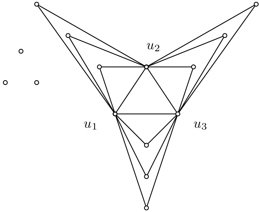
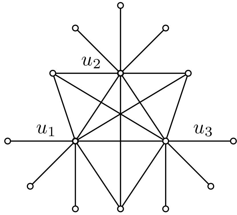
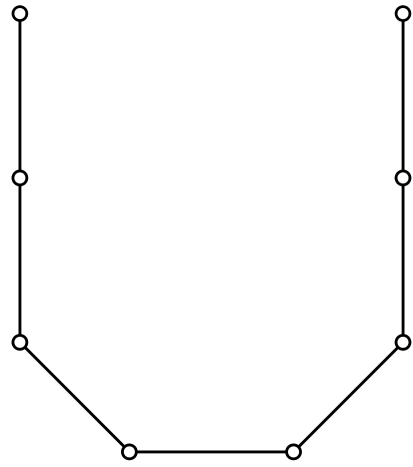
To compute the total variation distance between the sampled graphs, we first assume that $H$ and $H^{\prime}$ are defined on the same set of labelled vertices $V$. The key observation is the following: by construction, $H[U]\simeq H^{\prime}[U]$ (since $U$ induces a clique) and, furthermore, failing to sample any vertex in $U$ results in an isomorphic graph, i.e., $H[V\setminus\{u\}]\simeq H^{\prime}[V\setminus\{u\}]$ for any $u\in U$. Indeed, the structure of the induced subgraph $H[V\setminus\{u\}]$ can be described as follows. First, let $U$ form a clique. Next, for every nonempty subset $S\subset U\setminus\{u\}$, attach a set of $m$ distinct vertices (denoted by $V_{S}$) so that the neighborhood of every $v\in V_{S}$ is given by $\partial v=S$. Finally, add $m+1$ isolated vertices. See Fig. 4 ($\omega=3$) and Fig. 5 ($\omega=4$) for illustrations of this property and the iterative nature of this construction, in the sense that the construction of $H$ (resp. $H^{\prime}$) for $\omega=k+1$ can be obtained from the construction of $H$ (resp. $H^{\prime}$) for $\omega=k$ by adding another vertex $u$ to $U$ such that $\partial u=U$ and then adjoining $m$ distinct vertices to every even (resp. odd) cardinality set $S\subset U$ containing $u$.

Thus by Lemma 9, ${\rm TV}(P_{{\widetilde{H}}},P_{{\widetilde{H}}^{\prime}})\leq p^{|U|}\left(1-(1-p)^{|V|-|U|}\right)=p^{\omega-1}(1-(1-p)^{m2^{\omega-2}})$. According to (33), we choose $m={\left\lfloor{(d-\omega+2)2^{-\omega+3}}\right\rfloor}\geq d2^{-\omega+2}$ if $\omega\geq 3$ and $m=d$ if $\omega=2$. Then we have, ${\rm TV}(P_{{\widetilde{H}}},P_{{\widetilde{H}}^{\prime}})=p^{\omega-1}(1-(1-p)^{d})\leq p^{\omega-1}(pd\wedge 1)$. The condition on $p$ ensures that ${\rm TV}(P_{{\widetilde{H}}},P_{{\widetilde{H}}^{\prime}})\leq p<1/300$. In view of Theorem 10 and (35), we have

$$\inf_{\widehat{\mathsf{cc}}}\sup_{G\in{\mathcal{G}}(N,d,\omega)}\mathbb{E}_{G}|\widehat{\mathsf{cc}}-\mathsf{cc}(G)|^{2}=\Theta_{\omega}\left(\left(\frac{N}{p^{\omega}}\vee\frac{Nd}{p^{\omega-1}}\right)\wedge N^{2}\right),$$

provided $d\geq 2^{\omega}$.

(a) The graph $H$.

(b) The graph $H^{\prime}$.

(c) The resulting graph when $u_{1}$ and $u_{2}$ are sampled but not $u_{3}$.

Figure 5: Example for $\omega=4$ and $m=3$, where $U=\{u_{1},u_{2},u_{3}\}$ form a triangle. If any one or two (as shown in the figure) of these vertices are not sampled and all incident edges are removed, the resulting graphs are isomorphic.

Case II: $d\leq 2^{\omega}$.

In this case, the previous construction is no longer feasible and we must construct another pair of graphs with a smaller maximum degree. To this end, we consider graphs $H$ and $H^{\prime}$ consisting of disjoint cliques of size at most $\omega\geq 2$, such that

$$v(H)=v(H^{\prime})=\omega 2^{\omega-2},\quad d_{\max}(H)=d_{\max}(H^{\prime})=\omega-1,\quad|\mathsf{cc}(H)-\mathsf{cc}(H^{\prime})|=1.$$ (37)

If $\omega$ is odd, we set

$$H= ~{}\tbinom{\omega}{\omega}K_{\omega}+\tbinom{\omega}{\omega-2}K_{\omega-2}+\cdots+\tbinom{\omega}{3}K_{3}+\tbinom{\omega}{1}K_{1}$$ (38)

$$H^{\prime}= ~{}\tbinom{\omega}{\omega-1}K_{\omega-1}+\tbinom{\omega}{\omega-3}K_{\omega-3}+\cdots+\tbinom{\omega}{4}K_{4}+\tbinom{\omega}{2}K_{2}.$$

If $\omega$ is even, we set

$$H= ~{}\tbinom{\omega}{\omega}K_{\omega}+\tbinom{\omega}{\omega-2}K_{\omega-2}+\cdots+\tbinom{\omega}{4}K_{4}+\tbinom{\omega}{2}K_{2}$$ (39)

$$H^{\prime}= ~{}\tbinom{\omega}{\omega-1}K_{\omega-1}+\tbinom{\omega}{\omega-3}K_{\omega-3}+\cdots+\tbinom{\omega}{3}K_{3}+\tbinom{\omega}{1}K_{1}.$$

For example, for $\omega=3$, (38) becomes $H=\leavevmode\hbox to10.51pt{\vbox to9.56pt{\pgfpicture\makeatletter\hbox{\hskip 1.7pt\lower-1.7pt\hbox to0.0pt{\pgfsys@beginscope\pgfsys@invoke{ }\definecolor{pgfstrokecolor}{rgb}{0,0,0}\pgfsys@color@rgb@stroke{0}{0}{0}\pgfsys@invoke{ }\pgfsys@color@rgb@fill{0}{0}{0}\pgfsys@invoke{ }\pgfsys@setlinewidth{0.4pt}\pgfsys@invoke{ }\nullfont\pgfsys@beginscope\pgfsys@invoke{ }\pgfsys@invoke{\lxSVG@closescope }\pgfsys@endscope\hbox to0.0pt{\pgfsys@beginscope\pgfsys@invoke{ }{{}}{{}{{}}{}{{}} {}{}{{}} {}{}{{}} {}{}\pgfsys@moveto{0.0pt}{0.0pt}\pgfsys@lineto{7.11319pt}{0.0pt}\pgfsys@lineto{3.5566pt}{6.16022pt}\pgfsys@closepath\pgfsys@stroke\pgfsys@invoke{ }\hbox{\hbox{\hbox{\hbox{{\pgfsys@beginscope\pgfsys@invoke{ }\definecolor[named]{pgffillcolor}{rgb}{1,1,1}\pgfsys@color@gray@fill{1}\pgfsys@invoke{ }{{}{{{}}}{{}}{}{}{}{}{}{}{}{}{}{\pgfsys@beginscope\pgfsys@invoke{ }\definecolor[named]{pgffillcolor}{rgb}{1,1,1}\pgfsys@color@gray@fill{1}\pgfsys@invoke{ }{}\pgfsys@moveto{1.5pt}{0.0pt}\pgfsys@curveto{1.5pt}{0.82843pt}{0.82843pt}{1.5pt}{0.0pt}{1.5pt}\pgfsys@curveto{-0.82843pt}{1.5pt}{-1.5pt}{0.82843pt}{-1.5pt}{0.0pt}\pgfsys@curveto{-1.5pt}{-0.82843pt}{-0.82843pt}{-1.5pt}{0.0pt}{-1.5pt}\pgfsys@curveto{0.82843pt}{-1.5pt}{1.5pt}{-0.82843pt}{1.5pt}{0.0pt}\pgfsys@closepath\pgfsys@moveto{0.0pt}{0.0pt}\pgfsys@fillstroke\pgfsys@invoke{ } \pgfsys@invoke{\lxSVG@closescope }\pgfsys@endscope}{{{{}}\pgfsys@beginscope\pgfsys@invoke{ }\pgfsys@transformcm{1.0}{0.0}{0.0}{1.0}{0.0pt}{0.0pt}\pgfsys@invoke{ }\hbox{{\definecolor{pgfstrokecolor}{rgb}{0,0,0}\pgfsys@color@rgb@stroke{0}{0}{0}\pgfsys@invoke{ }\pgfsys@color@rgb@fill{0}{0}{0}\pgfsys@invoke{ }\hbox{} }}\pgfsys@invoke{\lxSVG@closescope }\pgfsys@endscope}}} \pgfsys@invoke{\lxSVG@closescope }\pgfsys@endscope}}}\hbox{{\pgfsys@beginscope\pgfsys@invoke{ }\definecolor[named]{pgffillcolor}{rgb}{1,1,1}\pgfsys@color@gray@fill{1}\pgfsys@invoke{ }{{}{{{}}}{{}}{}{}{}{}{}{}{}{}{}{\pgfsys@beginscope\pgfsys@invoke{ }\definecolor[named]{pgffillcolor}{rgb}{1,1,1}\pgfsys@color@gray@fill{1}\pgfsys@invoke{ }{}\pgfsys@moveto{8.61319pt}{0.0pt}\pgfsys@curveto{8.61319pt}{0.82843pt}{7.94162pt}{1.5pt}{7.11319pt}{1.5pt}\pgfsys@curveto{6.28476pt}{1.5pt}{5.61319pt}{0.82843pt}{5.61319pt}{0.0pt}\pgfsys@curveto{5.61319pt}{-0.82843pt}{6.28476pt}{-1.5pt}{7.11319pt}{-1.5pt}\pgfsys@curveto{7.94162pt}{-1.5pt}{8.61319pt}{-0.82843pt}{8.61319pt}{0.0pt}\pgfsys@closepath\pgfsys@moveto{7.11319pt}{0.0pt}\pgfsys@fillstroke\pgfsys@invoke{ } \pgfsys@invoke{\lxSVG@closescope }\pgfsys@endscope}{{{{}}\pgfsys@beginscope\pgfsys@invoke{ }\pgfsys@transformcm{1.0}{0.0}{0.0}{1.0}{7.11319pt}{0.0pt}\pgfsys@invoke{ }\hbox{{\definecolor{pgfstrokecolor}{rgb}{0,0,0}\pgfsys@color@rgb@stroke{0}{0}{0}\pgfsys@invoke{ }\pgfsys@color@rgb@fill{0}{0}{0}\pgfsys@invoke{ }\hbox{} }}\pgfsys@invoke{\lxSVG@closescope }\pgfsys@endscope}}} \pgfsys@invoke{\lxSVG@closescope }\pgfsys@endscope}}}\hbox{{\pgfsys@beginscope\pgfsys@invoke{ }\definecolor[named]{pgffillcolor}{rgb}{1,1,1}\pgfsys@color@gray@fill{1}\pgfsys@invoke{ }{{}{{{}}}{{}}{}{}{}{}{}{}{}{}{}{\pgfsys@beginscope\pgfsys@invoke{ }\definecolor[named]{pgffillcolor}{rgb}{1,1,1}\pgfsys@color@gray@fill{1}\pgfsys@invoke{ }{}\pgfsys@moveto{5.0566pt}{6.16022pt}\pgfsys@curveto{5.0566pt}{6.98865pt}{4.38503pt}{7.66022pt}{3.5566pt}{7.66022pt}\pgfsys@curveto{2.72816pt}{7.66022pt}{2.0566pt}{6.98865pt}{2.0566pt}{6.16022pt}\pgfsys@curveto{2.0566pt}{5.33179pt}{2.72816pt}{4.66022pt}{3.5566pt}{4.66022pt}\pgfsys@curveto{4.38503pt}{4.66022pt}{5.0566pt}{5.33179pt}{5.0566pt}{6.16022pt}\pgfsys@closepath\pgfsys@moveto{3.5566pt}{6.16022pt}\pgfsys@fillstroke\pgfsys@invoke{ } \pgfsys@invoke{\lxSVG@closescope }\pgfsys@endscope}{{{{}}\pgfsys@beginscope\pgfsys@invoke{ }\pgfsys@transformcm{1.0}{0.0}{0.0}{1.0}{3.5566pt}{6.16022pt}\pgfsys@invoke{ }\hbox{{\definecolor{pgfstrokecolor}{rgb}{0,0,0}\pgfsys@color@rgb@stroke{0}{0}{0}\pgfsys@invoke{ }\pgfsys@color@rgb@fill{0}{0}{0}\pgfsys@invoke{ }\hbox{} }}\pgfsys@invoke{\lxSVG@closescope }\pgfsys@endscope}}} \pgfsys@invoke{\lxSVG@closescope }\pgfsys@endscope}}} } \pgfsys@invoke{\lxSVG@closescope }\pgfsys@endscope{{{}}}{}{}\hss}\pgfsys@discardpath\pgfsys@invoke{\lxSVG@closescope }\pgfsys@endscope\hss}}\lxSVG@closescope\endpgfpicture}}+3\times\leavevmode\hbox to3.4pt{\vbox to3.4pt{\pgfpicture\makeatletter\hbox{\hskip 1.7pt\lower-1.7pt\hbox to0.0pt{\pgfsys@beginscope\pgfsys@invoke{ }\definecolor{pgfstrokecolor}{rgb}{0,0,0}\pgfsys@color@rgb@stroke{0}{0}{0}\pgfsys@invoke{ }\pgfsys@color@rgb@fill{0}{0}{0}\pgfsys@invoke{ }\pgfsys@setlinewidth{0.4pt}\pgfsys@invoke{ }\nullfont\pgfsys@beginscope\pgfsys@invoke{ }\pgfsys@invoke{\lxSVG@closescope }\pgfsys@endscope\hbox to0.0pt{\pgfsys@beginscope\pgfsys@invoke{ }{{}}{{}{{}}{}{{}}{}\pgfsys@moveto{0.0pt}{0.0pt}\pgfsys@stroke\pgfsys@invoke{ }\hbox{\hbox{{\pgfsys@beginscope\pgfsys@invoke{ }\definecolor[named]{pgffillcolor}{rgb}{1,1,1}\pgfsys@color@gray@fill{1}\pgfsys@invoke{ }{{}{{{}}}{{}}{}{}{}{}{}{}{}{}{}{\pgfsys@beginscope\pgfsys@invoke{ }\definecolor[named]{pgffillcolor}{rgb}{1,1,1}\pgfsys@color@gray@fill{1}\pgfsys@invoke{ }{}\pgfsys@moveto{1.5pt}{0.0pt}\pgfsys@curveto{1.5pt}{0.82843pt}{0.82843pt}{1.5pt}{0.0pt}{1.5pt}\pgfsys@curveto{-0.82843pt}{1.5pt}{-1.5pt}{0.82843pt}{-1.5pt}{0.0pt}\pgfsys@curveto{-1.5pt}{-0.82843pt}{-0.82843pt}{-1.5pt}{0.0pt}{-1.5pt}\pgfsys@curveto{0.82843pt}{-1.5pt}{1.5pt}{-0.82843pt}{1.5pt}{0.0pt}\pgfsys@closepath\pgfsys@moveto{0.0pt}{0.0pt}\pgfsys@fillstroke\pgfsys@invoke{ } \pgfsys@invoke{\lxSVG@closescope }\pgfsys@endscope}{{{{}}\pgfsys@beginscope\pgfsys@invoke{ }\pgfsys@transformcm{1.0}{0.0}{0.0}{1.0}{0.0pt}{0.0pt}\pgfsys@invoke{ }\hbox{{\definecolor{pgfstrokecolor}{rgb}{0,0,0}\pgfsys@color@rgb@stroke{0}{0}{0}\pgfsys@invoke{ }\pgfsys@color@rgb@fill{0}{0}{0}\pgfsys@invoke{ }\hbox{} }}\pgfsys@invoke{\lxSVG@closescope }\pgfsys@endscope}}} \pgfsys@invoke{\lxSVG@closescope }\pgfsys@endscope}}} } \pgfsys@invoke{\lxSVG@closescope }\pgfsys@endscope{}{}{}\hss}\pgfsys@discardpath\pgfsys@invoke{\lxSVG@closescope }\pgfsys@endscope\hss}}\lxSVG@closescope\endpgfpicture}}$ and $H^{\prime}=3\times\leavevmode\hbox to10.51pt{\vbox to3.4pt{\pgfpicture\makeatletter\hbox{\hskip 1.7pt\lower-1.7pt\hbox to0.0pt{\pgfsys@beginscope\pgfsys@invoke{ }\definecolor{pgfstrokecolor}{rgb}{0,0,0}\pgfsys@color@rgb@stroke{0}{0}{0}\pgfsys@invoke{ }\pgfsys@color@rgb@fill{0}{0}{0}\pgfsys@invoke{ }\pgfsys@setlinewidth{0.4pt}\pgfsys@invoke{ }\nullfont\pgfsys@beginscope\pgfsys@invoke{ }\pgfsys@invoke{\lxSVG@closescope }\pgfsys@endscope\hbox to0.0pt{\pgfsys@beginscope\pgfsys@invoke{ }{{}}{{}{{}}{}{{}} {}{}{{}}{}\pgfsys@moveto{0.0pt}{0.0pt}\pgfsys@lineto{7.11319pt}{0.0pt}\pgfsys@stroke\pgfsys@invoke{ }\hbox{\hbox{\hbox{{\pgfsys@beginscope\pgfsys@invoke{ }\definecolor[named]{pgffillcolor}{rgb}{1,1,1}\pgfsys@color@gray@fill{1}\pgfsys@invoke{ }{{}{{{}}}{{}}{}{}{}{}{}{}{}{}{}{\pgfsys@beginscope\pgfsys@invoke{ }\definecolor[named]{pgffillcolor}{rgb}{1,1,1}\pgfsys@color@gray@fill{1}\pgfsys@invoke{ }{}\pgfsys@moveto{1.5pt}{0.0pt}\pgfsys@curveto{1.5pt}{0.82843pt}{0.82843pt}{1.5pt}{0.0pt}{1.5pt}\pgfsys@curveto{-0.82843pt}{1.5pt}{-1.5pt}{0.82843pt}{-1.5pt}{0.0pt}\pgfsys@curveto{-1.5pt}{-0.82843pt}{-0.82843pt}{-1.5pt}{0.0pt}{-1.5pt}\pgfsys@curveto{0.82843pt}{-1.5pt}{1.5pt}{-0.82843pt}{1.5pt}{0.0pt}\pgfsys@closepath\pgfsys@moveto{0.0pt}{0.0pt}\pgfsys@fillstroke\pgfsys@invoke{ } \pgfsys@invoke{\lxSVG@closescope }\pgfsys@endscope}{{{{}}\pgfsys@beginscope\pgfsys@invoke{ }\pgfsys@transformcm{1.0}{0.0}{0.0}{1.0}{0.0pt}{0.0pt}\pgfsys@invoke{ }\hbox{{\definecolor{pgfstrokecolor}{rgb}{0,0,0}\pgfsys@color@rgb@stroke{0}{0}{0}\pgfsys@invoke{ }\pgfsys@color@rgb@fill{0}{0}{0}\pgfsys@invoke{ }\hbox{} }}\pgfsys@invoke{\lxSVG@closescope }\pgfsys@endscope}}} \pgfsys@invoke{\lxSVG@closescope }\pgfsys@endscope}}}\hbox{{\pgfsys@beginscope\pgfsys@invoke{ }\definecolor[named]{pgffillcolor}{rgb}{1,1,1}\pgfsys@color@gray@fill{1}\pgfsys@invoke{ }{{}{{{}}}{{}}{}{}{}{}{}{}{}{}{}{\pgfsys@beginscope\pgfsys@invoke{ }\definecolor[named]{pgffillcolor}{rgb}{1,1,1}\pgfsys@color@gray@fill{1}\pgfsys@invoke{ }{}\pgfsys@moveto{8.61319pt}{0.0pt}\pgfsys@curveto{8.61319pt}{0.82843pt}{7.94162pt}{1.5pt}{7.11319pt}{1.5pt}\pgfsys@curveto{6.28476pt}{1.5pt}{5.61319pt}{0.82843pt}{5.61319pt}{0.0pt}\pgfsys@curveto{5.61319pt}{-0.82843pt}{6.28476pt}{-1.5pt}{7.11319pt}{-1.5pt}\pgfsys@curveto{7.94162pt}{-1.5pt}{8.61319pt}{-0.82843pt}{8.61319pt}{0.0pt}\pgfsys@closepath\pgfsys@moveto{7.11319pt}{0.0pt}\pgfsys@fillstroke\pgfsys@invoke{ } \pgfsys@invoke{\lxSVG@closescope }\pgfsys@endscope}{{{{}}\pgfsys@beginscope\pgfsys@invoke{ }\pgfsys@transformcm{1.0}{0.0}{0.0}{1.0}{7.11319pt}{0.0pt}\pgfsys@invoke{ }\hbox{{\definecolor{pgfstrokecolor}{rgb}{0,0,0}\pgfsys@color@rgb@stroke{0}{0}{0}\pgfsys@invoke{ }\pgfsys@color@rgb@fill{0}{0}{0}\pgfsys@invoke{ }\hbox{} }}\pgfsys@invoke{\lxSVG@closescope }\pgfsys@endscope}}} \pgfsys@invoke{\lxSVG@closescope }\pgfsys@endscope}}} } \pgfsys@invoke{\lxSVG@closescope }\pgfsys@endscope{}{}{}\hss}\pgfsys@discardpath\pgfsys@invoke{\lxSVG@closescope }\pgfsys@endscope\hss}}\lxSVG@closescope\endpgfpicture}}$ ; for $\omega=4$, (39) becomes $H=\leavevmode\hbox to10.51pt{\vbox to10.51pt{\pgfpicture\makeatletter\hbox{\hskip 1.7pt\lower-1.7pt\hbox to0.0pt{\pgfsys@beginscope\pgfsys@invoke{ }\definecolor{pgfstrokecolor}{rgb}{0,0,0}\pgfsys@color@rgb@stroke{0}{0}{0}\pgfsys@invoke{ }\pgfsys@color@rgb@fill{0}{0}{0}\pgfsys@invoke{ }\pgfsys@setlinewidth{0.4pt}\pgfsys@invoke{ }\nullfont\pgfsys@beginscope\pgfsys@invoke{ }\pgfsys@invoke{\lxSVG@closescope }\pgfsys@endscope\hbox to0.0pt{\pgfsys@beginscope\pgfsys@invoke{ }{{}}{{}{{}}{} {}{}{}\pgfsys@moveto{0.0pt}{0.0pt}\pgfsys@lineto{7.11319pt}{7.11319pt}\pgfsys@stroke\pgfsys@invoke{ } {}{{}}{} {}{}{}\pgfsys@moveto{7.11319pt}{0.0pt}\pgfsys@lineto{0.0pt}{7.11319pt}\pgfsys@stroke\pgfsys@invoke{ } {}{{}}{}{{}} {}{}{{}} {}{}{{}} {}{}{{}} {}{}\pgfsys@moveto{0.0pt}{0.0pt}\pgfsys@lineto{7.11319pt}{0.0pt}\pgfsys@lineto{7.11319pt}{7.11319pt}\pgfsys@lineto{0.0pt}{7.11319pt}\pgfsys@closepath\pgfsys@stroke\pgfsys@invoke{ }\hbox{\hbox{\hbox{\hbox{\hbox{{\pgfsys@beginscope\pgfsys@invoke{ }\definecolor[named]{pgffillcolor}{rgb}{1,1,1}\pgfsys@color@gray@fill{1}\pgfsys@invoke{ }{{}{{{}}}{{}}{}{}{}{}{}{}{}{}{}{\pgfsys@beginscope\pgfsys@invoke{ }\definecolor[named]{pgffillcolor}{rgb}{1,1,1}\pgfsys@color@gray@fill{1}\pgfsys@invoke{ }{}\pgfsys@moveto{1.5pt}{0.0pt}\pgfsys@curveto{1.5pt}{0.82843pt}{0.82843pt}{1.5pt}{0.0pt}{1.5pt}\pgfsys@curveto{-0.82843pt}{1.5pt}{-1.5pt}{0.82843pt}{-1.5pt}{0.0pt}\pgfsys@curveto{-1.5pt}{-0.82843pt}{-0.82843pt}{-1.5pt}{0.0pt}{-1.5pt}\pgfsys@curveto{0.82843pt}{-1.5pt}{1.5pt}{-0.82843pt}{1.5pt}{0.0pt}\pgfsys@closepath\pgfsys@moveto{0.0pt}{0.0pt}\pgfsys@fillstroke\pgfsys@invoke{ } \pgfsys@invoke{\lxSVG@closescope }\pgfsys@endscope}{{{{}}\pgfsys@beginscope\pgfsys@invoke{ }\pgfsys@transformcm{1.0}{0.0}{0.0}{1.0}{0.0pt}{0.0pt}\pgfsys@invoke{ }\hbox{{\definecolor{pgfstrokecolor}{rgb}{0,0,0}\pgfsys@color@rgb@stroke{0}{0}{0}\pgfsys@invoke{ }\pgfsys@color@rgb@fill{0}{0}{0}\pgfsys@invoke{ }\hbox{} }}\pgfsys@invoke{\lxSVG@closescope }\pgfsys@endscope}}} \pgfsys@invoke{\lxSVG@closescope }\pgfsys@endscope}}}\hbox{{\pgfsys@beginscope\pgfsys@invoke{ }\definecolor[named]{pgffillcolor}{rgb}{1,1,1}\pgfsys@color@gray@fill{1}\pgfsys@invoke{ }{{}{{{}}}{{}}{}{}{}{}{}{}{}{}{}{\pgfsys@beginscope\pgfsys@invoke{ }\definecolor[named]{pgffillcolor}{rgb}{1,1,1}\pgfsys@color@gray@fill{1}\pgfsys@invoke{ }{}\pgfsys@moveto{8.61319pt}{0.0pt}\pgfsys@curveto{8.61319pt}{0.82843pt}{7.94162pt}{1.5pt}{7.11319pt}{1.5pt}\pgfsys@curveto{6.28476pt}{1.5pt}{5.61319pt}{0.82843pt}{5.61319pt}{0.0pt}\pgfsys@curveto{5.61319pt}{-0.82843pt}{6.28476pt}{-1.5pt}{7.11319pt}{-1.5pt}\pgfsys@curveto{7.94162pt}{-1.5pt}{8.61319pt}{-0.82843pt}{8.61319pt}{0.0pt}\pgfsys@closepath\pgfsys@moveto{7.11319pt}{0.0pt}\pgfsys@fillstroke\pgfsys@invoke{ } \pgfsys@invoke{\lxSVG@closescope }\pgfsys@endscope}{{{{}}\pgfsys@beginscope\pgfsys@invoke{ }\pgfsys@transformcm{1.0}{0.0}{0.0}{1.0}{7.11319pt}{0.0pt}\pgfsys@invoke{ }\hbox{{\definecolor{pgfstrokecolor}{rgb}{0,0,0}\pgfsys@color@rgb@stroke{0}{0}{0}\pgfsys@invoke{ }\pgfsys@color@rgb@fill{0}{0}{0}\pgfsys@invoke{ }\hbox{} }}\pgfsys@invoke{\lxSVG@closescope }\pgfsys@endscope}}} \pgfsys@invoke{\lxSVG@closescope }\pgfsys@endscope}}}\hbox{{\pgfsys@beginscope\pgfsys@invoke{ }\definecolor[named]{pgffillcolor}{rgb}{1,1,1}\pgfsys@color@gray@fill{1}\pgfsys@invoke{ }{{}{{{}}}{{}}{}{}{}{}{}{}{}{}{}{\pgfsys@beginscope\pgfsys@invoke{ }\definecolor[named]{pgffillcolor}{rgb}{1,1,1}\pgfsys@color@gray@fill{1}\pgfsys@invoke{ }{}\pgfsys@moveto{8.61319pt}{7.11319pt}\pgfsys@curveto{8.61319pt}{7.94162pt}{7.94162pt}{8.61319pt}{7.11319pt}{8.61319pt}\pgfsys@curveto{6.28476pt}{8.61319pt}{5.61319pt}{7.94162pt}{5.61319pt}{7.11319pt}\pgfsys@curveto{5.61319pt}{6.28476pt}{6.28476pt}{5.61319pt}{7.11319pt}{5.61319pt}\pgfsys@curveto{7.94162pt}{5.61319pt}{8.61319pt}{6.28476pt}{8.61319pt}{7.11319pt}\pgfsys@closepath\pgfsys@moveto{7.11319pt}{7.11319pt}\pgfsys@fillstroke\pgfsys@invoke{ } \pgfsys@invoke{\lxSVG@closescope }\pgfsys@endscope}{{{{}}\pgfsys@beginscope\pgfsys@invoke{ }\pgfsys@transformcm{1.0}{0.0}{0.0}{1.0}{7.11319pt}{7.11319pt}\pgfsys@invoke{ }\hbox{{\definecolor{pgfstrokecolor}{rgb}{0,0,0}\pgfsys@color@rgb@stroke{0}{0}{0}\pgfsys@invoke{ }\pgfsys@color@rgb@fill{0}{0}{0}\pgfsys@invoke{ }\hbox{} }}\pgfsys@invoke{\lxSVG@closescope }\pgfsys@endscope}}} \pgfsys@invoke{\lxSVG@closescope }\pgfsys@endscope}}}\hbox{{\pgfsys@beginscope\pgfsys@invoke{ }\definecolor[named]{pgffillcolor}{rgb}{1,1,1}\pgfsys@color@gray@fill{1}\pgfsys@invoke{ }{{}{{{}}}{{}}{}{}{}{}{}{}{}{}{}{\pgfsys@beginscope\pgfsys@invoke{ }\definecolor[named]{pgffillcolor}{rgb}{1,1,1}\pgfsys@color@gray@fill{1}\pgfsys@invoke{ }{}\pgfsys@moveto{1.5pt}{7.11319pt}\pgfsys@curveto{1.5pt}{7.94162pt}{0.82843pt}{8.61319pt}{0.0pt}{8.61319pt}\pgfsys@curveto{-0.82843pt}{8.61319pt}{-1.5pt}{7.94162pt}{-1.5pt}{7.11319pt}\pgfsys@curveto{-1.5pt}{6.28476pt}{-0.82843pt}{5.61319pt}{0.0pt}{5.61319pt}\pgfsys@curveto{0.82843pt}{5.61319pt}{1.5pt}{6.28476pt}{1.5pt}{7.11319pt}\pgfsys@closepath\pgfsys@moveto{0.0pt}{7.11319pt}\pgfsys@fillstroke\pgfsys@invoke{ } \pgfsys@invoke{\lxSVG@closescope }\pgfsys@endscope}{{{{}}\pgfsys@beginscope\pgfsys@invoke{ }\pgfsys@transformcm{1.0}{0.0}{0.0}{1.0}{0.0pt}{7.11319pt}\pgfsys@invoke{ }\hbox{{\definecolor{pgfstrokecolor}{rgb}{0,0,0}\pgfsys@color@rgb@stroke{0}{0}{0}\pgfsys@invoke{ }\pgfsys@color@rgb@fill{0}{0}{0}\pgfsys@invoke{ }\hbox{} }}\pgfsys@invoke{\lxSVG@closescope }\pgfsys@endscope}}} \pgfsys@invoke{\lxSVG@closescope }\pgfsys@endscope}}} } \pgfsys@invoke{\lxSVG@closescope }\pgfsys@endscope{{{}}}{}{}\hss}\pgfsys@discardpath\pgfsys@invoke{\lxSVG@closescope }\pgfsys@endscope\hss}}\lxSVG@closescope\endpgfpicture}}+6\times\leavevmode\hbox to10.51pt{\vbox to3.4pt{\pgfpicture\makeatletter\hbox{\hskip 1.7pt\lower-1.7pt\hbox to0.0pt{\pgfsys@beginscope\pgfsys@invoke{ }\definecolor{pgfstrokecolor}{rgb}{0,0,0}\pgfsys@color@rgb@stroke{0}{0}{0}\pgfsys@invoke{ }\pgfsys@color@rgb@fill{0}{0}{0}\pgfsys@invoke{ }\pgfsys@setlinewidth{0.4pt}\pgfsys@invoke{ }\nullfont\pgfsys@beginscope\pgfsys@invoke{ }\pgfsys@invoke{\lxSVG@closescope }\pgfsys@endscope\hbox to0.0pt{\pgfsys@beginscope\pgfsys@invoke{ }{{}}{{}{{}}{}{{}} {}{}{{}}{}\pgfsys@moveto{0.0pt}{0.0pt}\pgfsys@lineto{7.11319pt}{0.0pt}\pgfsys@stroke\pgfsys@invoke{ }\hbox{\hbox{\hbox{{\pgfsys@beginscope\pgfsys@invoke{ }\definecolor[named]{pgffillcolor}{rgb}{1,1,1}\pgfsys@color@gray@fill{1}\pgfsys@invoke{ }{{}{{{}}}{{}}{}{}{}{}{}{}{}{}{}{\pgfsys@beginscope\pgfsys@invoke{ }\definecolor[named]{pgffillcolor}{rgb}{1,1,1}\pgfsys@color@gray@fill{1}\pgfsys@invoke{ }{}\pgfsys@moveto{1.5pt}{0.0pt}\pgfsys@curveto{1.5pt}{0.82843pt}{0.82843pt}{1.5pt}{0.0pt}{1.5pt}\pgfsys@curveto{-0.82843pt}{1.5pt}{-1.5pt}{0.82843pt}{-1.5pt}{0.0pt}\pgfsys@curveto{-1.5pt}{-0.82843pt}{-0.82843pt}{-1.5pt}{0.0pt}{-1.5pt}\pgfsys@curveto{0.82843pt}{-1.5pt}{1.5pt}{-0.82843pt}{1.5pt}{0.0pt}\pgfsys@closepath\pgfsys@moveto{0.0pt}{0.0pt}\pgfsys@fillstroke\pgfsys@invoke{ } \pgfsys@invoke{\lxSVG@closescope }\pgfsys@endscope}{{{{}}\pgfsys@beginscope\pgfsys@invoke{ }\pgfsys@transformcm{1.0}{0.0}{0.0}{1.0}{0.0pt}{0.0pt}\pgfsys@invoke{ }\hbox{{\definecolor{pgfstrokecolor}{rgb}{0,0,0}\pgfsys@color@rgb@stroke{0}{0}{0}\pgfsys@invoke{ }\pgfsys@color@rgb@fill{0}{0}{0}\pgfsys@invoke{ }\hbox{} }}\pgfsys@invoke{\lxSVG@closescope }\pgfsys@endscope}}} \pgfsys@invoke{\lxSVG@closescope }\pgfsys@endscope}}}\hbox{{\pgfsys@beginscope\pgfsys@invoke{ }\definecolor[named]{pgffillcolor}{rgb}{1,1,1}\pgfsys@color@gray@fill{1}\pgfsys@invoke{ }{{}{{{}}}{{}}{}{}{}{}{}{}{}{}{}{\pgfsys@beginscope\pgfsys@invoke{ }\definecolor[named]{pgffillcolor}{rgb}{1,1,1}\pgfsys@color@gray@fill{1}\pgfsys@invoke{ }{}\pgfsys@moveto{8.61319pt}{0.0pt}\pgfsys@curveto{8.61319pt}{0.82843pt}{7.94162pt}{1.5pt}{7.11319pt}{1.5pt}\pgfsys@curveto{6.28476pt}{1.5pt}{5.61319pt}{0.82843pt}{5.61319pt}{0.0pt}\pgfsys@curveto{5.61319pt}{-0.82843pt}{6.28476pt}{-1.5pt}{7.11319pt}{-1.5pt}\pgfsys@curveto{7.94162pt}{-1.5pt}{8.61319pt}{-0.82843pt}{8.61319pt}{0.0pt}\pgfsys@closepath\pgfsys@moveto{7.11319pt}{0.0pt}\pgfsys@fillstroke\pgfsys@invoke{ } \pgfsys@invoke{\lxSVG@closescope }\pgfsys@endscope}{{{{}}\pgfsys@beginscope\pgfsys@invoke{ }\pgfsys@transformcm{1.0}{0.0}{0.0}{1.0}{7.11319pt}{0.0pt}\pgfsys@invoke{ }\hbox{{\definecolor{pgfstrokecolor}{rgb}{0,0,0}\pgfsys@color@rgb@stroke{0}{0}{0}\pgfsys@invoke{ }\pgfsys@color@rgb@fill{0}{0}{0}\pgfsys@invoke{ }\hbox{} }}\pgfsys@invoke{\lxSVG@closescope }\pgfsys@endscope}}} \pgfsys@invoke{\lxSVG@closescope }\pgfsys@endscope}}} } \pgfsys@invoke{\lxSVG@closescope }\pgfsys@endscope{}{}{}\hss}\pgfsys@discardpath\pgfsys@invoke{\lxSVG@closescope }\pgfsys@endscope\hss}}\lxSVG@closescope\endpgfpicture}}$ and $H^{\prime}=4\times\leavevmode\hbox to10.51pt{\vbox to9.56pt{\pgfpicture\makeatletter\hbox{\hskip 1.7pt\lower-1.7pt\hbox to0.0pt{\pgfsys@beginscope\pgfsys@invoke{ }\definecolor{pgfstrokecolor}{rgb}{0,0,0}\pgfsys@color@rgb@stroke{0}{0}{0}\pgfsys@invoke{ }\pgfsys@color@rgb@fill{0}{0}{0}\pgfsys@invoke{ }\pgfsys@setlinewidth{0.4pt}\pgfsys@invoke{ }\nullfont\pgfsys@beginscope\pgfsys@invoke{ }\pgfsys@invoke{\lxSVG@closescope }\pgfsys@endscope\hbox to0.0pt{\pgfsys@beginscope\pgfsys@invoke{ }{{}}{{}{{}}{}{{}} {}{}{{}} {}{}{{}} {}{}\pgfsys@moveto{0.0pt}{0.0pt}\pgfsys@lineto{7.11319pt}{0.0pt}\pgfsys@lineto{3.5566pt}{6.16022pt}\pgfsys@closepath\pgfsys@stroke\pgfsys@invoke{ }\hbox{\hbox{\hbox{\hbox{{\pgfsys@beginscope\pgfsys@invoke{ }\definecolor[named]{pgffillcolor}{rgb}{1,1,1}\pgfsys@color@gray@fill{1}\pgfsys@invoke{ }{{}{{{}}}{{}}{}{}{}{}{}{}{}{}{}{\pgfsys@beginscope\pgfsys@invoke{ }\definecolor[named]{pgffillcolor}{rgb}{1,1,1}\pgfsys@color@gray@fill{1}\pgfsys@invoke{ }{}\pgfsys@moveto{1.5pt}{0.0pt}\pgfsys@curveto{1.5pt}{0.82843pt}{0.82843pt}{1.5pt}{0.0pt}{1.5pt}\pgfsys@curveto{-0.82843pt}{1.5pt}{-1.5pt}{0.82843pt}{-1.5pt}{0.0pt}\pgfsys@curveto{-1.5pt}{-0.82843pt}{-0.82843pt}{-1.5pt}{0.0pt}{-1.5pt}\pgfsys@curveto{0.82843pt}{-1.5pt}{1.5pt}{-0.82843pt}{1.5pt}{0.0pt}\pgfsys@closepath\pgfsys@moveto{0.0pt}{0.0pt}\pgfsys@fillstroke\pgfsys@invoke{ } \pgfsys@invoke{\lxSVG@closescope }\pgfsys@endscope}{{{{}}\pgfsys@beginscope\pgfsys@invoke{ }\pgfsys@transformcm{1.0}{0.0}{0.0}{1.0}{0.0pt}{0.0pt}\pgfsys@invoke{ }\hbox{{\definecolor{pgfstrokecolor}{rgb}{0,0,0}\pgfsys@color@rgb@stroke{0}{0}{0}\pgfsys@invoke{ }\pgfsys@color@rgb@fill{0}{0}{0}\pgfsys@invoke{ }\hbox{} }}\pgfsys@invoke{\lxSVG@closescope }\pgfsys@endscope}}} \pgfsys@invoke{\lxSVG@closescope }\pgfsys@endscope}}}\hbox{{\pgfsys@beginscope\pgfsys@invoke{ }\definecolor[named]{pgffillcolor}{rgb}{1,1,1}\pgfsys@color@gray@fill{1}\pgfsys@invoke{ }{{}{{{}}}{{}}{}{}{}{}{}{}{}{}{}{\pgfsys@beginscope\pgfsys@invoke{ }\definecolor[named]{pgffillcolor}{rgb}{1,1,1}\pgfsys@color@gray@fill{1}\pgfsys@invoke{ }{}\pgfsys@moveto{8.61319pt}{0.0pt}\pgfsys@curveto{8.61319pt}{0.82843pt}{7.94162pt}{1.5pt}{7.11319pt}{1.5pt}\pgfsys@curveto{6.28476pt}{1.5pt}{5.61319pt}{0.82843pt}{5.61319pt}{0.0pt}\pgfsys@curveto{5.61319pt}{-0.82843pt}{6.28476pt}{-1.5pt}{7.11319pt}{-1.5pt}\pgfsys@curveto{7.94162pt}{-1.5pt}{8.61319pt}{-0.82843pt}{8.61319pt}{0.0pt}\pgfsys@closepath\pgfsys@moveto{7.11319pt}{0.0pt}\pgfsys@fillstroke\pgfsys@invoke{ } \pgfsys@invoke{\lxSVG@closescope }\pgfsys@endscope}{{{{}}\pgfsys@beginscope\pgfsys@invoke{ }\pgfsys@transformcm{1.0}{0.0}{0.0}{1.0}{7.11319pt}{0.0pt}\pgfsys@invoke{ }\hbox{{\definecolor{pgfstrokecolor}{rgb}{0,0,0}\pgfsys@color@rgb@stroke{0}{0}{0}\pgfsys@invoke{ }\pgfsys@color@rgb@fill{0}{0}{0}\pgfsys@invoke{ }\hbox{} }}\pgfsys@invoke{\lxSVG@closescope }\pgfsys@endscope}}} \pgfsys@invoke{\lxSVG@closescope }\pgfsys@endscope}}}\hbox{{\pgfsys@beginscope\pgfsys@invoke{ }\definecolor[named]{pgffillcolor}{rgb}{1,1,1}\pgfsys@color@gray@fill{1}\pgfsys@invoke{ }{{}{{{}}}{{}}{}{}{}{}{}{}{}{}{}{\pgfsys@beginscope\pgfsys@invoke{ }\definecolor[named]{pgffillcolor}{rgb}{1,1,1}\pgfsys@color@gray@fill{1}\pgfsys@invoke{ }{}\pgfsys@moveto{5.0566pt}{6.16022pt}\pgfsys@curveto{5.0566pt}{6.98865pt}{4.38503pt}{7.66022pt}{3.5566pt}{7.66022pt}\pgfsys@curveto{2.72816pt}{7.66022pt}{2.0566pt}{6.98865pt}{2.0566pt}{6.16022pt}\pgfsys@curveto{2.0566pt}{5.33179pt}{2.72816pt}{4.66022pt}{3.5566pt}{4.66022pt}\pgfsys@curveto{4.38503pt}{4.66022pt}{5.0566pt}{5.33179pt}{5.0566pt}{6.16022pt}\pgfsys@closepath\pgfsys@moveto{3.5566pt}{6.16022pt}\pgfsys@fillstroke\pgfsys@invoke{ } \pgfsys@invoke{\lxSVG@closescope }\pgfsys@endscope}{{{{}}\pgfsys@beginscope\pgfsys@invoke{ }\pgfsys@transformcm{1.0}{0.0}{0.0}{1.0}{3.5566pt}{6.16022pt}\pgfsys@invoke{ }\hbox{{\definecolor{pgfstrokecolor}{rgb}{0,0,0}\pgfsys@color@rgb@stroke{0}{0}{0}\pgfsys@invoke{ }\pgfsys@color@rgb@fill{0}{0}{0}\pgfsys@invoke{ }\hbox{} }}\pgfsys@invoke{\lxSVG@closescope }\pgfsys@endscope}}} \pgfsys@invoke{\lxSVG@closescope }\pgfsys@endscope}}} } \pgfsys@invoke{\lxSVG@closescope }\pgfsys@endscope{{{}}}{}{}\hss}\pgfsys@discardpath\pgfsys@invoke{\lxSVG@closescope }\pgfsys@endscope\hss}}\lxSVG@closescope\endpgfpicture}}+4\times\leavevmode\hbox to3.4pt{\vbox to3.4pt{\pgfpicture\makeatletter\hbox{\hskip 1.7pt\lower-1.7pt\hbox to0.0pt{\pgfsys@beginscope\pgfsys@invoke{ }\definecolor{pgfstrokecolor}{rgb}{0,0,0}\pgfsys@color@rgb@stroke{0}{0}{0}\pgfsys@invoke{ }\pgfsys@color@rgb@fill{0}{0}{0}\pgfsys@invoke{ }\pgfsys@setlinewidth{0.4pt}\pgfsys@invoke{ }\nullfont\pgfsys@beginscope\pgfsys@invoke{ }\pgfsys@invoke{\lxSVG@closescope }\pgfsys@endscope\hbox to0.0pt{\pgfsys@beginscope\pgfsys@invoke{ }{{}}{{}{{}}{}{{}}{}\pgfsys@moveto{0.0pt}{0.0pt}\pgfsys@stroke\pgfsys@invoke{ }\hbox{\hbox{{\pgfsys@beginscope\pgfsys@invoke{ }\definecolor[named]{pgffillcolor}{rgb}{1,1,1}\pgfsys@color@gray@fill{1}\pgfsys@invoke{ }{{}{{{}}}{{}}{}{}{}{}{}{}{}{}{}{\pgfsys@beginscope\pgfsys@invoke{ }\definecolor[named]{pgffillcolor}{rgb}{1,1,1}\pgfsys@color@gray@fill{1}\pgfsys@invoke{ }{}\pgfsys@moveto{1.5pt}{0.0pt}\pgfsys@curveto{1.5pt}{0.82843pt}{0.82843pt}{1.5pt}{0.0pt}{1.5pt}\pgfsys@curveto{-0.82843pt}{1.5pt}{-1.5pt}{0.82843pt}{-1.5pt}{0.0pt}\pgfsys@curveto{-1.5pt}{-0.82843pt}{-0.82843pt}{-1.5pt}{0.0pt}{-1.5pt}\pgfsys@curveto{0.82843pt}{-1.5pt}{1.5pt}{-0.82843pt}{1.5pt}{0.0pt}\pgfsys@closepath\pgfsys@moveto{0.0pt}{0.0pt}\pgfsys@fillstroke\pgfsys@invoke{ } \pgfsys@invoke{\lxSVG@closescope }\pgfsys@endscope}{{{{}}\pgfsys@beginscope\pgfsys@invoke{ }\pgfsys@transformcm{1.0}{0.0}{0.0}{1.0}{0.0pt}{0.0pt}\pgfsys@invoke{ }\hbox{{\definecolor{pgfstrokecolor}{rgb}{0,0,0}\pgfsys@color@rgb@stroke{0}{0}{0}\pgfsys@invoke{ }\pgfsys@color@rgb@fill{0}{0}{0}\pgfsys@invoke{ }\hbox{} }}\pgfsys@invoke{\lxSVG@closescope }\pgfsys@endscope}}} \pgfsys@invoke{\lxSVG@closescope }\pgfsys@endscope}}} } \pgfsys@invoke{\lxSVG@closescope }\pgfsys@endscope{}{}{}\hss}\pgfsys@discardpath\pgfsys@invoke{\lxSVG@closescope }\pgfsys@endscope\hss}}\lxSVG@closescope\endpgfpicture}}$.

Next we verify that $H$ and $H^{\prime}$ have matching subgraph counts. Indeed, for $i=1,2,\dots,\omega-1$, $\mathsf{s}(K_{i},H)-\mathsf{s}(K_{i},H^{\prime})=\sum_{k=i}^{\omega}(-1)^{k}\tbinom{\omega}{k}\tbinom{k}{i}=0$ and $\mathsf{s}(K_{i},H)=\mathsf{s}(K_{i},H^{\prime})=\frac{1}{2}\sum_{k=i}^{\omega}\tbinom{\omega}{k}\tbinom{k}{i}=2^{\omega-1-i}\tbinom{\omega}{i}$. Hence $H$ and $H^{\prime}$ contain matching number of cliques up to size $\omega-1$. Note that the only connected induced subgraphs of $H$ and $H^{\prime}$ with at most $\omega-1$ vertices are cliques. Consequently, by (30), ${\rm TV}(P_{{\widetilde{H}}},P_{{\widetilde{H}}^{\prime}})\leq\binom{\omega 2^{\omega-2}}{\omega}p^{\omega}$ and together with Theorem 10 and (37), we have

$$\inf_{\widehat{\mathsf{cc}}}\sup_{G\in{\mathcal{G}}(N,d,\omega)}\mathbb{E}_{G}|\widehat{\mathsf{cc}}-\mathsf{cc}(G)|^{2}\geq\Omega_{\omega}\left(\frac{N}{p^{\omega}}\wedge N^{2}\right)=\Theta_{\omega}\left(\left(\frac{N}{p^{\omega}}\vee\frac{Nd}{p^{\omega-1}}\right)\wedge N^{2}\right),$$

where the last inequality follows from the current assumption that $d\leq 2^{\omega}$. The condition on $p$ ensures that ${\rm TV}(P_{{\widetilde{H}}},P_{{\widetilde{H}}^{\prime}})\leq p2^{\omega-2}<1/300$. ∎

Appendix A Additional proofs

In this appendix, we give the proofs of Lemma 1, Lemma 4, Lemma 5, Lemma 6, Theorem 7, Theorem 8, Theorem 9, Theorem 10, Lemma 7, and Lemma 8. We also state the concentration inequality from Lemma 10 that was used in the proof of Theorem 6.

Proof of Lemma 1.

By [56, Theorem 5.3.26], the chromatic polynomial of $G$ is

$$\chi(G;x)=(x-{\mathsf{c}}_{1})\cdots(x-{\mathsf{c}}_{N})=(x-{\mathsf{c}}^{\prime}_{1})\cdots(x-{\mathsf{c}}^{\prime}_{N}).$$

The conclusion follows from the uniqueness of the chromatic polynomial (and its roots). ∎

Proof of Lemma 4.

Note that $\{v_{1},\dots,v_{N}\}$ is also a PEO of ${\widetilde{G}}$ and hence by Lemma 1, there is a bijection between $\{\widetilde{{\mathsf{c}}}_{j}:j\in[m]\}$ and $\{\widehat{{\mathsf{c}}}_{j}:j\in[N]\}$. Therefore

$$\widehat{{\mathsf{g}}}=\sum_{j=1}^{m}g(\widetilde{{\mathsf{c}}}_{j})=\sum_{j=1}^{N}b_{j}g(\widehat{{\mathsf{c}}}_{j}).\qed$$

Proof of Lemma 5.

Note that $N_{S}+N_{T}=N_{S\setminus T}+N_{T\setminus S}+2N_{S\cap T}$, where $N_{S\setminus T}$, $N_{T\setminus S}$, and $N_{S\cap T}$ are independent binomially distributed random variables. By independence, we have

$$\mathbb{E}[f(N_{S})f(N_{T})] =\mathbb{E}\left[\left(-\frac{q}{p}\right)^{N_{S}+N_{T}}\right]=\mathbb{E}\left[\left(-\frac{q}{p}\right)^{N_{S\setminus T}+N_{T\setminus S}+2N_{S\cap T}}\right]$$

$$=\mathbb{E}\left[\left(-\frac{q}{p}\right)^{N_{S\setminus T}}\right]\mathbb{E}\left[\left(-\frac{q}{p}\right)^{N_{T\setminus S}}\right]\mathbb{E}\left[\left(-\frac{q}{p}\right)^{2N_{S\cap T}}\right].$$

Finally, note that if $S\neq T$, then at least one of $\mathbb{E}[(-\frac{q}{p})^{N_{S\setminus T}}]$ or $\mathbb{E}[(-\frac{q}{p})^{N_{T\setminus S}}]$ is zero. If $S=T$, we have

$$\mathbb{E}[f(N_{S})^{2}]=\mathbb{E}\left[\left(-\frac{q}{p}\right)^{2N_{S}}\right]=\left(\frac{q}{p}\right)^{|{S}|}.$$

∎

Proof of Lemma 6.

Let ${\mathsf{c}}_{j}=|C_{j}|$. To prove (15), we will show that for any fixed $j$,

$$|\{i\in[N]:i\neq j,\;C_{j}=C_{i}\neq\emptyset\}|\leq d-{\mathsf{c}}_{j}\leq d-1.$$

By definition of the PEO, $|N_{G}(v)|\geq{\mathsf{c}}_{j}$ for all $v\in C_{j}$. For any $i\in[N]$ such that $C_{j}=C_{i}\neq\emptyset$, $v_{i}\in N_{G}(v)$ for all $v\in C_{j}$. Also, the fact that $C_{j}=C_{i}\neq\emptyset$ makes it impossible for $v_{i}\in C_{j}$. This shows that

$${\mathsf{c}}_{j}+|\{i\in[N]:i\neq j,\;C_{j}=C_{i}\neq\emptyset\}|\leq|N_{G}(v)|\leq d,$$

and hence the desired (15).

Next, we show (17). Let ${\mathsf{a}}_{j}=|A_{j}|$. We will prove that for any fixed $j$,

$$|\{i\in[N]:i\neq j,\;A_{i}\cap A_{j}\neq\emptyset\}|\leq d{\mathsf{a}}_{j}-({\mathsf{a}}_{j}-1)^{2}.$$ (40)

This fact immediately implies (44) by noting that ${\mathsf{a}}_{j}\leq\omega$. To this end, note that

$$|\{i\in[N]:i\neq j,\;A_{i}\cap A_{j}\neq\emptyset\}| =|\{i\in[N]:i\neq j,\;v_{i}\notin A_{j},\;A_{i}\cap A_{j}\neq\emptyset\}|+$$

$$\qquad|\{i\in[N]:i\neq j,\;v_{i}\in A_{j}\}|,$$

where the second term is obviously at most ${\mathsf{a}}_{j}-1$. Next we prove that the first term is at most $(d+1-{\mathsf{a}}_{j}){\mathsf{a}}_{j}$, which, in view of $(d+1-{\mathsf{a}}_{j}){\mathsf{a}}_{j}+({\mathsf{a}}_{j}-1)=d{\mathsf{a}}_{j}-({\mathsf{a}}_{j}-1)^{2}$, implies the desired (40). Suppose, for the sake of contradiction, that

$$|\{i\in[N]:i\neq j,\;v_{i}\notin A_{j},\;A_{i}\cap A_{j}\neq\emptyset\}|\geq(d+1-{\mathsf{a}}_{j}){\mathsf{a}}_{j}+1$$

Then at least $(d+1-{\mathsf{a}}_{j}){\mathsf{a}}_{j}+1$ of the $A_{i}$ have nonempty intersection with $A_{j}$, meaning that at least $(d+1-{\mathsf{a}}_{j}){\mathsf{a}}_{j}+1$ vertices outside $A_{j}$ are incident to vertices in $A_{j}$. By the pigeonhole principle, there is at least one vertex $u\in A_{j}$ which is incident to $d+2-{\mathsf{a}}_{j}$ of those vertices outside $A_{j}$. Moreover, the vertices in $A_{j}$ form a clique of size ${\mathsf{a}}_{j}$ in $G$ by definition of the PEO. This implies that $|N_{G}(u)|\geq({\mathsf{a}}_{j}-1)+(d-{\mathsf{a}}_{j}+2)=d+1$, contradicting the maximum degree assumption and completing the proof. ∎

To prove the high-probability bound (12), we used a concentration inequality for the sum of dependent random variables due to Janson [34]. This result, stated next, can be distilled from [34, Theorem 2.3]. The two-sided version of the concentration inequality therein also holds; see the paragraph before [34, Equation (2.3)].

Lemma 10.

Let $X=\sum_{j\in[N]}Y_{j}$, where $|Y_{j}-\mathbb{E}\left[Y_{j}\right]|\leq b$ almost surely. Let $S=\sum_{j\in[N]}\mathsf{Var}[Y_{j}]$. Let $\Gamma=([N],E(\Gamma))$ be a dependency graph for $\{Y_{j}\}_{j\in[N]}$ in the sense that if $A\subset[N]$, and $i\in[N]\backslash A$ does not belong to the neighborhood of any vertex in $A$, then $Y_{i}$ is independent of $\{Y_{j}\}_{j\in A}$. Furthermore, suppose $\Gamma$ has maximum degree $d_{\max}$. Then, for all $t\geq 0$,

$$\mathbb{P}\left[|X-\mathbb{E}\left[X\right]|\geq t\right]\leq 2\exp\left\{-\frac{8t^{2}}{25(d_{\max}+1)(S+bt/3)}\right\}.$$

Proof of Theorem 7.

Let $\{v_{1},\dots,v_{N}\}$ be a PEO of the parent graph $G$ and let $\{\widetilde{v}_{1},\dots,\widetilde{v}_{m}\}$, $m=|S|$, be a PEO of ${\widetilde{G}}$ and $\widetilde{{\mathsf{c}}}_{j}=|N_{{\widetilde{G}}}(\widetilde{v}_{j})\cap\{\widetilde{v}_{1},\dots,\widetilde{v}_{j-1}\}|$. Let $\widehat{{\mathsf{c}}}_{j}=|N_{{\widetilde{G}}}(v_{j})\cap\{v_{1},\dots,v_{j-1}\}|$ and ${\mathsf{c}}_{j}=|N_{G}(v_{j})\cap\{v_{1},\dots,v_{j-1}\}|$. By Lemma 4, we can rewrite $\widehat{\mathsf{cc}}_{L}$ as

$$\widehat{\mathsf{cc}}_{L} =\frac{1}{p}\sum_{j\geq 1}b_{j}\left(-\frac{q}{p}\right)^{\widehat{{\mathsf{c}}}_{j}}\mathbb{P}\left[L\geq\widehat{{\mathsf{c}}}_{j}\right],$$

where $\widehat{{\mathsf{c}}}_{j}\sim\mathrm{Bin}({\mathsf{c}}_{j},p)$ conditioned on $\{b_{j}=1\}$.

We compute the bias and variance of $\widehat{\mathsf{cc}}_{L}$ and then optimize over $\lambda$. First,

$$\mathbb{E}[\mathsf{cc}(G)-\widehat{\mathsf{cc}}_{L}] =\frac{1}{p}\sum_{j=1}^{N}\mathbb{E}[b_{j}\left(-\frac{q}{p}\right)^{\widehat{{\mathsf{c}}}_{j}}\mathbb{P}\left[L<\widehat{{\mathsf{c}}}_{j}\right]]=\sum_{j=1}^{N}\sum_{i=0}^{{\mathsf{c}}_{j}}\binom{{\mathsf{c}}_{j}}{i}p^{i}q^{{\mathsf{c}}_{j}-i}\left(-\frac{q}{p}\right)^{i}\mathbb{P}\left[L<i\right]$$

$$=\sum_{j=1}^{N}q^{{\mathsf{c}}_{j}}\sum_{i=0}^{{\mathsf{c}}_{j}}\binom{{\mathsf{c}}_{j}}{i}(-1)^{i}\mathbb{P}\left[L<i\right]=\sum_{j=1}^{N}q^{{\mathsf{c}}_{j}}\sum_{i=0}^{{\mathsf{c}}_{j}}\binom{{\mathsf{c}}_{j}}{i}(-1)^{i}\sum_{\ell=0}^{i-1}\mathbb{P}\left[L=\ell\right]$$

$$=\sum_{j=1}^{N}q^{{\mathsf{c}}_{j}}\sum_{\ell=0}^{{\mathsf{c}}_{j}-1}\mathbb{P}\left[L=\ell\right]\sum_{i=\ell+1}^{{\mathsf{c}}_{j}}\binom{{\mathsf{c}}_{j}}{i}(-1)^{i}$$

$$\overset{\rm(a)}{=}\sum_{j=1}^{N}q^{{\mathsf{c}}_{j}}\mathbb{E}_{L}\left[\binom{{\mathsf{c}}_{j}-1}{L}(-1)^{L+1}\right]$$

$$\overset{\rm(b)}{=}-e^{-\lambda}\sum_{j=1}^{N}q^{{\mathsf{c}}_{j}}L_{{\mathsf{c}}_{j}-1}(\lambda),$$

where (a) follows from the fact that $\sum_{i=\ell+1}^{k}\binom{k}{i}(-1)^{i}=\binom{k-1}{\ell}(-1)^{\ell+1}$, and (b) follows from

$$\mathbb{E}_{L}\left[\binom{k-1}{L}(-1)^{L+1}\right]=e^{-\lambda}L_{k-1}(\lambda),$$ (41)

where $L_{m}$ is the Laguerre polynomial of degree $m$, which satisfies $|L_{m}(x)|\leq e^{x/2}$ for all $m\geq 0$ and $x\geq 0$ [1]. Thus

$$|\mathbb{E}[\widehat{\mathsf{cc}}_{L}-\widehat{\mathsf{cc}}]|\leq Ne^{-\lambda/2}.$$ (42)

To bound the variance, write $\widehat{\mathsf{cc}}_{L}=\frac{1}{p}\sum_{j=1}^{N}W_{j}$, where $W_{j}=b_{j}(-\frac{q}{p})^{\widehat{{\mathsf{c}}}_{j}}\mathbb{P}\left[L\geq\widehat{{\mathsf{c}}}_{j}\right]$. Thus

$$\mathsf{Var}[\widehat{\mathsf{cc}}_{L}]=\frac{1}{p^{2}}\sum_{j\in[N]}\mathsf{Var}[W_{j}]+\frac{1}{p^{2}}\sum_{i\neq j}\mathsf{Cov}[W_{i},W_{j}]$$ (43)

Note that $W_{j}$ is a function of $\{b_{\ell}:v_{\ell}\in A_{j},\ell\in[N]\}$, where $A_{j}$ is defined in (16). Using Lemma 6, we have

$$|\{(i,j)\in[N]^{2}:i\neq j,\;A_{i}\cap A_{j}\neq\emptyset\}|\leq Nd\omega.$$ (44)

Thus the number of cross terms in (43) is at most $Nd\omega$ thanks to (44). Thus,

$$\mathsf{Var}[\widehat{\mathsf{cc}}_{L}]\leq\frac{N(1+d\omega)}{p^{2}}\max_{1\leq j\leq N}\mathsf{Var}[W_{j}].$$ (45)

Finally, note that if $p<1/2$, then

$$\mathsf{Var}[W_{j}]\leq p\left(\sup_{k\geq 0}\left\{\left(\frac{q}{p}\right)^{k}\mathbb{P}\left[L\geq k\right]\right\}\right)^{2}\leq p\left(\mathbb{E}_{L}\left[\left(\frac{q}{p}\right)^{L}\right]\right)^{2}=p\exp\left\{2\lambda\left(\frac{q}{p}-1\right)\right\}.$$ (46)

Combining (42), (45), and (46), we have

$$\mathbb{E}_{G}|\widehat{\mathsf{cc}}_{L}-\mathsf{cc}(G)|^{2}\leq N^{2}e^{-\lambda}+\frac{N(1+d\omega)}{p}\exp\left\{2\lambda\left(\frac{q}{p}-1\right)\right\}.$$

The choice of $\lambda$ yields the desired bound. ∎

Proof of Theorem 8.

The estimator (9) can also be written as $\widehat{\mathsf{cc}}=\sum_{k=1}^{\mathsf{cc}(G)}[1-(-\frac{q}{p})^{\widetilde{N}_{k}}]$, where $\widetilde{N}_{k}$ is the number of sampled vertices from the $k{{}^{\rm th}}$ component. Then $\widetilde{N}_{k}{\stackrel{{\scriptstyle\text{ind.}}}{{\sim}}}\mathrm{Bin}(N_{k},p)$. Thus,

$$\mathsf{Var}[\widehat{\mathsf{cc}}]=\sum_{k=1}^{\mathsf{cc}(G)}\left(\frac{q}{p}\right)^{N_{k}}=\sum_{r=1}^{N}\left(\frac{q}{p}\right)^{r}\mathsf{cc}_{r}.$$

The upper bound follows from the fact that $\mathsf{cc}_{r}=0$ for all $r>\omega$ and $\sum_{r=1}^{N}\mathsf{cc}_{r}=\mathsf{cc}(G)\leq N$. ∎

Proof of Theorem 9.

The bias of this estimator is seen to be

$$\mathbb{E}\left[\mathsf{cc}(G)-\widetilde{\mathsf{cc}}_{L}\right]=\sum_{k=1}^{\mathsf{cc}(G)}\mathbb{E}\left[\mathbb{P}\left[L<\widetilde{N}_{k}\right]\left(-\frac{q}{p}\right)^{\widetilde{N}_{k}}\right].$$

Note that

$$\mathbb{E}\left[\mathbb{P}\left[L<\widetilde{N}_{k}\right]\left(-\frac{q}{p}\right)^{\widetilde{N}_{k}}\right] =\sum_{r=1}^{N}\mathbb{P}\left[L<r\right]\left(-\frac{q}{p}\right)^{r}\mathbb{P}\left[\widetilde{N}_{k}=r\right]$$

$$=\sum_{i=0}^{N-1}\mathbb{P}\left[L=i\right]\sum_{r=i+1}^{N}\left(-\frac{q}{p}\right)^{r}\mathbb{P}\left[\widetilde{N}_{k}=r\right].$$

Since $\widetilde{N}_{k}\sim\text{Bin}(N_{k},p)$, it follows that

$$\sum_{r=i+1}^{N}\left(-\frac{q}{p}\right)^{r}\mathbb{P}\left[\widetilde{N}_{k}=r\right]=q^{N_{k}}\sum_{r=i+1}^{N}\binom{N_{k}}{r}(-1)^{r}=q^{N_{k}}(-1)^{i+1}\binom{N_{k}-1}{i}.$$

Putting these facts together, we have

$$\mathbb{E}\left[\mathsf{cc}(G)-\widetilde{\mathsf{cc}}_{L}\right]=-\sum_{k=1}^{\mathsf{cc}(G)}q^{N_{k}}P_{N_{k}-1}(\lambda)=\sum_{k=1}^{\mathsf{cc}(G)}q^{N_{k}}\mathbb{E}_{L}\left[\binom{N_{k}-1}{L}(-1)^{L+1}\right],$$

Analogous to (41), we have $\left|\mathbb{E}_{L}\left[\binom{N_{k}-1}{L}(-1)^{L+1}\right]\right|\leq e^{-\lambda/2}$, and hence by the Cauchy-Schwarz inequality,

$$|\mathbb{E}\left[\mathsf{cc}(G)-\widetilde{\mathsf{cc}}_{L}\right]|\leq e^{-\lambda/2}\sqrt{N\sum_{k=1}^{\mathsf{cc}(G)}q^{N_{k}}}.$$ (47)

For the variance of $\widetilde{\mathsf{cc}}_{L}$, note that $\widetilde{\mathsf{cc}}_{L}=\sum_{k=1}^{\mathsf{cc}(G)}W_{k}$, where $W_{k}\triangleq 1-\mathbb{P}\left[L\geq\widetilde{N}_{k}\right]\left(-\frac{q}{p}\right)^{\widetilde{N}_{k}}$. The $W_{k}$ are independent random variables and hence

$$\mathsf{Var}[\widetilde{\mathsf{cc}}_{L}]=\sum_{k=1}^{\mathsf{cc}(G)}\mathsf{Var}[W_{k}]\leq\sum_{k=1}^{\mathsf{cc}(G)}\mathbb{E}W^{2}_{k}.$$

Also,

$$W^{2}_{k}\leq\max_{1\leq r\leq N}\left\{1-\mathbb{P}\left[L\geq r\right]\left(-\frac{q}{p}\right)^{r}\right\}^{2}\mathbbm{1}\{\widetilde{N}_{k}\geq 1\}.$$

This means that

$$\mathsf{Var}[\widetilde{\mathsf{cc}}_{L}]\leq\max_{1\leq r\leq N}\left\{1-\mathbb{P}\left[L\geq r\right]\left(-\frac{q}{p}\right)^{r}\right\}^{2}\sum_{k=1}^{\mathsf{cc}(G)}(1-q^{N_{k}}).$$

Since $p<1/2$, we have

$$\mathbb{P}\left[L\geq r\right]\left(\frac{q}{p}\right)^{r} =\sum_{i=r}^{\infty}\mathbb{P}\left[L=i\right]\left(\frac{q}{p}\right)^{r}\leq\sum_{i=r}^{\infty}\mathbb{P}\left[L=i\right]\left(\frac{q}{p}\right)^{i}$$

$$\leq\sum_{i=0}^{\infty}\mathbb{P}\left[L=i\right]\left(\frac{q}{p}\right)^{i}=\mathbb{E}_{L}\left(\frac{q}{p}\right)^{L}=e^{\lambda(\frac{q}{p}-1)}.$$

Thus, it follows that

$$\mathsf{Var}[\widetilde{\mathsf{cc}}_{L}]\leq 4e^{2\lambda(\frac{q}{p}-1)}\sum_{k=1}^{\mathsf{cc}(G)}(1-q^{N_{k}}).$$ (48)

Combining (47) and (48) yields

$$\mathbb{E}|\widetilde{\mathsf{cc}}_{L}-\mathsf{cc}(G)|^{2}\leq 4e^{2\lambda(\frac{q}{p}-1)}\sum_{k=1}^{\mathsf{cc}(G)}(1-q^{N_{k}})+Ne^{-\lambda}\sum_{k=1}^{\mathsf{cc}(G)}q^{N_{k}}\leq\mathsf{cc}(G)\max\left\{4e^{2\lambda(\frac{q}{p}-1)},Ne^{-\lambda}\right\}.$$

Choosing $\lambda=\frac{p}{2-3p}\log(N/4)$ leads to $4e^{2\lambda(\frac{q}{p}-1)}=Ne^{-\lambda}$ and completes the proof. ∎

Proof of Theorem 10.

Fix $\alpha\in(0,1)$. Let $M=N/m$ and $G=G_{1}+G_{2}+\cdots+G_{M}$, where $G_{i}\simeq H$ or $H^{\prime}$ with probability $\alpha$ and $1-\alpha$, respectively. Let $\mathbb{P}_{\alpha}$ denote the law of $G$ and $\mathbb{E}_{\alpha}$ the corresponding expectation. Assume without loss of generality that $f(H)>f(H^{\prime})$. Note that $\mathbb{E}_{\alpha}f(G)=M[\alpha f(H)+(1-\alpha)f(H^{\prime})]$.

Let ${\widetilde{G}}_{i}$ be the sample version of $G_{i}$. Then ${\widetilde{G}}={\widetilde{G}}_{1}+\dots+{\widetilde{G}}_{M}$. For each subgraph $h$, by (2), we have

$$\mathbb{P}\left[{\widetilde{G}}_{i}\simeq h\mid G_{i}\simeq H\right]=\mathsf{s}(h,H)p^{{\mathsf{v}}(h)}(1-p)^{m-{\mathsf{v}}(h)},$$

and

$$\mathbb{P}\left[{\widetilde{G}}_{i}\simeq h\mid G_{i}\simeq H^{\prime}\right]=\mathsf{s}(h,H^{\prime})p^{{\mathsf{v}}(h)}(1-p)^{m-{\mathsf{v}}(h)}.$$

Let $P\triangleq P_{{\widetilde{H}}}=\mathcal{L}({\widetilde{G}}_{i}\mid G_{i}\simeq H)$ and $P^{\prime}\triangleq P_{{\widetilde{H}}^{\prime}}=\mathcal{L}({\widetilde{G}}_{i}\mid G_{i}\simeq H^{\prime})$. Then the law of each ${\widetilde{G}}_{i}$ is simply a mixture $P_{\alpha}\triangleq\mathcal{L}({\widetilde{G}}_{i})=\alpha P+(1-\alpha)P^{\prime}$. Furthermore, $({\widetilde{G}}_{1},{\widetilde{G}}_{2},\dots,{\widetilde{G}}_{M})^{\prime}\sim P^{\otimes M}_{\alpha}$.

To lower bound the minimax risk of estimating the functional $f(G)$, we apply the method of two fuzzy hypotheses [55, Theorem 2.15(i)]. To this end, consider a pair of priors, that is, the distribution of $G$ with $\alpha=\alpha_{0}=1/2$ and $\alpha_{1}=1/2+\delta$, respectively, where $\delta\in[0,1/2]$ is to be determined. To ensure that the values of $f(G)$ are separated under the two priors, note that $f(G){\stackrel{{\scriptstyle\rm law}}{{=}}}(f(H)-f(H^{\prime}))\mathrm{Bin}(M,\alpha)+f(H^{\prime})M$. Define $L=f(H)(1/2+\delta/4)M+f(H^{\prime})(1/2-\delta/4)M$ and

$$\Delta\triangleq\frac{1}{4}(\mathbb{E}_{\alpha_{1}}f(G)-\mathbb{E}_{\alpha_{0}}f(G))=\frac{M\delta}{4}(f(H)-f(H^{\prime})).$$

By Hoeffding’s inequality, for any $\delta\geq 0$,

$$\mathbb{P}_{\alpha_{0}}[f(G)\leq L]=\mathbb{P}\left[\mathrm{Bin}(M,\alpha_{0})\leq M\alpha_{0}+M\delta/4\right]\geq 1-e^{-\delta^{2}M/8}\triangleq 1-\beta_{0}.$$

and

$$\mathbb{P}_{\alpha_{1}}[f(G)\geq L+2\Delta]=\mathbb{P}\left[\mathrm{Bin}(M,\alpha_{1})\geq M\alpha_{1}-M\delta/4\right]\geq 1-e^{-\delta^{2}M/8}\triangleq 1-\beta_{1}.$$

Invoking [55, Theorem 2.15(i)], we have

$$\inf_{\widehat{f}}\sup_{G\in{\mathcal{G}}}\mathbb{P}\left[|\widehat{f}\big{(}{\widetilde{G}}\big{)}-f(G)|\geq\Delta\right]\geq\frac{1-{\rm TV}(P^{\otimes M}_{\alpha_{0}},P^{\otimes M}_{\alpha_{1}})-\beta_{0}-\beta_{1}}{2}.$$ (49)

The total variation term can be bounded as follows:

$${\rm TV}(P^{\otimes M}_{\alpha_{0}},P^{\otimes M}_{\alpha_{1}}) \overset{\rm(a)}{\leq}1-\frac{1}{2}\exp\{-\chi^{2}(P^{\otimes M}_{\alpha_{0}}\|P^{\otimes M}_{\alpha_{1}})\}$$

$$=1-\frac{1}{2}\exp\{-(1+\chi^{2}(P_{\alpha_{0}}\|P_{\alpha_{1}}))^{M}+1\}$$

$$\overset{\rm(b)}{\leq}1-\frac{1}{2}\exp\{-(1+4\delta^{2}{\rm TV}(P,P^{\prime}))^{M}+1\},$$

where (a) follows from the inequality between the total variation and the $\chi^{2}$-divergence $\chi^{2}(P\|Q)\triangleq\int(\frac{dP}{dQ}-1)^{2}dQ$ [55, Eqn. (2.25)]; (b) follows from

$$\chi^{2}(P_{\alpha_{0}}\|P_{\alpha_{1}}) =\chi^{2}\left(\frac{P+P^{\prime}}{2}+\delta(P-P^{\prime})\Big{\|}\frac{P+P^{\prime}}{2}\right)$$

$$=\delta^{2}\int\frac{(P-P^{\prime})^{2}}{\frac{P+P^{\prime}}{2}}\leq 4\delta^{2}{\rm TV}(P,P^{\prime}).$$

Choosing $\delta=\frac{1}{2}\wedge\sqrt{\frac{1}{4M{\rm TV}(P_{{\widetilde{H}}},P_{{\widetilde{H}}^{\prime}})}}$ and in view of the assumptions that $M\geq 300$ and ${\rm TV}(P,P^{\prime})\leq 1/300$, the right-hand size of (49) is at least

$$\frac{1}{4}\exp\{-(1+4\delta^{2}{\rm TV}(P,P^{\prime}))^{M}+1\}-e^{-\delta^{2}M/8}\geq 0.01,$$

which proves (28). ∎

Proof of Lemma 7.

We use Kocay’s Vertex Theorem [36] which says that if ${\mathcal{H}}$ is a collection of graphs, then

$$\prod_{h\in{\mathcal{H}}}\mathsf{s}(h,G)=\sum_{g}a_{g}\mathsf{s}(g,G),$$

where the sum runs over all graphs $g$ such that $v(g)\leq\sum_{h\in{\mathcal{H}}}{\mathsf{v}}(h)$ and $a_{g}$ is the number of decompositions of $V(g)$ into $\cup_{h\in{\mathcal{H}}}V(h)$ such that $g[V(h)]\simeq h$.

In particular, if ${\mathcal{H}}$ consists of the connected components of $H$, then the only disconnected $g$ with $v(g)=v$ satisfying the above decomposition property is $g\simeq H$. Hence

$$\mathsf{s}(H,G)=\frac{1}{a_{H}}\left[\prod_{h\in{\mathcal{H}}}\mathsf{s}(h,G)-\sum_{g}a_{g}\mathsf{s}(g,G)\right],$$

where the sum runs over all $g$ that are either connected and $v(g)\leq v$ or disconnected and $v(g)\leq v-1$. This shows that $\mathsf{s}(H,G)$ can be expressed as a polynomial, independent of $G$, in $\mathsf{s}(g,G)$ where either $g$ is connected and $v(g)\leq v$ or $g$ is disconnected and $v(g)\leq v-1$.

The proof proceeds by induction on $v$. The base case of $v=1$ is clearly true. Suppose that for any disconnected graph $h$ with at most $v$ vertices, $\mathsf{s}(h,G)$ can be expressed as a polynomial, independent of $G$, in $\mathsf{s}(g,G)$ where $g$ is connected and $v(g)\leq v$. By the first part of the proof, if $H$ is a disconnected graph with $v+1$ vertices, then $\mathsf{s}(H,G)$ can be expressed as a polynomial, independent of $G$, in $\mathsf{s}(h,G)$ where either $h$ is connected and ${\mathsf{v}}(h)\leq v+1$ or $h$ is disconnected and ${\mathsf{v}}(h)\leq v$. By $S(v)$, each $\mathsf{s}(h,G)$ with $h$ disconnected and ${\mathsf{v}}(h)\leq v$ can be expressed as a polynomial, independent of $G$, in $\mathsf{s}(g,G)$ where $g$ is connected and $v(g)\leq v$. Thus, we can express $\mathsf{s}(H,G)$ as a polynomial, independent of $G$, in terms of $\mathsf{s}(g,G)$ where $g$ is connected and $v(g)\leq v+1$. ∎

Proof of Lemma 8.

By Corollary 1, we have

$$\mathsf{s}(h,H)=\mathsf{s}(h,H^{\prime}),$$ (50)

for all $h$ (not necessarily connected) with ${\mathsf{v}}(h)\leq k$. Note that conditioned on $\ell$ vertices are sampled, ${\widetilde{H}}$ is uniformly distributed over the collection of all induced subgraphs of $H$ with $\ell$ vertices. Thus

$$\mathbb{P}\left[{\widetilde{H}}\simeq h\mid{\mathsf{v}}({\widetilde{H}})=\ell\right]=\frac{\mathsf{s}(h,H)}{\binom{m}{\ell}}.$$

In view of (50), we conclude that the isomorphism class of ${\widetilde{H}}$ and ${\widetilde{H}}^{\prime}$ have the same distribution provided that no more than $k$ vertices are sampled. Hence the first inequality in (30) follows, while the last inequality therein follows from the union bound $\mathbb{P}\left[\mathrm{Bin}(m,p)\geq\ell\right]\leq\binom{m}{\ell}p^{\ell}$. The bound (31) follows directly from Hoeffding’s inequality on the binomial tail probability in (30). ∎

Appendix B Additional results

In this appendix, we provide results for the uniform sampling model in Section B.1. We also discuss additional lower bound conclusions for graphs with long cycles in Section B.2 and forests in Section B.3.

B.1 Extensions to uniform sampling model

As we mentioned in Section 2.1, the uniform sampling model, where $n$ vertices are selected uniformly at random from $G$, is similar to Bernoulli sampling with $p=n/N$. For this model, the unbiased estimator analogous to (9) is

$$\widehat{\mathsf{cc}}_{U}=\sum_{i\geq 1}\frac{\left(-1\right)^{i+1}}{p_{i}}\mathsf{s}(K_{i},\widetilde{G}),$$ (51)

where $p_{i}\triangleq\frac{\binom{N-i}{n-i}}{\binom{N}{n}}$. Next we show that this unbiased estimator enjoys the same variance bound in Theorem 6 up to constant factors that only depend on $\omega$. The proof of this result if given in Appendix A.

Theorem 12.

Let ${\widetilde{G}}$ be generated from the uniform sampling model with $n=pN$. Then

$$\mathsf{Var}[\widehat{\mathsf{cc}}_{U}]=O_{\omega}\left(\frac{N}{p^{\omega}}+\frac{Nd}{p^{\omega-1}}\right).$$

Proof.

Using $(a_{1}+\cdots+a_{k})^{2}\leq k(a_{1}^{2}+\cdots+a_{k}^{2})$, we have

$$\mathsf{Var}[\widehat{\mathsf{cc}}_{U}]\leq\omega\cdot\sum_{i=1}^{\omega}\frac{\mathsf{Var}[\mathsf{s}(K_{i},{\widetilde{G}})]}{p^{2}_{i}}.$$ (52)

Next, each variance term can be bounded as follows. Let $b_{v}=\mathbbm{1}\{v\in S\}\sim\mathrm{Bern}(p)$. Note that

$$\mathsf{Var}[\mathsf{s}(K_{i},{\widetilde{G}})] =\mathsf{Var}\left[\sum_{T:\;G[T]\simeq K_{i}}\prod_{v\in T}b_{v}\right]$$

$$=\sum_{T:\;G[T]\simeq K_{i}}\mathsf{Var}\left[\prod_{v\in T}b_{v}\right]+\sum_{k=0}^{i-1}\sum_{\begin{subarray}{c}T\neq T^{\prime}:\;|T\cap T^{\prime}|=k,\\ \;G[T]\simeq K_{i},\;G[T^{\prime}]\simeq K_{i}\end{subarray}}\mathsf{Cov}\left[\prod_{v\in T}b_{v},\prod_{v^{\prime}\in T^{\prime}}b_{v^{\prime}}\right]$$

$$=\mathsf{s}(K_{i},G)p_{i,i}+2\sum_{k=0}^{i-1}\mathsf{n}(T_{i,k},G)p_{i,k},$$ (53)

where

$$p_{i,k}\triangleq p_{2i-k}-p_{i}^{2}=\frac{\binom{N-2i+k}{n-2i+k}}{\binom{N}{n}}-\left(\frac{\binom{N-i}{n-i}}{\binom{N}{n}}\right)^{2},\quad 0\leq k\leq i\leq n,$$

$T_{i,k}$ denotes two $K_{i}$’s sharing $k$ vertices, and we recall that $\mathsf{n}(H,G)$ notes the number of embeddings of (edge-induced subgraphs isomorphic to) $H$ in $G$. It is readily seen that $\frac{p_{i,k}}{p^{2}_{i}}\leq\frac{i!}{p^{k}}$ since

$$\frac{p_{i,k}}{p^{2}_{i}}\leq\frac{p_{2i-k}}{p_{i}^{2}}=\frac{\binom{N-2i+k}{n-2i+k}}{\binom{N-i}{n-i}}\frac{\binom{N}{n}}{\binom{N-i}{n-i}}=\frac{\prod_{j=i+1}^{2i-k}\frac{n-j+1}{N-j+1}}{\prod_{j=1}^{i}\frac{n-j+1}{N-j+1}}\leq\frac{\prod_{j=i+1}^{2i-k}\frac{n}{N}}{\prod_{j=1}^{i}\frac{n}{jN}}=\frac{i!}{p^{k}},$$

where we used $p=n/N$ and the inequalities $\frac{n}{jN}\leq\frac{n-j+1}{N-j+1}\leq\frac{n}{N}$ for $1\leq j\leq(1+\frac{1}{N})n$. Furthermore, from the same steps, for $k=0$ we have

$$\frac{p_{2i}}{p_{i}^{2}}=\prod_{j=1}^{i}\frac{\frac{n-j+1-i}{N-j+1-i}}{\frac{n-j+1}{N-j+1}}\leq 1,$$

or equivalently, $p_{i,0}\leq 0$, which also follows from negative association.

Substituting $p_{i,0}\leq 0$ and $\frac{p_{i,k}}{p^{2}_{i}}\leq\frac{i!}{p^{k}}$ into (53) yields

$$\frac{1}{p^{2}_{i}}\mathsf{Var}[\mathsf{s}(K_{i},{\widetilde{G}})] =\frac{\mathsf{s}(K_{i},G)p_{i,i}}{p^{2}_{i}}+2\sum_{k=0}^{i-1}\mathsf{n}(T_{i,k},G)\frac{p_{i,k}}{p^{2}_{i}}$$

$$\leq\frac{\mathsf{s}(K_{i},G)p_{i,i}}{p^{2}_{i}}+2\sum_{k=1}^{i-1}\mathsf{n}(T_{i,k},G)\frac{p_{i,k}}{p^{2}_{i}}$$

$$\leq i!\left(\frac{\mathsf{s}(K_{i},G)}{p^{i}}+2\sum_{k=1}^{i-1}\frac{\mathsf{n}(T_{i,k},G)}{p^{k}}\right).$$ (54)

To finish the proof, we establish two combinatorial facts:

$$\mathsf{s}(K_{i},G)= ~{}O_{\omega}(N),\quad i=1,2,\dots,\omega$$ (55)

$$\mathsf{n}(T_{i,k},G)= ~{}O_{\omega}(Nd),\quad k=1,2,\dots,i-1$$ (56)

Here (55) follows from the fact that for any chordal graph $G$ with clique number bounded by $\omega$, the number of cliques of any size is at most $O_{\omega}(|{\mathsf{v}}(G)|)=O_{\omega}(N)$. This can be seen from the PEO representation in (8) since ${\mathsf{c}}_{j}\leq\omega-1$. To show (56), note that to enumerate $T_{i,k}$, we can first enumerate cliques of size $i$, then for each clique, choose $i-k$ other vertices in the neighborhood of $k$ vertices of the clique. Note that for each $v\in V(G)$, the neighborhood of $v$ is also a chordal graph of at most $d$ vertices and clique number at most $\omega$. Therefore, by (55), the number of $K_{i-k}$’s in the neighborhood of any given vertex is at most $O_{\omega}(d)$.

Finally, applying (55)–(56) to each term in (54), we have

$$\frac{1}{p^{2}_{i}}\mathsf{Var}[\mathsf{s}(K_{i},{\widetilde{G}})]=O_{\omega}\left(\frac{N}{p^{i}}+\sum_{k=1}^{i-1}\frac{Nd}{p^{k}}\right)=O_{\omega}\left(\frac{N}{p^{i}}+\frac{Nd}{p^{i-1}}\right),$$

which, in view of (52), yields the desired result. ∎

B.2 Lower bound for graphs with long induced cycles

Theorem 13.

Let ${\mathcal{G}}(N,r)$ denote the collection of all graphs on $N$ vertices with longest induced cycle at most $r$, with $r\geq 4$. Suppose $p<1/2$ and $r\geq\frac{6}{(1-2p)^{2}}$. Then

$$\inf_{\widehat{\mathsf{cc}}}\sup_{G\in{\mathcal{G}}(N,r)}\mathbb{E}_{G}|\widehat{\mathsf{cc}}-\mathsf{cc}(G)|^{2}\gtrsim Ne^{r(1-2p)^{2}}\wedge\frac{N^{2}}{r^{2}}.$$

In particular, if $p<1/2$ and $r=\Theta(\log N)$, then

$$\inf_{\widehat{\mathsf{cc}}}\sup_{G\in{\mathcal{G}}(N,r)}\mathbb{E}_{G}|\widehat{\mathsf{cc}}-\mathsf{cc}(G)|\gtrsim\frac{N}{\log N}.$$

Proof.

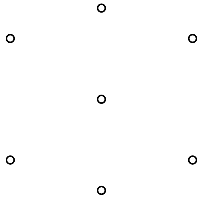
We will prove the lower bound via Theorem 10 with $m=2(r-1)$. Let $H=C_{r}+P_{r-2}$ and $H^{\prime}=P_{2(r-1)}$. Note that $\mathsf{s}(P_{i},H)=\mathsf{s}(P_{i},H^{\prime})=2r-1-i$ for $i=1,2,\dots,r-1$. For an illustration of the construction when $r=5$, see Fig. 6. Since paths of length at most $r-1$ are the only connected subgraphs of $H$ and $H^{\prime}$ with at most $r-1$ vertices, Corollary 1 implies that $H$ and $H^{\prime}$ have matching subgraph counts up to order $r-1$.

(a) The graph $H$

(b) The graph $H^{\prime}$.

Figure 6: The construction for $r=5$. Each connected subgraph with $k\leq 4$ vertices appears exactly $9-k$ times in each graph.

In the notation of Theorem 10, $k=r-1$, $m=2(r-1)$, and $|\mathsf{cc}(H)-\mathsf{cc}(H^{\prime})|=1$. By Theorem 10,

$$\inf_{\widehat{\mathsf{cc}}}\sup_{G\in{\mathcal{G}}(N,r)}\mathbb{P}\left[|\widehat{\mathsf{cc}}-\mathsf{cc}(G)|\geq\Delta\right]\geq 0.10,$$

where

$$\Delta\asymp|\mathsf{cc}(H)-\mathsf{cc}(H^{\prime})|\left({\sqrt{\frac{N}{m{\rm TV}(P_{{\widetilde{H}}},P_{{\widetilde{H}}^{\prime}})}}}\wedge\frac{N}{m}\right)=\left(\sqrt{\frac{N}{m{\rm TV}(P_{{\widetilde{H}}},P_{{\widetilde{H}}^{\prime}})}}\wedge\frac{N}{m}\right).$$

Furthermore, by (31), the total variation between the sampled graphs ${\widetilde{H}}$ and ${\widetilde{H}}^{\prime}$ satisfies

$${\rm TV}(P_{{\widetilde{H}}},P_{{\widetilde{H}}^{\prime}})\leq e^{-\frac{r^{2}}{r-1}(1-2p+\frac{2p}{r})^{2}}\leq e^{-r(1-2p)^{2}}<1/300,$$

provided $p<1/2$ and $r\geq\frac{6}{(1-2p)^{2}}$. The desired lower bound on the squared error follows from Markov’s inequality. ∎

B.3 Lower bounds for forests

Particularizing Theorem 11 to $\omega=2$, we obtain a lower bound which shows that the estimator for forests $\widehat{\mathsf{cc}}={\mathsf{v}}({\widetilde{G}})/p-{\mathsf{e}}({\widetilde{G}})/p^{2}$ proposed by Frank [21] is minimax rate-optimal. As opposed to the general construction in Theorem 11, Fig. 7 illustrates a simple construction of $H$ and $H^{\prime}$ for forests. However, we still require that $p$ is less than some absolute constant. Through another argument, we show that this constant can be arbitrarily close to one.

(a) The graph of $H$ for $\omega=2$ and $m=6$.

(b) The graph of $H^{\prime}$ for $\omega=2$ and $m=6$.

Figure 7: The two graphs are isomorphic if the center vertex is not sampled and all incident edges are removed. Thus, ${\rm TV}(P_{{\widetilde{H}}},P_{{\widetilde{H}}^{\prime}})=p(1-q^{6})$.

Theorem 14 (Forests).

Let $\mathcal{F}(N,d)={\mathcal{G}}(N,d,2)$ denote the collection of all forests on $N$ vertices with maximum degree at most $d$. Then for all $0<p<1$,

$$\inf_{\widehat{\mathsf{cc}}}\sup_{G\in{\mathcal{F}}(N,d)}\mathbb{E}_{G}|\widehat{\mathsf{cc}}-\mathsf{cc}(G)|^{2}\gtrsim\left(\frac{Nq}{p^{2}}\vee\frac{Nqd}{p}\right)\wedge N^{2}.$$

In particular, if $d=\Theta(N)$ and $\omega\geq 2$, then

$$\inf_{\widehat{\mathsf{cc}}}\sup_{G\in{\mathcal{G}}(N,d,\omega)}\mathbb{E}_{G}|\widehat{\mathsf{cc}}-\mathsf{cc}(G)|\geq\inf_{\widehat{\mathsf{cc}}}\sup_{G\in{\mathcal{F}}(N,d)}\mathbb{E}_{G}|\widehat{\mathsf{cc}}-\mathsf{cc}(G)|\gtrsim N.$$

Proof.

The strategy is to choose a one-parameter family of forests ${\mathcal{F}}_{0}$ and reduce the problem to estimating the total number of trials in a binomial experiment with a given success probability. To this end, define $M=N/(d+1)$ and let

$${\mathcal{F}}_{0}=\{(N-m(d+1))S_{0}+mS_{d}:m\in\{0,1,\dots,M\}\}.$$

Let $G\in{\mathcal{F}}_{0}$. Because we do not observe the labels $\{b_{v}:v\in V(G)\}$, the distribution of ${\widetilde{G}}$ can be described by the vector $(T_{0},T_{1},\dots,T_{d})$, where $T_{j}$ is the observed number of $S_{j}$. Since $T_{0}=N-\sum_{j\geq 1}(j+1)T_{j}$, it follows that $(T_{1},\dots,T_{d})$ is sufficient for ${\widetilde{G}}$. Next, we will show that $T=T_{1}+\cdots+T_{d}\sim\mathrm{Bin}(m,p^{\prime})$, where $p^{\prime}\triangleq p(1-q^{d})$ is sufficient for ${\widetilde{G}}$. To this end, note that conditioned on $T=n$, the probability mass function of $(T_{1},\dots,T_{d})$ at $(n_{1},\dots,n_{d})$ is equal to

$$\frac{\mathbb{P}\left[T_{1}=n_{1},\dots,T_{d}=n_{d},T=n\right]}{\mathbb{P}\left[T=n\right]} =\frac{\binom{m}{n}\binom{n}{n_{1},\dots,n_{d}}p^{n_{1}}_{1}\cdots p^{n_{d}}_{d}(1-p^{\prime})^{m-n}}{\binom{m}{n}(p^{\prime})^{n}(1-p^{\prime})^{m-n}}$$

$$=\binom{n}{n_{1},\dots,n_{d}}(p_{1}/p^{\prime})^{n_{1}}\cdots(p_{d}/p^{\prime})^{n_{d}},$$

where $p_{j}\triangleq\binom{d}{j}p^{j}q^{d-j}$. Thus, $(T_{1},\dots,T_{d})\mid T=n\sim\text{Multinomial}(n,p_{1}/p^{\prime},\dots,p_{d}/p^{\prime})$, whose distribution is independent of $m$. Thus, since $\mathsf{cc}(G)=N-md$, we have that

$$\inf_{\widehat{\mathsf{cc}}}\sup_{G\in{\mathcal{F}}(N,d)}\mathbb{E}_{G}|\widehat{\mathsf{cc}}-\mathsf{cc}(G)|^{2} \geq\inf_{\widehat{\mathsf{cc}}}\sup_{G\in{\mathcal{F}}_{0}}\mathbb{E}_{G}|\widehat{\mathsf{cc}}-\mathsf{cc}(G)|^{2}$$

$$=d^{2}\inf_{\widehat{m}(T)}\sup_{m\in\{0,1,\dots,M\}}\mathbb{E}_{T\sim\mathrm{Bin}(m,p^{\prime})}|\widehat{m}(T)-m|^{2}$$

$$\gtrsim\left(\frac{Nq}{p^{2}}\vee\frac{Nqd}{p}\right)\wedge N^{2},$$

which follows applying Lemma 11 below with $\alpha=p^{\prime}$ and $M=N/(d+1)$ and the fact that $p^{\prime}=p(1-q^{d})\leq p\wedge(p^{2}d)$. ∎

The proof of Lemma 11 is given in Appendix A.

Lemma 11 (Binomial experiment).

Let $X\sim\mathrm{Bin}(m,\alpha)$. For all $0\leq\alpha\leq 1$ and $M\in\mathbb{N}$ known a priori,

$$\inf_{\widehat{m}}\sup_{m\in\{0,1,\dots,M\}}\mathbb{E}|\widehat{m}(X)-m|^{2}\asymp\frac{(1-\alpha)M}{\alpha}\wedge M^{2}.$$

Proof.

The upper bound follows from choosing $\widehat{m}=X/\alpha$ when $\alpha>(1-\alpha)/M$ and $\widehat{m}=(M+1)/2$ when $\alpha\leq(1-\alpha)/M$.

For the lower bound, let $\gamma>0$. Consider the two hypothesis $H_{1}:m_{1}=M$ and $H_{2}:m_{2}=M-\sqrt{\frac{\gamma M}{\alpha}}\wedge M$. By Le Cam’s two point method [55, Theorem 2.2(i)],

$$\inf_{\widehat{m}}\sup_{m\in\{0,1,\dots,M\}}\mathbb{E}|\widehat{m}(X)-m|^{2} \geq\frac{1}{2}|m_{1}-m_{2}|^{2}[1-{\rm TV}(\mathrm{Bin}(m_{1},\alpha),\mathrm{Bin}(m_{2},\alpha))]$$

$$\geq\frac{\frac{\gamma M}{\alpha}\wedge M^{2}}{2}[1-H(\mathrm{Bin}(m_{1},\alpha),\mathrm{Bin}(m_{2},\alpha))],$$

where we used the inequality between total variation and the Hellinger distance ${\rm TV}\leq H$ [55, Lemma 2.3]. Finally, choosing $\gamma=(1-\alpha)/16$ and using the bound in [48, Lemma 21] on the Hellinger distance between two binomials, we obtain

$$H(\mathrm{Bin}(m_{1},\alpha),\mathrm{Bin}(m_{2},\alpha))\leq 1/2$$

as desired. ∎

Appendix C Numerical experiments

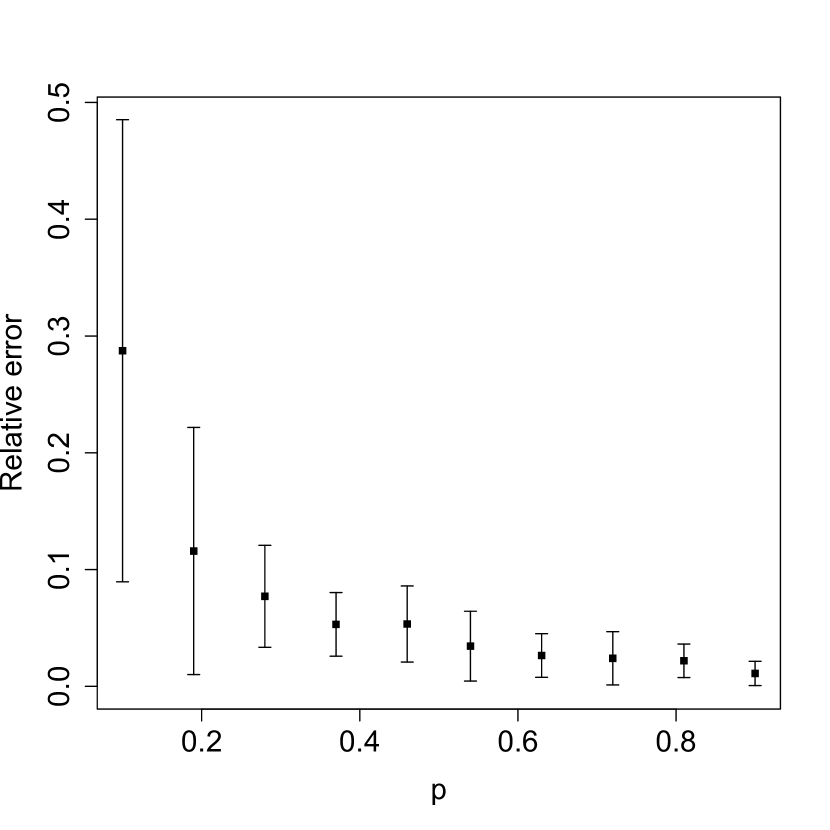
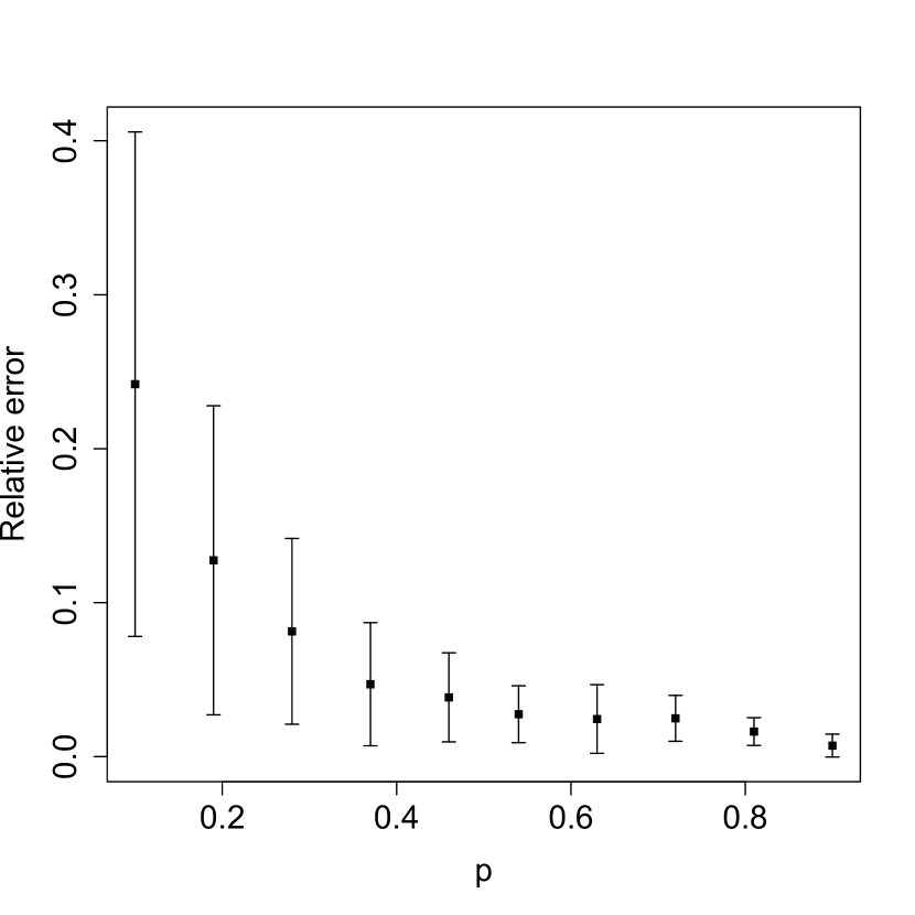
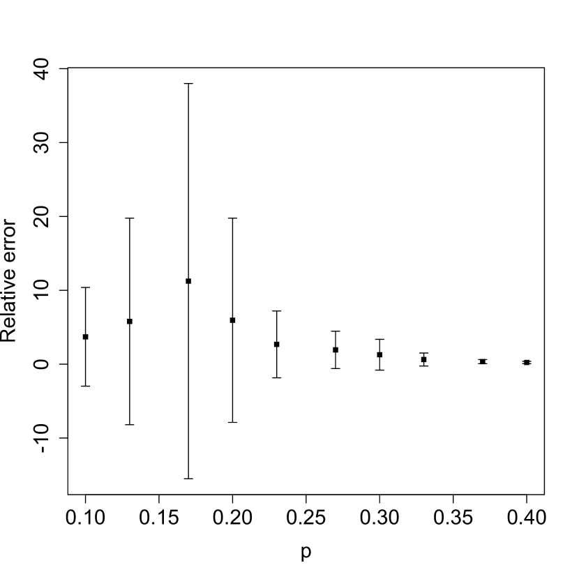
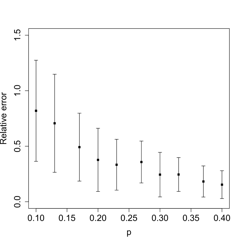
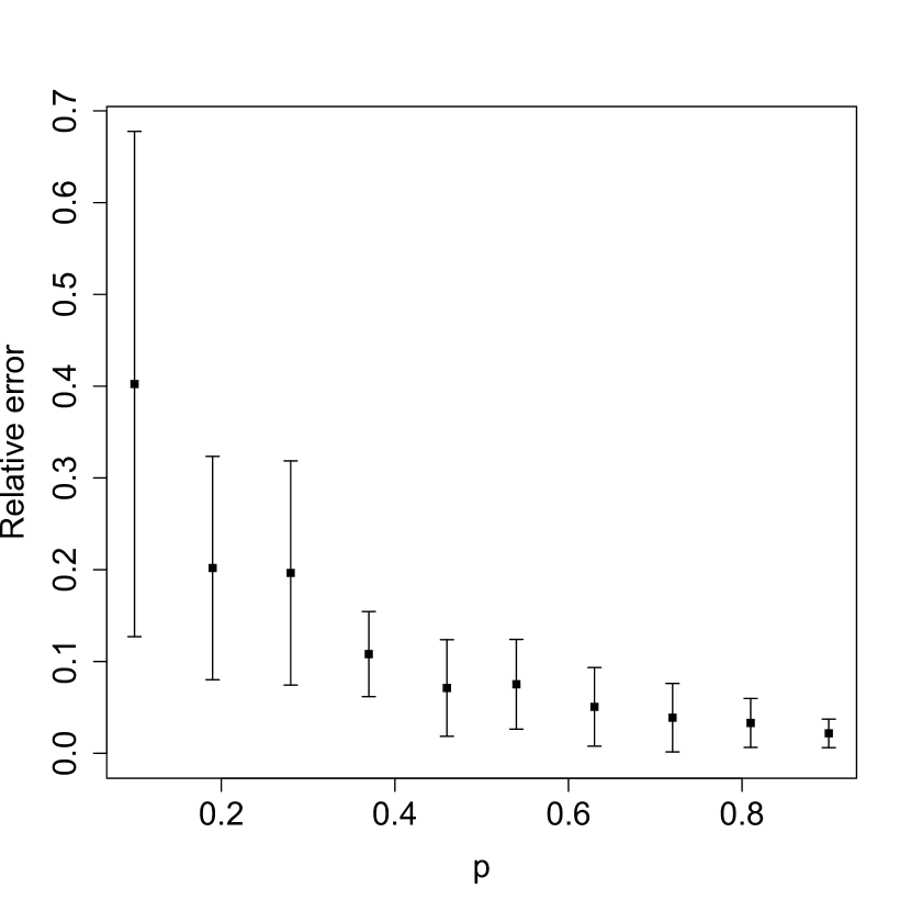
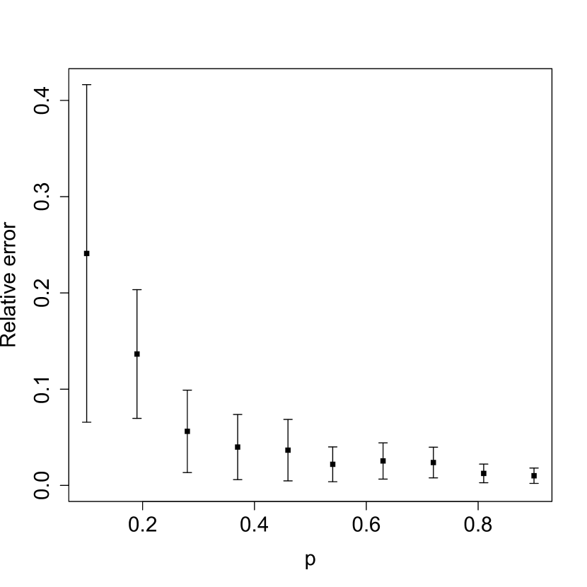
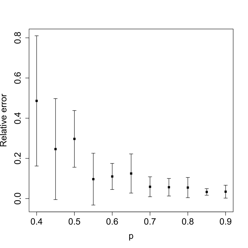
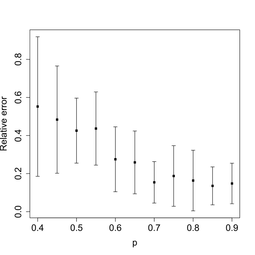
In this section, we study the empirical performance of the estimators proposed in Section 4 using synthetic data from various random graphs. The error bars in the following plots show the variability of the relative error $\frac{|\widehat{\mathsf{cc}}-\mathsf{cc}(G)|}{\mathsf{cc}(G)}$ over 20 independent experiments of subgraph sampling on a fixed parent graph $G$. The solid black horizontal line shows the sample average and the whiskers show the mean $\pm$ the standard deviation.

C.1 Synthetic experiment

Chordal graphs

Both Fig. 8 and Fig. 9 focus on chordal graphs, where the parent graph is first generated from a random graph ensemble then triangulated by calculating a fill-in of edges to make it chordal (using a maximum cardinality search algorithm from [54]). In Fig. 8(a), the parent graph $G$ is a triangulated Erdös-Rényi graph ${\mathcal{G}}(N,\delta)$, with $N=2000$ and $\delta=0.0005$ which is below the connectivity threshold $\delta=\frac{\log N}{N}$ [16]. In Fig. 8(b), we generate $G$ with $N=20000$ vertices by taking the disjoint union of 200 independent copies of ${\mathcal{G}}(100,0.2)$ and then apply triangulation. In accordance with Theorem 6, the better performance in Fig. 8(b) is due to moderately sized $d$ and $\omega$, and large $\mathsf{cc}(G)$.

In Fig. 9 we perform a simulation study of the smoothed estimator $\widehat{\mathsf{cc}}_{L}$ from Theorem 7. The parent graph is equal to a triangulated realization of ${\mathcal{G}}(1000,0.0015)$ with $d=88$, $\omega=15$, and $\mathsf{cc}(G)=325$. The plots in Fig. 11(b) show that the sampling variability is significantly reduced for the smoothed estimator, particularly for small values of $p$ (to show detail, the vertical axes are plotted on different scales). This behavior is in accordance with the upper bounds furnished in Theorem 6 and Theorem 7. Large values of $\omega$ inflate the variance of $\widehat{\mathsf{cc}}$ considerably by an exponential factor of $1/p^{\omega}$, whereas the effect of large $\omega$ on the variance of $\widehat{\mathsf{cc}}_{L}$ is polynomial, viz., $\omega^{\frac{p}{2-3p}}$. We chose the smoothing parameter $\lambda$ to be $p\log N$, but other values that improve the performance can be chosen through cross-validation on various known graphs.

The non-monotone behavior of the relative error in Fig. 11(a) can be explained by the tradeoff between increasing $p$ (which improves the accuracy) and increasing probability of observing a clique (which increases the variability, particularly in this case of large $\omega$). Such behavior is apparent for moderate values of $p$ (e.g., $p<0.25$), but less so as $p$ increases to $1$ since the mean squared error tends to zero as more of the parent graph is observed. The plots also suggest that the marginal benefit (i.e., the marginal decrease in relative error) from increasing $p$ diminishes for moderate values of $p$. Future research would address the selection of $p$, if such control was available to the experimenter.

Non-chordal graphs

Finally, in Fig. 10 we experiment with sampling non-chordal graphs. As proposed in Section 4.4, one heuristic is to modify the original estimator by first triangulating the subsampled graph ${\widetilde{G}}$ to $\mathsf{TRI}({\widetilde{G}})$ and then applying the estimator $\widehat{\mathsf{cc}}$ in (10). The plots in Fig. 10 show that this strategy works well; in fact the performance is competitive with the same estimator in Fig. 8, where the parent graph is first triangulated and then subsampled.

(a) Parent graph equal to a triangulated realization of ${\mathcal{G}}(2000,0.0005)$ with $d=36$, $\omega=5$, and $\mathsf{cc}(G)=985$.

(b) Parent graph equal to a triangulated realization of 200 copies of ${\mathcal{G}}(100,0.2)$ with $d=8$, $\omega=4$, and $\mathsf{cc}(G)=803$.

Figure 8: The relative error of $\widehat{\mathsf{cc}}$ with moderate values of $d$ and $\omega$.

(a) Non-smoothed $\widehat{\mathsf{cc}}$.

(b) Smoothed $\widehat{cc}_{L}$.

Figure 9: A comparison of the relative error of the unbiased estimator $\widehat{\mathsf{cc}}$ in (10) and its smoothed version $\widehat{\mathsf{cc}}_{L}$ in (25). The parent graph is a triangulated realization of ${\mathcal{G}}(1000,0.0015)$ with $d=88$, $\omega=15$, and $\mathsf{cc}(G)=325$.

(a) Parent graph equal to a realization of ${\mathcal{G}}(2000,0.0005)$ with $d=8$, $\omega=3$, and $\mathsf{cc}(G)=756$.

(b) Parent graph equal to a realization of 200 copies of ${\mathcal{G}}(100,0.2)$ with $d=7$, $\omega=4$, and $\mathsf{cc}(G)=532$.

Figure 10: The estimator $\widehat{\mathsf{cc}}(\mathsf{TRI}({\widetilde{G}}))$ applied to non-chordal graphs.

C.2 Real-data experiment

The point of developing a theory for graphs with specific structure (i.e. chordal) is to (a) study how the graph parameters (such as maximal degree) impact the estimation difficulty and (b) motivate a heuristic for real-world graphs encountered in practice. Indeed, as with all problems in a minimax framework, a certain amount of finesse is required to define a parameter space that showcases the richness of the problem, while at the same time, enables one to provide a characterization of the fundamental limits of estimation. Chordal graphs seem to fit this purpose. Importantly, they serve as a catalyst for more general strategies that apply to a wider collection of parent graphs, including those commonly encountered in practice.

In the previous subsection, we studied the estimators $\widehat{\mathsf{cc}}$ and $\widehat{\mathsf{cc}}_{L}$ using synthetic data on moderately sized, chordal parent graphs. In this section, we consider real-world instances of network datasets, where the parent graph is not chordal and the number of nodes is large. More specifically, we consider two representative examples of collaboration and biological networks. We believe these examples show the usefulness of our estimators on real-world data, despite the fact that the methodology was developed for chordal parent graphs.

The first network [40] is the collaboration network of authors with arXiv “cond-mat” (condense matter physics) articles submitted between January 1993 and April 2003. Note that the category has been active since April 1992. An edge is attached between two researchers in the network if and only if they co-authored a paper together.

The second network [51, Supplementary Table S2] is an initial version of a proteome-scale map of human binary protein-protein interactions (i.e., edges represent direct physical interactions between two protein molecules). Because self-loops do not affect the connectivity of the network, we removed them from the dataset.

We use the smoothed estimator $\widehat{\mathsf{cc}}_{L}$ on both networks; the standard estimator $\widehat{\mathsf{cc}}$ performs poorly because of high-degree vertices and large clique numbers (c.f., Fig. 9). To deal with the non-chordal parent graphs, we again use the heuristic proposed in Section 4.4 of first triangulating the subsampled graph ${\widetilde{G}}$ to $\mathsf{TRI}({\widetilde{G}})$ and then applying the smoothed estimator $\widehat{\mathsf{cc}}_{L}$ in (25). The results of this estimation scheme on both networks are displayed in Fig. 11.

(a) Collaboration network of arXiv condense matter physics: $N=23133$, ${\mathsf{e}}(G)=93439$, $d=279$, and $\mathsf{cc}(G)=567$.

(b) Human protein-protein network: $N=3133$, ${\mathsf{e}}(G)=6149$, $d=129$, and $\mathsf{cc}(G)=210$.

Figure 11: Smoothed estimator $\widehat{\mathsf{cc}}_{L}(\mathsf{TRI}({\widetilde{G}}))$ applied to a collaboration and biological network.

References

- [1] Milton Abramowitz and Irene A. Stegun, editors. Handbook of mathematical functions with formulas, graphs, and mathematical tables. Dover Publications, Inc., New York, 1992. Reprint of the 1972 edition.
- [2] Maryam Aliakbarpour, Amartya Shankha Biswas, Themis Gouleakis, John Peebles, Ronitt Rubinfeld, and Anak Yodpinyanee. Sublinear-time algorithms for counting star subgraphs via edge sampling. Algorithmica, pages 1–30, 2017.
- [3] Coren L. Apicella, Frank W. Marlowe, James H. Fowler, and Nicholas A. Christakis. Social networks and cooperation in hunter-gatherers. Nature, 481(7382):497–501, 01 2012.
- [4] Oriana Bandiera and Imran Rasul. Social networks and technology adoption in northern Mozambique. The Economic Journal, 116(514):869–902, 2006.
- [5] Anna Ben-Hamou, Roberto I Oliveira, and Yuval Peres. Estimating graph parameters via random walks with restarts. arXiv preprint arXiv:1709.00869, 2017.
- [6] Petra Berenbrink, Bruce Krayenhoff, and Frederik Mallmann-Trenn. Estimating the number of connected components in sublinear time. Inform. Process. Lett., 114(11):639–642, 2014.
- [7] C. Borgs, J. T. Chayes, L. Lovász, V. T. Sós, and K. Vesztergombi. Convergent sequences of dense graphs. I. Subgraph frequencies, metric properties and testing. Adv. Math., 219(6):1801–1851, 2008.
- [8] Michael Capobianco. Estimating the connectivity of a graph. Graph Theory and Applications, pages 65–74, 1972.
- [9] Arun Chandrasekhar and Randall Lewis. Econometrics of sampled networks. Unpublished manuscript, 2011.
- [10] Bernard Chazelle, Ronitt Rubinfeld, and Luca Trevisan. Approximating the minimum spanning tree weight in sublinear time. SIAM J. Comput., 34(6):1370–1379, 2005.
- [11] Beidi Chen, Anshumali Shrivastava, and Rebecca C Steorts. Unique entity estimation with application to the Syrian conflict. arXiv preprint arXiv:1710.02690, 2017.
- [12] Timothy G. Conley and Christopher R. Udry. Learning about a new technology: Pineapple in ghana. American Economic Review, 100(1):35–69, March 2010.
- [13] Graham Cormode and Nick Duffield. Sampling for big data: a tutorial. In Proceedings of the 20th ACM SIGKDD International Conference on Knowledge Discovery and Data Mining, pages 1975–1975. ACM, 2014.
- [14] Klaus Dohmen. Lower bounds for the probability of a union via chordal graphs. Electronic Communications in Probability, 18, 2013.
- [15] Talya Eden, Amit Levi, Dana Ron, and C. Seshadhri. Approximately counting triangles in sublinear time. In 2015 IEEE 56th Annual Symposium on Foundations of Computer Science—FOCS 2015, pages 614–633. IEEE Computer Soc., Los Alamitos, CA, 2015.
- [16] P. Erdös and A. Rényi. On the evolution of random graphs. Magyar Tud. Akad. Mat. Kutató Int. Közl., 5:17–61, 1960.
- [17] Paul Erdös, László Lovász, and Joel Spencer. Strong independence of graphcopy functions. In Graph theory and related topics (Proc. Conf., Univ. Waterloo, Waterloo, Ont., 1977), pages 165–172. Academic Press, New York-London, 1979.
- [18] Marcel Fafchamps and Susan Lund. Risk-sharing networks in rural Philippines. Journal of development Economics, 71(2):261–287, 2003.
- [19] Benjamin Feigenberg, Erica M Field, and Rohini Pande. Building social capital through microfinance. Technical report, National Bureau of Economic Research, 2010.
- [20] Ove Frank. Estimation of graph totals. Scand. J. Statist., 4(2):81–89, 1977.
- [21] Ove Frank. Estimation of the number of connected components in a graph by using a sampled subgraph. Scand. J. Statist., 5(4):177–188, 1978.
- [22] Chao Gao, Yu Lu, and Harrison H Zhou. Rate-optimal graphon estimation. The Annals of Statistics, 43(6):2624–2652, 2015.
- [23] Oded Goldreich. Introduction to Property Testing. Cambrdige University, 2017.
- [24] Oded Goldreich, Shari Goldwasser, and Dana Ron. Property testing and its connection to learning and approximation. Journal of the ACM (JACM), 45(4):653–750, 1998.
- [25] Oded Goldreich and Dana Ron. Approximating average parameters of graphs. Random Structures Algorithms, 32(4):473–493, 2008.
- [26] Oded Goldreich and Dana Ron. On testing expansion in bounded-degree graphs. In Studies in Complexity and Cryptography. Miscellanea on the Interplay between Randomness and Computation, pages 68–75. Springer, 2011.
- [27] Leo A. Goodman. On the estimation of the number of classes in a population. Ann. Math. Statistics, 20:572–579, 1949.
- [28] Leo A. Goodman. Snowball sampling. Ann. Math. Statist., 32:148–170, 1961.
- [29] Ramesh Govindan and Hongsuda Tangmunarunkit. Heuristics for internet map discovery. In INFOCOM 2000. Nineteenth Annual Joint Conference of the IEEE Computer and Communications Societies. Proceedings. IEEE, volume 3, pages 1371–1380. IEEE, 2000.
- [30] Mark S. Handcock and Krista J. Gile. Modeling social networks from sampled data. Ann. Appl. Stat., 4(1):5–25, 2010.
- [31] Paul W Holland, Kathryn Blackmond Laskey, and Samuel Leinhardt. Stochastic blockmodels: First steps. Social networks, 5(2):109–137, 1983.
- [32] Paul W Holland and Samuel Leinhardt. An exponential family of probability distributions for directed graphs. Journal of the American Statistical Association, 76(373):33–50, 1981.
- [33] Daniel G Horvitz and Donovan J Thompson. A generalization of sampling without replacement from a finite universe. Journal of the American Statistical Association, 47(260):663–685, 1952.
- [34] Svante Janson. Large deviations for sums of partly dependent random variables. Random Structures Algorithms, 24(3):234–248, 2004.
- [35] Jason M. Klusowski and Yihong Wu. Counting motifs with graph sampling. In Proceedings of the 31st Conference On Learning Theory, pages 1966–2011, 2018.
- [36] W. L. Kocay. Some new methods in reconstruction theory. In Combinatorial mathematics, IX (Brisbane, 1981), volume 952 of Lecture Notes in Math., pages 89–114. Springer, Berlin-New York, 1982.
- [37] Eric D Kolaczyk. Statistical Analysis of Network Data: Methods and Models. Springer Science & Business Media, 2009.
- [38] Eric D. Kolaczyk. Topics at the Frontier of Statistics and Network Analysis: (Re)Visiting the Foundations. SemStat Elements. Cambridge University Press, 2017.
- [39] Jure Leskovec and Christos Faloutsos. Sampling from large graphs. In Proceedings of the 12th ACM SIGKDD International Conference on Knowledge Discovery and Data Mining, pages 631–636. ACM, 2006.
- [40] Jure Leskovec and Andrej Krevl. SNAP Datasets: Stanford large network dataset collection. http://snap.stanford.edu/data/ca-CondMat.html, June 2014.
- [41] László Lovász. Large Networks and Graph Limits, volume 60. American Mathematical Society, 2012.
- [42] R Duncan Luce and Albert D Perry. A method of matrix analysis of group structure. Psychometrika, 14(2):95–116, 1949.
- [43] Brendan D. McKay and Stanisław P. Radziszowski. Subgraph counting identities and Ramsey numbers. J. Combin. Theory Ser. B, 69(2):193–209, 1997.
- [44] Elizabeth W. McMahon, Beth A. Shimkus, and Jessica A. Wolfson. Chordal graphs and the characteristic polynomial. Discrete Math., 262(1-3):211–219, 2003.
- [45] Assaf Natanzon, Ron Shamir, and Roded Sharan. A polynomial approximation algorithm for the minimum fill-in problem. SIAM J. Comput., 30(4):1067–1079, 2000.
- [46] Ryan O’Donnell. Analysis of Boolean functions. Cambridge University Press, New York, 2014.
- [47] Alon Orlitsky, Ananda Theertha Suresh, and Yihong Wu. Optimal prediction of the number of unseen species. Proc. Natl. Acad. Sci. USA, 113(47):13283–13288, 2016.
- [48] Yury Polyanskiy, Ananda Theertha Suresh, and Yihong Wu. Sample complexity of population recovery. In Proceedings of Conference on Learning Theory (COLT), Amsterdam, Netherland, Jul 2017. arXiv:1702.05574.
- [49] Peter H Reingen and Jerome B Kernan. Analysis of referral networks in marketing: Methods and illustration. Journal of Marketing Research, pages 370–378, 1986.
- [50] Donald J. Rose, R. Endre Tarjan, and George S. Lueker. Algorithmic aspects of vertex elimination on graphs. SIAM J. Comput., 5(2):266–283, 1976.
- [51] Jean-François Rual, Kavitha Venkatesan, Tong Hao, Tomoko Hirozane-Kishikawa, Amélie Dricot, Ning Li, Gabriel F Berriz, Francis D Gibbons, Matija Dreze, Nono Ayivi-Guedehoussou, et al. Towards a proteome-scale map of the human protein–protein interaction network. Nature, 437(7062):1173, 2005.
- [52] Matthew J Salganik and Douglas D Heckathorn. Sampling and estimation in hidden populations using respondent-driven sampling. Sociological methodology, 34(1):193–240, 2004.
- [53] Michael PH Stumpf, Thomas Thorne, Eric de Silva, Ronald Stewart, Hyeong Jun An, Michael Lappe, and Carsten Wiuf. Estimating the size of the human interactome. Proceedings of the National Academy of Sciences, 105(19):6959–6964, 2008.
- [54] Robert E. Tarjan and Mihalis Yannakakis. Simple linear-time algorithms to test chordality of graphs, test acyclicity of hypergraphs, and selectively reduce acyclic hypergraphs. SIAM J. Comput., 13:566–579, 1984.
- [55] Alexandre B. Tsybakov. Introduction to nonparametric estimation. Springer Series in Statistics. Springer, New York, 2009. Revised and extended from the 2004 French original, Translated by Vladimir Zaiats.
- [56] Douglas B. West. Introduction to graph theory. Prentice Hall, Inc., Upper Saddle River, NJ, 1996.
- [57] Hassler Whitney. The coloring of graphs. Ann. of Math. (2), 33(4):688–718, 1932.
- [58] Yihong Wu and Pengkun Yang. Sample complexity of the distinct element problem. arxiv preprint arxiv:1612.03375, Apr 2016.