Hydrodynamic heat transport regime in bismuth : a theoretical viewpoint

Abstract

Bismuth is one of the rare materials in which second sound has been experimentally observed. Our exact calculations of thermal transport with the Boltzmann equation predict the occurrence of this Poiseuille phonon flow between $\approx$ 1.5 K and $\approx$ 3.5 K, in sample size of 3.86 mm and 9.06 mm, in consistency with the experimental observations. Hydrodynamic heat flow characteristics are given for any temperature : heat wave propagation length, drift velocity, Knudsen number. We discuss a Gedanken experiment allowing to assess the presence of a hydrodynamic regime in any bulk material.

Currently a lot of attention is devoted to the study of phonon-based heat transport regimes in nanostructures Cahill et al. (2015); Volz et al. (2016); Chang et al. (2008); Yand et al. (2010). Of particular interest is the hydrodynamic regime in which a number of fascinating phenomena such as Poiseuille’s phonon flow and second sound occur, and where temperature fluctuations are predicted to propagate as a true temperature wave of the form $e^{i(\mathbf{k}\cdot\mathbf{r}-\omega t)}$ Guo and Wang (2015). The theoretical study of the hydrodynamic regime has encountered a renewed interest in graphene nanoribbons, where the breakdown of the diffusive Fourier law in favor of the second sound propagation has been predicted Zhang et al. (2011); Fugallo et al. (2014); Lee et al. (2015); Cepellotti et al. (2015). Bismuth has the particularity to be a semimetal with relatively low carrier concentrations so that the dominant mechanism for heat conduction at low temperatures is via phonons Narayanamurti and Dynes (1972); Issi (1979). Together with solid helium Ackerman et al. (1966) and NaF Jackson et al. (1970), it is one of the rare materials that are sufficiently isotopically pure so that second sound could be observed. The degree of physical and chemical perfection that has been achieved in Bi crystals is so high that also transitions between the various regimes have been experimentally observed with the increase of the (yet cryogenic) temperature : from heat transport via ballistic phonons, to the regime of Poiseuille’s flow with second sound, to the diffusive (Fourier) propagation Narayanamurti and Dynes (1972).

Neither the conditions for the occurrence of the hydrodynamic regime nor the transition temperatures have ever been supported by a theoretical work in one of the above-cited 3-D materials. So far, phonon hydrodynamics has been studied with the lattice Boltzmann formalism for a model dielectric material with an ad hoc three-phonon collision term and no resistive processes Guyer (1994). The transition to the kinetic regime has been modeled in group IV semiconductors through a hydrodynamic-to-kinetic switching factor proportional to the ratio of normal and resistive scattering rates de Tomas et al. (2014a, b); de Tomas et al. (2015). A review on advances in phonon hydrodynamics points out the lack of a widely applicable hydrodynamic model which would consider all of the normal and resistive processes Guo and Wang (2015).

In this work, a major advance consists in accounting for the phonon repopulation by the normal processes in the framework of the exact variational solution of the Boltzmann transport equation (V-BTE) Omini and Sparavigna (1995); Fugallo et al. (2013), coupled to the ab initio description of anharmonicity : three-phonon collisions turn out to be particularly strong at low temperatures, and lead to the creation of new phonons in the direction of the heat flow (normal processes) which enhance the heat transport. This induces time- and length-scales over which heat carriers behave collectively and form a hydrodynamic flow that cannot be described by independent phonons with their own energy and lifetime. In other words the single mode approximation (SMA), valid for the phonon gas model, breaks down. The resistive processes are entirely controlled by few phonon-phonon anharmonic processes which lead to the creation of phonons in the direction opposite to the heat flow (Umklapp processes), and by extrinsic processes coming from phonon scattering by the sample boundaries.

The characterization of heat transport regimes, and in particular of the transition between the hydrodynamic and kinetic regimes, is the main focus of present work. We discuss several methods to define the hydrodynamic regime, and provide the link with macroscopic scale quantities Guo and Wang (2015) like Knudsen number and drift velocity. In particular, we extract the heat wave propagation length (HWPL) directly from the lattice thermal conductivity (LTC) calculated with V-BTE. We argue that our method to extract the HWPL from the LTC in samples of different sizes, combined to a measurement of the average phonon mean free path, can be viewed as a Gedanken experiment which could allow to determine the transition from the hydrodynamic to kinetic regime in any material.

Several criteria are used in order to identify the hydrodynamic to kinetic transition. First, the picture of the heat carried by single (uncorrelated) phonons with finite lifetimes, is valid in the kinetic regime only. Thus, a significant difference between the LTC obtained by a solution of V-BTE and the one obtained in the single mode approximation (SMA-BTE) is the indication that the hydrodynamic regime is achieved. Second, we compare the thermodynamic averages of the phonon-scattering rates for normal and resistive processes $\Gamma^{n}$ and $\Gamma^{U}$, and the hydrodynamic regime occurs when Guyer and Krumhansl (1966)

$$\Gamma^{U}_{av}\ll\Gamma^{n}_{av}.$$ (1)

Then, we address the question of the occurrence of Poiseuille’s flow inside the hydrodynamic regime. Here as well, various methods are employed, which now account for the additional scattering rate by sample boundaries $\Gamma^{b}$. We first use Guyer’s conditions Guyer and Krumhansl (1966),

$$\Gamma^{U}_{av}\,\,<\,\,\Gamma^{b}_{av}\,\,<\,\,\Gamma^{n}_{av}\,$$ (2)

and find the temperature interval in which second-sound is calculated to be observable. In the second method, we extract the heat wave propagation length directly from the LTC calculated with V-BTE and compare it to the sample size which sets the threshold for the second sound observability. Above the threshold, the heat-wave is damped before reaching the sample boundary.

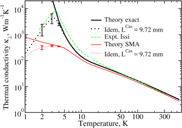
Figure 1: Temperature dependence of the LTC in the binary direction for a single crystal without (solid lines) or with (dotted lines) millimeter-sized sample boundaries (MSSB). Black curves : exact variational calculation (V-BTE). Red curves : single mode approximation (SMA-BTE). MSSB modeled with the wire geometry and $L^{\mathrm{Cas}}$ $=$ 9.72 mm Mar (a). Green dashed lines : LTC extracted by us from expt. of Ref. Uher and Goldsmid, 1974 for $T>20$ K; for $T<20$ K, LTC from a sample having a rectangular cross-section $8.8\times 8.6$ mm² (Ref. Issi, 1979). We used the T-independent bulk value of 6 W(K.m)^-1 Markov et al. (2016); Markov (2016) of the electronic contribution to extract the LTC from the total thermal conductivity of Bi Issi (1979). The error bar in our calculations results from the variation of the geometrical factor $\frac{1}{F}$=2$\pm$1.

The thermodynamic averages of phonon scattering rates for normal, Umklapp and boundary collisional processes that condition the transport regime read

$$\Gamma^{i}_{av}=\frac{\sum_{\nu}C_{\nu}\Gamma_{\nu}^{i}}{\sum_{\nu}C_{\nu}}$$ (3)

where $C_{\nu}$ is the specific heat (see below) of the phonon mode $\nu=\{\mathbf{q}j\}$ and the index $i=n,U,b$ stands for normal, Umklapp and extrinsic (boundary) scattering respectively. Besides the scattering rate (or inverse relaxation time), the quantities characterizing heat transport are the drift velocity $v$ of the heat carriers defined below, and the phonon propagation length $\lambda=v\,\Gamma_{av}^{-1}$ which is the characteristic distance that heat carrying phonons cover before damping. As a source of damping, we consider, in infinite samples, either Umklapp processes only

$$\lambda_{hydro}(\infty)=v/\Gamma_{av}^{U},$$ (4)

or their combination with normal processes through Matthiessen’s rule

$$\lambda_{gas}(\infty)=v/(\Gamma_{av}^{U}+\Gamma_{av}^{n})\,.$$ (5)

When scattering by sample boundaries is accounted for, the phonon propagation length reads $\lambda(L^{\mathrm{Cas}})$ instead of $\lambda(\infty)$ in eqs. 4$-$5, where Casimir’s length $L^{\mathrm{Cas}}$ represents the smallest dimension of the sample or nanostructure.

In bismuth the transport is anisotropic and has components along the trigonal axis ($\parallel$) and perpendicular ($\perp$) to it, i.e. along the binary and bisectrix directions. The drift velocity in these directions reads Cepellotti et al. (2015)

$$v_{j}^{2}=\frac{\sum_{\nu}C_{\nu}\,\,\mathbf{c}_{\nu\,j}\cdot\mathbf{c}_{\nu\,j}}{\sum_{\nu}C_{\nu}},$$ (6)

where $j$ stands for $\parallel$ or $\perp$ direction and $\mathbf{c}_{\nu}$ is the phonon group velocity. In the thermodynamic averages the specific heat of a phonon mode is calculated as $C_{\nu}$ = $n_{\nu}^{0}(n_{\nu}^{0}+1)\frac{(\hbar\omega_{\nu})^{2}}{k_{B}T^{2}}$, where $n^{0}$ stands for the temperature (T) dependent Bose-Einstein phonon occupation number and $\omega_{\nu}$ is the phonon frequency.

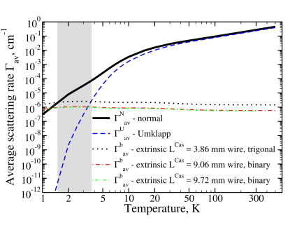
Figure 2: Temperature dependence of the thermodynamic average of the anharmonic scattering rates for normal and Umklapp processes (resp. black solid and blue dashed line) and of the (boundary) extrinsic scattering rates (ESR) (dashed black and dot-dashed red and green lines). ESR have been calculated for a wire geometry using $L^{\mathrm{Cas}}$ $=$ $3.86$ mm Mar (b) and $L^{\mathrm{Cas}}=9.06$ mm Mar (c), and with $L^{\mathrm{Cas}}$ $=$ $9.72$ mm Mar (a) as in Fig 1. ESR for $L^{\mathrm{Cas}}$ $=$ $9.06$ and $L^{\mathrm{Cas}}$ $=$ $9.72$ mm are hardly distinguishable on the scale of the figure. The shaded region corresponds to the temperature interval in which a second sound peak has been reported, 1.5 K $<T<$ 3.5 K for a sample of length 3.86 mm in the trigonal propagation direction Narayanamurti and Dynes (1972).

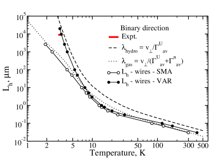
Figure 3: Heat wave propagation length $L_{h}$ extracted from the LTC calculations in the binary direction as a function of temperature. Solid line with black filled disks : $L_{h}$ obtained with V-BTE, accounting for phonon repopulation. Solid line with empty circles : $L_{h}$ obtained with SMA-BTE. Black dashed line : phonon propagation length $\lambda_{hydro}$ of eq. 4. Black dotted line : phonon propagation length $\lambda_{gas}$ of eq. 5. The red line segment marks the ranges of temperatures, from 3.0 K to 3.48 K, and sample dimension, 9.06 mm, in which a second sound peak has been reported in the binary direction  Narayanamurti and Dynes (1972).

The LTC, third-order anharmonic constants of the normal and Umklapp phonon interactions, and thermodynamical averages have been calculated on a 28x28x28 q-point grid in the Brillouin zone, but for the drift velocity below 2 K, which required a 40$\times$40$\times$40 grid. Details of the calculation are given in the supplemental material. We have used the wire geometry for boundary scattering with Casimir’s model, $\Gamma^{b}=\frac{n^{0}_{\nu}(n^{0}_{\nu}+1)|\mathbf{c}_{\nu}^{b}|}{F\,L^{\mathrm{Cas}}}$, where $\mathbf{c}_{\nu}^{b}$ is the group-velocity in the direction of the smallest dimension. Specularity Berman et al. (1955); Rajabpour et al. (2011); Bourgeois et al. (2016) is neglected and $\frac{1}{F}$ accounts for the geometrical ratio of $L^{\mathrm{Cas}}$ over the finite (yet large) dimension along the heat transport direction Sparavigna (2002a); Fugallo et al. (2013); Markov et al. (2016); Markov (2016); Mar (d). Varying $\frac{1}{F}$ by 2 $\pm$ 1 (Fig. 1) has little consequence on $\kappa_{\perp}$ above T=2 K.

Remarkably, our calculated LTC shows the same evolution as the experimental one over three orders of magnitude (Fig. 1, resp. black dotted and green dashed lines), and the various regimes of heat transport are excellently described from ambient temperature down to 2 K. The LTC increases as $T^{-1}$ with the decrease of temperature down to 10 K. Then in the absence of scattering other than phonon-phonon interaction, the LTC shows an exponential growth below 10 K (black solid line). This behavior is directly due to the weakness of resistive (Umklapp) processes.

The account for boundary scattering makes the LTC value remain finite even in the asymptotic limit. Moreover, the theoretical curves satisfactorily explain the experimental behavior of the LTC and in particular, the position of the conductivity maximum, $T^{max}$, which is found to be 3.2 K for the 9.72 mm wire, in extremely satisfactory agreement with the maximum at 3.6 K observed in experiment (Fig. 1, resp. black dotted and green dashed lines). Further decrease of temperature leads to a decrease of the LTC with a decay law gradually approaching the T³ behavior expected for a regime in which boundary scattering dominates.

The first sign of the transition from the kinetic to hydrodynamic regime around 3 K in infinite samples is demonstrated in Fig. 1 by a large $(>10^{2})$ difference between our V- and SMA-BTE results for the LTC (resp. black and red solid lines). This result shows that the repopulation of phonon states due to normal processes plays an important role, invalidating the SMA picture in which individual phonons have lifetimes and propagation lengths determined by all of the collisional processes (normal and Umklapp, eq. 5). The same conclusion can be drawn by considering Fig. 2 where, around 3 K, normal processes dominate over the resistive ones (Umklapp) by more than one order of magnitude, so that eq. 1 is fulfilled.

The same difference in the LTC between V- and SMA-BTE is found in presence of sample boundaries (Fig. 1, resp. black and red dotted lines) and, remarkably, the average extrinsic scattering rate $\Gamma^{b}_{av}$ calculated with Casimir’s length $L^{\mathrm{Cas}}$ $=$ $3.86$ mm (Fig. 2, black dotted line) lays in between the average normal $\Gamma^{n}_{av}$ and Umklapp $\Gamma^{U}_{av}$ scattering rates and thus, satisfy the criterion of eq. 2 for the existence of Poiseuille’s flow and second sound observability Guyer and Krumhansl (1966). The temperature interval calculated with eq. 2 is 1.5 K $<T<$ 3.6 K, in perfect agreement with the temperature range, 1.5 K$<T<$3.5 K, in which second sound has been observed experimentally in the trigonal direction (grey shaded region) Narayanamurti and Dynes (1972). For $L^{\mathrm{Cas}}=9.06$ mm in the binary direction (red dot-dashed line), the calculated interval is 1.3 K $<T<$ 3.4 K, a temperature range slightly more extended than the experimental one, 3.0 K$<T<$3.48 K Narayanamurti and Dynes (1972). In our calculations, Poiseuille’s regime ends for temperatures lower than 1.5 K, where phonon scattering by sample boundaries becomes significant (Fig. 2).

However, the average scattering rates discussed so far do not contain any information about repopulation mechanisms Mar (e) . To account for them, we extract a heat wave propagation length $L_{h}$ that we define by the criterion :

$$\kappa(T,L^{\mathrm{Cas}}=L_{h})=\kappa(T,\infty)/e,$$ (7)

where $\kappa(T,\infty)$ denotes the LTC obtained for an infinite sample at a given temperature, and $\kappa(T,L^{\mathrm{Cas}})$ denotes the LTC obtained for a sample of finite dimension. The extracted HWPL $L_{h}$ is the cylindrical wire diameter $L^{\mathrm{Cas}}$ needed to reduce $\kappa(T,\infty)$ by $e$ (Fig. 3, filled disks, and supplemental material for the trigonal direction Mar (f)).

Remarkably, at low temperatures, $L_{h}$ is found to be close to the phonon propagation length computed with Umklapp processes only (eq. 4). These resistive processes damp the heat wave, thus defining the wave traveling distance between the instant of heat wave generation to complete diffusion. A strong presence of normal processes, in turn, favors heat conduction and second sound behavior. With the increase of temperature, $L_{h}$ becomes close to the phonon propagation length accounting for both Umklapp and normal processes of eq. 5, i.e. of an uncorrelated phonon gas (empty circles). We see that the behavior of $L_{h}$ as a function of temperature is the fingerprint of the transition from the hydrodynamic to kinetic regime. The temperature range and sample dimension in which observations of second sound are available in the binary direction (red line segment) are in extremely satisfactory agreement with the calculations, which support the occurrence of second sound at 3.0 K for a 9.72 mm wire. Fig. 3 enables us also to predict the occurrence of second sound at other temperatures and sample sizes, for instance at 4.1 K in a 1 mm size wire.

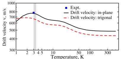
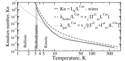
Figure 4: Heat flow characteristics in Bi as a function of the temperature. Panel (a) : drift velocity $v$ in the binary ($\perp$) and trigonal ($\parallel$) directions (resp. black solid and red dashed lines). Symbol : saturated second-sound velocity measured at 3 K Narayanamurti and Dynes (1972). Panel (b) : Knudsen number $L_{h}$/$L^{\mathrm{Cas}}$ for a wire of Casimir’s length $L^{\mathrm{Cas}}$ $=$ $9.72$ mm (black solid line). The ratio of the phonon propagation length in the hydrodynamic (resp. gas) regime over $L^{\mathrm{Cas}}$ is also given (resp. black dashed and dotted lines). The shaded region 3.0 K $<T<$ 3.48 K corresponds to the temperature interval in which a second sound peak has been reported in the binary direction Narayanamurti and Dynes (1972).

We emphasize that $L_{h}$ is a measurable quantity, provided that LTC can be measured in samples of many different sizes, including very large ones. In that sense, the results presented in Fig. 3 can be viewed as a Gedanken experiment in which : (i) First, one need to determine the heat wave propagation length from the thermal conductivity measured in samples of different sizes, as described with eq. 7. (ii) Secondly, its combination with a measurement of the average phonon mean free path in a bulk sample, given by eq. 5, as done, for example, in attenuation measurement experiments Legrand et al. (2016), could, in principle, lead to the identification of the temperature and sample size ranges in which Poiseuille’s flow occurs.

We turn to the characterization of Poiseuille’s flow, defined in the previous paragraph as the range of temperatures and propagation lengths where $L_{h}$ and $\lambda_{hydro}$ are close to each other. For this purpose we use common hydrodynamic quantities : Knudsen number and drift velocity. The former is defined as the ratio between the HWPL and the characteristic dimension of transport,

$$Kn=\frac{L_{h}}{L^{\mathrm{Cas}}}.$$ (8)

Interestingly, the transition between the hydrodynamic and kinetic regime is found for a calculated Knudsen number $Kn$ $\approx$ $0.58$ at T = 3.5 K in agreement with the criteria of phonon hydrodynamics $0.1\lesssim Kn\lesssim 10$ Guo and Wang (2015) (Fig. 4, bottom panel, black solid line). Our drift velocity calculated with eq. 6 in the binary direction shows a maximum of $v_{\perp}=770$ m/s at 3.0 K whose value matches well with the second sound velocity $v=780$ m/s measured in Ref. Narayanamurti and Dynes, 1972. At variance with the experiment Narayanamurti and Dynes (1972), we find however a dependence on the propagation direction (top panel, black solid and red dashed lines).

In conclusion, repopulation of phonon states by normal processes turns out to be particularly strong at low temperatures and leads to the occurrence of the hydrodynamic regime in bismuth. We have shown that this effect is remarkably well accounted for in the exact (variational) solution of the BTE. This enables us to extract from the lattice thermal conductivity a characteristic length, the heat wave propagation length, whose behavior as a function of temperature, when compared to the phonon mean free path, is a fingerprint of the hydrodynamic to kinetic transition regime. We propose our method as a Gedanken experiment. It provides an alternative to a standard heat pulse propagation technique used in literature. Our calculated HWPL matches with macroscopic sample dimensions in which second sound was experimentally observed Narayanamurti and Dynes (1972). Finally, our calculated HWPL, Knudsen number and drift velocity allow to make the link with phonon hydrodynamics.

We acknowledge discussions with A. Cepellotti and A. McGaughey. Support from the DGA (France), from the Chaire Énergie of the École Polytechnique, from the program NEEDS-Matériaux (France) and from ANR-10-LABX-0039-PALM (project Femtonic) is gratefully acknowledged. Computer time was granted by École Polytechnique through the LLR-LSI project and by GENCI (project No. 2210).

Supplemental material

We provide supplemental material to discuss convergence issues, the modeling of phonon-boundary scattering, and show that phonon repopulation by normal processes in bismuth at low temperatures leads to the occurrence of the hydrodynamic regime also in the trigonal direction.

I Details of the calculations

The lattice thermal conductivity has been computed with the linearized Boltzmann transport equation and the variational method (VAR-BTE) on a 28x28x28 q-point grid in the BZ with a Gaussian broadening of the detailed balance condition taken to be $\sigma$ =1 cm¹ Fugallo et al. (2013). Details of the calculation have been reported in Refs. Markov et al., 2016; Markov, 2016. Third-order anharmonic constants of the normal and Umklapp phonon interactions have been computed on a 4$\times$4$\times$4 q-point grid in the BZ. The 4x4x4 grid amounts to 95 irreducible ($\mathbf{q}_{1}$,$\mathbf{q}_{2}$,$\mathbf{q}_{3}$) phonon-triplets Paulatto et al. (2013), where $\mathbf{q}_{i}$, i=1,3 are phonon wavevectors, and with $\mathbf{q}_{1}=\mathbf{q}_{2}\pm\mathbf{q}_{3}+\mathbf{G}$. $\mathbf{G}$ is a vector of the reciprocal lattice. The third-order anharmonic constants were Fourier-interpolated on the 28$\times$28$\times$28 denser grid necessary for converged integrations in $\Gamma$. The convergence of $\Gamma^{U}$, $\Gamma^{n}$, $\lambda_{gas}$, $\lambda_{hydro}$ and of $\kappa$ computed within VAR-BTE has been checked at T = 2 K on a 34$\times$34$\times$34 grid. The thermodynamic averages were calculated on the grid 28x28x28 and the convergence was checked on the 34x34x34 grid. Below 2 K however, the drift velocity of Fig. 4(a) of the main text required a 40$\times$40$\times$40 grid.

II Lattice thermal conductivity in the trigonal direction

List of suppfigures 1 Temperature dependence of the lattice thermal conductivity (LTC) in the trigonal direction for a single crystal without (solid lines) or with (dotted lines) millimeter-sized sample boundaries (MSSB). Black curves : exact variational calculation (V-BTE). Red curves : single mode approximation (SMA-BTE). MSSB modeled with the wire geometry and $L^{\mathrm{Cas}}$ $=$ 2.56 mm. Green dashed lines : LTC extracted by us from expt. of Ref. Collaudin, 2014 for $T>10$ K; for $T<10$ K, LTC from a sample having a circular cross-section $2.56$ mm² (Ref. Korenblit et al., 1970). We used the T-independent bulk value of 3 W(K.m)^-1 Markov et al. (2016); Markov (2016) of the electronic contribution to extract the LTC from the total thermal conductivity of Bi Collaudin (2014). Error bars in our calculations represent variation of the geometrical factor $\frac{1}{F}$ from 1 to 3, i.e. $\frac{1}{F}$=2$\pm$1, in Casimir’s model.

List of suppfigures 2 Temperature dependence of the thermodynamic average of the anharmonic scattering rates for normal and Umklapp processes (resp. black solid and blue dashed line) and of the (boundary) extrinsic scattering rates (ESR) (green solid and dot-dashed lines). ESR have been calculated for a wire (green dotted-dashed lines) and a spherical grain (green solid lines) geometry with effective sizes $L^{\mathrm{Cas}}$ $=$ $3.86$ mm (dark green) and $L^{\mathrm{Cas}}$ $=$ $9.72$ mm (light green). Wires are oriented in the trigonal and binary directions respectively. The difference between two geometries is small. The shaded region corresponds to the temperature interval in which a second sound peak has been reported, 1.5 K $<T<$ 3.5 K for a sample of length 3.86 mm in the trigonal propagation direction Narayanamurti and Dynes (1972).

List of suppfigures 3 Heat wave propagation length $L_{h}$ extracted from the LTC calculations in the trigonal direction as a function of temperature. Solid line with black filled disks : $L_{h}$ obtained with V-BTE, accounting for phonon repopulation. Solid line with empty circles : $L_{h}$ obtained with SMA-BTE. Black dashed line : phonon propagation length $\lambda_{hydro}$. Black dotted line : phonon propagation length $\lambda_{gas}$. The red line segment marks the ranges of temperatures, from 1.5 K to 3.5 K, and sample dimension, 3.86 mm, in which a second sound peak has been reported in the trigonal direction  Narayanamurti and Dynes (1972).

Fig. S 1 is equivalent to Fig. 1 of the main text. It shows the lattice thermal conductivity in the trigonal direction calculated using the exact solution of the BTE (black curves), the single mode approximation (red curves) and experimental lattice thermal conductivity obtained from the measured total conductivity from Ref. Collaudin, 2014 with the subtracted T-independent bulk value of 3 W(K.m)^-1 Markov et al. (2016); Markov (2016) of the electronic contribution (green dashed curve). At low temperatures, T$<$ 10 K, data were extracted from Ref. Korenblit et al., 1970 for the cylindrical wire with diameter d = 2.56 mm. Solid lines represent the calculations with phonon-phonon scattering only. Dotted lines represent the calculations accounting for the phonon scattering by boundaries in addition to the phonon-phonon scattering. We use $L^{Cas}=2.56$ mm and the geometrical $\frac{1}{F}$ = 2. Varying $\frac{1}{F}$ from 1 to 3, we introduce an error bar in our calculations.

III Sample geometry

In our study, for the sake of unity, we present only the results for the wire geometry in all of the figures. The wire geometry corresponds to the one in which the thermal conductivity has been measured (Refs. 11 and 22). Phonon-boundary scattering is thus defined by the shortest dimension of the sample $L^{Cas}$ that is assumed to be perpendicular to the transport direction, and the wire length $l$ is assumed to be much larger than $L^{Cas}$ in the calculations. However, the conclusions based on the results presented in Fig. 2, about the occurrence of the hydrodynamic regime, are exactly the same with the grain geometry, i.e. if the sample length in the heat propagation direction is taken to be $l=L^{Cas}$. Indeed, in Fig. S 2, the lines for grains and for nanowires (green solid lines and green dotted-dashed lines) are almost indistinguishable.

In samples in which second sound has been measured (Ref. Narayanamurti and Dynes, 1972), the samples were cut in the heat transport direction. The finite length along the transport direction in real samples determined whether the heat pulse can be detected or not. If the propagation length is smaller than the wire length, the heat pulse reaching the sample edge is already damped and, thus, can not be registered by a receiver. While in the opposite case, the temperature wave is still observable and can be detected. In Fig. 3 of the main text, we evaluate the propagation length of the temperature wave i.e. the distance at which the amplitude of wave is decreased by a factor $\frac{1}{e}$. When $\lambda>l$, the second sound is not dumped at length $l$ and,thus, can be registered by the receiver.

IV Hydrodynamic regime in the trigonal direction

Fig. S 3 is equivalent to Fig. 3 of the main text, with the heat wave propagation length (HWPL) $L_{h}$ computed from the lattice thermal conductivity (LTC) in the trigonal direction with eq. 7 of the main text. At low temperatures the HWPL $L_{h}$ is found to be close to the phonon propagation length, $\lambda_{hydro}$, computed with Umklapp processes only, while with the increase of temperature, $L_{h}$ becomes close to the phonon propagation length, $\lambda_{gas}$, accounting for both Umklapp and normal processes, i.e. of an uncorrelated phonon gas (empty circles). Latter quantities $\lambda_{hydro}$ and $\lambda_{gas}$ are computed resp. with eqs. 4 and 5 of the main text.

V Surface roughness and specularity

In Figs. 1 (main text) and S 1, we used Casimir’s model with respectively $L^{Cas}=9.72$ mm or $L^{Cas}=2.56$ mm and the geometrical factor $\frac{1}{F}$ = 2. The Casimir model has been extensively and successfully employed with these two parameters for the description of phonon-boundary scattering in a wide variety of materials (see Refs. Sparavigna, 2002a; Fugallo et al., 2013 for diamond; Ref. Park et al., 2014 for silicon; Ref. Sparavigna, 2002b for silicon carbide), including our recent calculation for polycrystalline thin films of bismuth Markov et al. (2016). When larger than the unity, $\frac{1}{F}$ accounts for the geometrical ratio of $L^{\mathrm{Cas}}$ over the finite (yet large) dimension along the heat transport direction Sparavigna (2002a); Fugallo et al. (2013); Markov et al. (2016); Markov (2016) and also, to a smaller extent, to a (small) specularity of an otherwise almost completely diffusive (rough) surface Berman et al. (1955); Rajabpour et al. (2011); Bourgeois et al. (2016). To demonstrate that our prediction does not depend on the value of the geometrical factor we change $\frac{1}{F}$ from 1 to 3, increasing and decreasing the role of boundary scattering correspondingly. We set these values as an error bar for our calculations.

References

- Cahill et al. (2015) D. G. Cahill, P. V. Braun, G. Chen, D. R. Clarke, S. H. Fan, K. E. Goodson, P. Keblinski, W. P. King, G. D. Mahan, A. Majumdar, et al., Applied Physics Reviews 1, 011305 (2015).
- Volz et al. (2016) S. Volz, J. Ordonez-Miranda, A. Shchepetov, M. Prunnila, J. Ahopelto, T. Pezeril, G. Vaudel, V. Gusev, P. Ruello, E. Weig, et al., Eur. Phys. J. B 89, 15 (2016).
- Chang et al. (2008) C. W. Chang, D. Okawa, H. Garcia, A. Majumdar, and A. Zettl, Phys. Rev. Lett. 101, 075903 (2008).
- Yand et al. (2010) N. Yand, G. Zhang, and B. Li, Nano Today 5, 85 (2010).
- Guo and Wang (2015) Y. Guo and M. Wang, Physics Reports 595, 1 (2015).
- Zhang et al. (2011) J. Zhang, X. Huang, Y. Yue, J. Wang, and X. Wang, Phys. Rev. B 84, 235416 (2011).
- Fugallo et al. (2014) G. Fugallo, A. Cepellotti, L. Paulatto, M. Lazzeri, N. Marzari, and F. Mauri, Nano Lett. 14, 6109 (2014).
- Lee et al. (2015) S. Lee, D. Broido, K. Esfarjani, and G. Chen, Nature Communications 6, 6290 (2015).
- Cepellotti et al. (2015) A. Cepellotti, G. Fugallo, L. Paulatto, M. Lazzeri, F. Mauri, and N. Marzari, Nature Communications 6, 6400 (2015).
- Narayanamurti and Dynes (1972) V. Narayanamurti and R. Dynes, Phys. Rev. Lett. 28, 1461 (1972).
- Issi (1979) J.-P. Issi, Aus. J. Phys. 32, 585 (1979).
- Ackerman et al. (1966) C. C. Ackerman, B. Bertman, H. A. Fairbank, and R. A. Guyer, Phys. Rev. Lett. 16, 789 (1966).
- Jackson et al. (1970) H. E. Jackson, C. T. Walker, and T. F. McNelly, Phys. Rev. Lett. 25, 26 (1970).
- Guyer (1994) R. Guyer, Phys. Rev. E 50, 4596 (1994).
- de Tomas et al. (2014a) C. de Tomas, A. Cantarero, A. F. Lopeandia, and F. X. Alvarez, J. Appl. Phys. 115, 164314 (2014a).
- de Tomas et al. (2014b) C. de Tomas, A. Cantarero, A. F. Lopeandia, and F. X. Alvarez, Proc. R. Soc. A: Math. Phys. Eng. Sci. 470, 20140371 (2014b).
- de Tomas et al. (2015) C. de Tomas, A. Cantarero, A. F. Lopeandia, and F. X. Alvarez, J. Appl. Phys. 118, 134305 (2015).
- Omini and Sparavigna (1995) M. Omini and A. Sparavigna, Physica B 212, 101 (1995).
- Fugallo et al. (2013) G. Fugallo, M. Lazzeri, L. Paulatto, and F. Mauri, Phys. Rev. B 88, 045430 (2013).
- Guyer and Krumhansl (1966) R. A. Guyer and J. A. Krumhansl, Phys. Rev. 148, 778 (1966).
- Mar (a) The longest dimension is along the binary direction. We used for this rectangular wire, whose experimental cross-section is defined by the lengths and . Choosing mm has little effect on the scale of figure 1.
- Uher and Goldsmid (1974) C. Uher and H. J. Goldsmid, Phys. Stat. Sol. (b) 65, 765 (1974).
- Markov et al. (2016) M. Markov, J. Sjakste, G. Fugallo, L. Paulatto, M. Lazzeri, F. Mauri, and N. Vast, Phys. Rev. B 93, 064301 (2016).
- Markov (2016) M. Markov, Ph.D. thesis, Université Paris-Saclay, École Polytechnique, Palaiseau, France (2016), , URL https://pastel.archives-ouvertes.fr/tel-01438827.
- Mar (b) The longest dimension is along the trigonal axis. For the cross-section, we have used a circular one oriented in (bisectrix, binary) plane with , where mm is the experimental diameter of the cylindrical wire for sample 1. Choosing a spherical grain with mm would yield a minor difference on the temperature interval in which hydrodynamic phonon transport occurs.
- Mar (c) The longest dimension is along the binary axis. For the cross-section, we have used a circular one oriented in (bisectrix, trigonal) plane with , where mm is the experimental diameter of the cylindrical wire for sample 2. Choosing a spherical grain with mm would yield a minor difference on the temperature interval in which hydrodynamic phonon transport occurs.
- Berman et al. (1955) R. Berman, E. Foster, and J. Ziman, Proc. R. Soc. Lond. Ser. A 231, 130 (1955).
- Rajabpour et al. (2011) A. Rajabpour, S. V. Allaei, Y. Chalopin, F. Kowsary, and S. Volz, J. Appl. Phys. 110, 113529 (2011).
- Bourgeois et al. (2016) O. Bourgeois, D. Tainoff, A. Tavakoli, Y. Liu, C. Blanc, M. Boukhari, A. Barski, and E. Hadji, Comptes Rendus Physique 17, 1154 (2016).
- Sparavigna (2002a) A. Sparavigna, Phys. Rev. B 65, 064305 (2002a).
- Mar (d) See Supplemental Material for detailed discussion, which includes Refs. Park et al. (2014); Sparavigna (2002b).
- Mar (e) The idea of using LTC obtained with V-BTE to extract the phonon mean free paths was recently discussed in Ref. Chiloyan et al. (2016). The method of Ref. Chiloyan et al. (2016) is different from our eq.7.
- Chiloyan et al. (2016) V. Chiloyan, L. P. Zeng, S. Huberman, A. A. Maznev, K. A. Nelson, and G. Chen, Phys. Rev. B 93, 155201 (2016).
- Mar (f) See Supplemental Material for detailed discussion, which includes Refs. Collaudin (2014); Korenblit et al. (1970).
- Legrand et al. (2016) R. Legrand, A. Huynh, B. Jusserand, B. Perrin, and A. Lemaitre, Phys. Rev. B 93, 184304 (2016).
- Park et al. (2014) M. Park, I.-H. Lee, and Y.-S. Kim, J. Appl. Phys. 116, 043514 (2014).
- Sparavigna (2002b) A. Sparavigna, Phys. Rev. B 66, 174301 (2002b).
- Collaudin (2014) A. Collaudin, Ph.D. thesis, Université Pierre et Marie CURIE Paris VI (France) (2014).
- Korenblit et al. (1970) I. Y. Korenblit, M. E. Kuznetsov, V. M. Muzhdaba, and S. S. Shalyt, Sov. Physics JETP 30, 1009 (1970).

References

- Fugallo et al. (2013) G. Fugallo, M. Lazzeri, L. Paulatto, and F. Mauri, Phys. Rev. B 88, 045430 (2013).
- Markov et al. (2016) M. Markov, J. Sjakste, G. Fugallo, L. Paulatto, M. Lazzeri, F. Mauri, and N. Vast, Phys. Rev. B 93, 064301 (2016).
- Markov (2016) M. Markov, Ph.D. thesis, Université Paris-Saclay, École Polytechnique, Palaiseau, France (2016), , URL https://pastel.archives-ouvertes.fr/tel-01438827.
- Paulatto et al. (2013) L. Paulatto, F. Mauri, and M. Lazzeri, Phys. Rev. B 87, 214303 (2013).
- Collaudin (2014) A. Collaudin, Ph.D. thesis, Université Pierre et Marie CURIE Paris VI (France) (2014).
- Korenblit et al. (1970) I. Y. Korenblit, M. E. Kuznetsov, V. M. Muzhdaba, and S. S. Shalyt, Sov. Physics JETP 30, 1009 (1970).
- Narayanamurti and Dynes (1972) V. Narayanamurti and R. Dynes, Phys. Rev. Lett. 28, 1461 (1972).
- Sparavigna (2002a) A. Sparavigna, Phys. Rev. B 65, 064305 (2002a).
- Park et al. (2014) M. Park, I.-H. Lee, and Y.-S. Kim, J. Appl. Phys. 116, 043514 (2014).
- Sparavigna (2002b) A. Sparavigna, Phys. Rev. B 66, 174301 (2002b).
- Berman et al. (1955) R. Berman, E. Foster, and J. Ziman, Proc. R. Soc. Lond. Ser. A 231, 130 (1955).
- Rajabpour et al. (2011) A. Rajabpour, S. V. Allaei, Y. Chalopin, F. Kowsary, and S. Volz, J. Appl. Phys. 110, 113529 (2011).
- Bourgeois et al. (2016) O. Bourgeois, D. Tainoff, A. Tavakoli, Y. Liu, C. Blanc, M. Boukhari, A. Barski, and E. Hadji, Comptes Rendus Physique 17, 1154 (2016).