A Family of Tractable Graph Distances

Abstract

Important data mining problems such as nearest-neighbor search and clustering admit theoretical guarantees when restricted to objects embedded in a metric space. Graphs are ubiquitous, and clustering and classification over graphs arise in diverse areas, including, e.g., image processing and social networks. Unfortunately, popular distance scores used in these applications, that scale over large graphs, are not metrics and thus come with no guarantees. Classic graph distances such as, e.g., the chemical and the CKS distance are arguably natural and intuitive, and are indeed also metrics, but they are intractable: as such, their computation does not scale to large graphs. We define a broad family of graph distances, that includes both the chemical and the CKS distance, and prove that these are all metrics. Crucially, we show that our family includes metrics that are tractable. Moreover, we extend these distances by incorporating auxiliary node attributes, which is important in practice, while maintaining both the metric property and tractability.

1 Introduction

Graph similarity and the related problem of graph isomorphism have a long history in data mining, machine learning, and pattern recognition [20, 44, 39]. Graph distances naturally arise in this literature: intuitively, given two (unlabeled) graphs, their distance is a score quanitifying their structural differences. A highly desirable property for such a score is that it is a metric, i.e., it is non-negative, symmetric, positive-definite, and, crucially, satisfies the triangle inequality. Metrics exhibit significant computational advantages over non-metrics. For example, operations such as nearest-neighbor search [19, 18, 10], clustering [3], outlier detection [7], and diameter computation [32] admit fast algorithms precisely when performed over objects embedded in a metric space. To this end, proposing tractable graph metrics is of paramount importance in applying such algorithms to graphs.

Unfortunately, graph metrics of interest are often computationally expensive. A well-known example is the chemical distance [41]. Formally, given graphs $G_{A}$ and $G_{B}$, represented by their adjacency matrices $A,B\in\{0,1\}^{n\times n}$, the chemical distance is $d_{\mathbb{P}^{n}}(A,B)$ is defined in terms of a mapping between the two graphs that minimizes their edge discrepancies, i.e.:

$$d_{\mathbb{P}^{n}}(A,B)=\textstyle\min_{P\in\mathbb{P}^{n}}\|AP-PB\|_{F},$$ (1)

where $\mathbb{P}^{n}$ is the set of permutation matrices of size $n$ and $\|\cdot\|_{F},$ is the Frobenius norm (see Sec. 2 for definitions). The Chartrand-Kubiki-Shultz (CKS) [17] distance is an alternative: CKS is again given by (1) but, instead of edges, matrices $A$ and $B$ contain the pairwise shortest path distances between any two nodes. The chemical and CKS distances have important properties. First, they are zero if and only if the graphs are isomorphic, which appeals to both intuition and practice; second, as desired, they are metrics; third, they have a natural interpretation, capturing global structural similarities between graphs. However, finding an optimal permutation $P$ is notoriously hard; graph isomorphism, which is equivalent to deciding if there exists a permutation $P$ s.t. $AP=PB$ (for both adjacency and path matrices), is famously a problem that is neither known to be in P nor shown to be NP-hard [8]. There is a large and expanding literature on scalable heuristics to estimate the optimal permutation $P$ [35, 9, 43, 22]. Despite their computational advantages, unfortunately, using them to approximate $d_{\mathbb{P}^{n}}(A,B)$ breaks the metric property.

This significantly degrades the performance of many important tasks that rely on computing distances between graphs. For example, there is a clear separation on the approximability of clustering over metric and non-metric spaces [3]. We also demonstrate this empirically in Section 5 (c.f. Fig. 1): attempting to cluster graphs sampled from well-known families based on non-metric distances significantly increases the misclassification rate, compared to clustering using metrics.

An additonal issue that arises in practice is that nodes often have attributes not associated with adjacency. For example, in social networks, nodes may contain profiles with a user’s age or gender; similarly, nodes in molecules may be labeled by atomic numbers. Such attributes are not captured by the chemical or CKS distances. However, in such cases, only label-preserving permutations $P$ may make sense (e.g., mapping females to females, oxygens to oxygens, etc.). Incorporating attributes while preserving the metric property is thus important from a practical perspective.

Contributions. We seek generalization of the chemical and CKS distances that (a) satisfy the metric property and (b) are tractable: by this, we mean that they can be computed either by solving a convex optimization problem, or by a polynomial time algorithm. Specifically, we study generalizations of (1) of the form:

$$d_{S}(A,B)=\textstyle\min_{P\in S}\|AP-PB\|$$ (2)

where $S\subset\amsmathbb{R}^{n\times n}$ is closed and bounded, $\|\cdot\|$ is a matrix norm, and $A,B\in\amsmathbb{R}^{n\times n}$ are arbitrary real matrices (representing adjacency, path distances, weights, etc.). We make the following contributions:

• We prove sufficient conditions on $S$ and norm $\|\cdot\|$ for which (2) is a metric. In particular, we show that $d_{S}$ is a so-called pseudo-metric (see Sec. 2) when:

  • $S=\mathbb{P}^{n}$ and $\|\cdot\|$ is any entry-wise or operator norm;

  • $S=\amsmathbb{W}^{n}$, the set of doubly stochastic matrices, $\|\cdot\|$ is an arbitrary entry-wise norm, and $A,B$ are symmetric; a modification on $d_{S}$ extends this result to both operator norms as well as arbitrary matrices (capturing, e.g., directed graphs); and

  • $S=\mathbb{O}^{n}$, the set of orthogonal matrices, and $\|\cdot\|$ is the operator or entry-wise 2-norm.

  Relaxations (ii) and (iii) are very important from a practical standpoint. For all matrix norms, computing (2) with $S=\amsmathbb{W}^{n}$ is tractable, as it is a convex optimization. For $S=\mathbb{O}^{n}$, (2) is non-convex but is still tractable, as it reduces to a spectral decomposition. This was known for the Frobenius norm [57]; we prove this is the case for the operator 2-norm also.

• We include node attributes in a natural way in the definition of $d_{S}$ as both soft (i.e., penalties in the objective) or hard constraints in Eq. (2). Crucially, we do this without affecting the metric property and tractability. This allows us to explore label or feature preserving permutations, that incorporate both (a) exogenous node attributes, such as, e.g., user age or gender in a social network, as well as (b) endogenous, structural features of each node, such as its degree or the number of triangles that pass through it. We numerically show that adding these constraints can speed up the computation of $d_{S}$.

From an experimental standpoint, we extensively compare our tractable metrics to several existing heuristic approximations. We also demonstrate the tractability of our metrics by parallelizing their execution using the alternating method of multipliers [14], which we implement over a compute cluster using Apache Spark [63].

Related Work. Graph distance (or similarity) scores find applications in varied fields such as in image processing [20], chemistry [6, 41], and social network analysis [44, 39]. Graph distances are easy to define when, contrary to our setting, the correspondence between graph nodes is known, i.e., graphs are labeled [47, 39, 56]. Beyond the chemical distance, classic examples of distances between unlabeled graphs are the edit distance [27, 52] and the maximum common subgraph distance [16, 15], both of which also have versions for labeled graphs. Both are metrics and are hard to compute, while existing heuristics [49, 25] are not metrics. The reaction distance [37] is also a metric directly related to the chemical distance [41] when edits are restricted to edge additions and deletions. Jain [33] also considers an extension of the chemical distance, limited to the Frobenius norm, that incorporates edge attributes. However, it is not immediately clear how to relax the above metrics [33, 37] to attain tractability.

A metric can also be induced by embedding graphs in a metric space and measuring the distance of these embeddings [51, 26, 50]. Several works follow such an approach, mapping graphs, e.g., to spaces determined by their spectral decomposition [64, 61, 23]. In general, in contrast to our metrics, such approaches are not as discriminative, as embeddings summarize graph structure. Continuous relaxations of graph isomorphism, both convex and non-convex [43, 4, 57], have found applications in a variety of contexts, including social networks [38], computer vision [53], shape detection [54, 29], and neuroscience [58]. None of the above works focus on metric properties of resulting relaxations, which several fail to satisfy [58, 38, 54, 29].

Metrics naturally arise in data mining tasks, including clustering [62, 28], NN search [19, 18, 10], and outlier detection [7]. Some of these tasks become tractable or admit formal guarantees precisely when performed over a metric space. For example, finding the nearest neighbor [19, 18, 10] or the diameter of a dataset [32] become polylogarithimic under metric assumptions; similarly, approximation algorithms for clustering (which is NP-hard) rely on metric assumptions, whose absence leads to a deterioration on known bounds [3]. Our search for metrics is motivated by these considerations.

2 Notation and Preliminaries

Graphs. We represent an undirected graph $G(V,E)$ with node set $V=[n]\equiv\{1,\ldots,n\}$ and edge set $E\subseteq[n]\times[n]$ by its adjacency matrix, i.e. $A=[a_{i,j}]_{i,j\in[n]}\in\{0,1\}^{n\times n}$ s.t. $a_{ij}=a_{ji}=1$ if and only if $(i,j)\in E.$ In particular, $A$ is symmetric, i.e. $A=A^{\top}$. We denote the set of all real, symmetric matrices by $\amsmathbb{S}^{n}$. Directed graphs are represented by (possibly non-symmetric) binary matrices $A\in\{0,1\}^{n\times n}$, and weighted graphs by real matrices $A\in\amsmathbb{R}^{n\times n}$.

Matrix Norms. Given a matrix $A=[a_{ij}]_{i,j\in[n]}\in\amsmathbb{R}^{n\times n}$ and a $p\in\amsmathbb{N}_{+}\cup\{\infty\}$, its induced or operator $p$-norm is defined in terms of the vector $p$-norm through $\|A\|_{p}=\sup_{x\in\amsmathbb{R}^{n}:\|x\|_{p}=1}{\|Ax\|_{p}},$ while its entry-wise $p$-norm is given by $\|A\|_{p}=(\sum_{i=1}^{n}\sum_{j=1}^{n}|a_{ij}|^{p})^{1/p},$ for $p\in\amsmathbb{N}_{+}$, and $\|A\|_{\infty}=\max_{i,j}|a_{i,j}|$. We denote the entry-wise $2$-norm (i.e., the Frobenius norm) as $\|\cdot\|_{F}$.

Permutation, Doubly Stochastic, and Orthogonal Matrices. We denote the set of permutation matrices as $\mathbb{P}^{n}=\{P\in\{0,1\}^{n\times n}:P\mathbf{1}=\mathbf{1},P^{\top}\mathbf{1}=\mathbf{1}\},$ the set of doubly-stochastic matrices (i.e., the Birkhoff polytope) as $\amsmathbb{W}^{n}=\{W\in[0,1]^{n\times n}:W\mathbf{1}=\mathbf{1},W^{\top}\mathbf{1}=\mathbf{1}\},$ and the set of orthogonal matrices (i.e., the Stiefel manifold) as $\mathbb{O}^{n}=\{U\in\amsmathbb{R}^{n\times n}:UU^{\top}=U^{\top}U=I\}.$ Note that $\mathbb{P}^{n}=\amsmathbb{W}^{n}\cap\mathbb{O}^{n}$. Moreover, the Birkoff-von Neumann Theorem [11] states that $\amsmathbb{W}^{n}=\mathtt{conv}(\mathbb{P}^{n}),$ i.e., the Birkoff polytope is the convex hull of $\mathbb{P}^{n}$.

Metrics. Given a set $\Omega$, a function $d:\Omega\times\Omega\to\amsmathbb{R}$ is called a metric, and the pair $(\Omega,d)$ is called a metric space, if for all $x,y,z\in\Omega$:

$$d(x,y) \geq 0$$ (non-negativity) (3a)

$$d(x,y) \!=\!0\text{ iff }x\!=\!y$$ (pos. definiteness) (3b)

$$d(x,y) =d(y,x)$$ (symmetry) (3c)

$$d(x,y) \!\leq\!d(x,z)\!+\!d(z,y)$$ (triangle inequality) (3d)

A function $$d$$ is called a pseudometric if it satisfies (3a), (3c), and (3d), but the positive definiteness property (3b) is replaced by the (weaker) property:

$$d(x,x) =0\text{ for all }x\in\Omega.$$ (3e)

If $d$ is a pseudometric, then $d(x,y)=0$ defines an equivalence relation $x\sim_{d}y$ over $\Omega$. A pseudometric is then a metric over $\Omega/\!\sim_{d}$, the quotient space of $\sim_{d}$. A $d$ that satisfies (3a), (3b), and (3d) but not the symmetry property (3c) is called a quasimetric. If $d$ is a quasimetric, then its symmetric extension $\bar{d}:\Omega\times\Omega\to\amsmathbb{R}$, defined as $\bar{d}(x,y)=d(x,y)+d(y,x),$ is a metric over $\Omega.$

Graph Isomorphism, Chemical, and CKS Distance. Let $A,B\in\amsmathbb{R}^{n\times n}$ be the adjacency matrices of two graphs $G_{A}$ and $G_{B}$. Then, $G_{A}$ and $G_{B}$ are isomorphic if and only if there exists $P\in\mathbb{P}^{n}$ s.t. $P^{\top}AP=B$ or, equivalently, $AP=PB$. The chemical distance, given by (1), extends the latter relationship to capture distances between graphs. Let $\|\cdot\|$ be a matrix norm in $\amsmathbb{R}^{n\times n}$. For some $\Omega\subseteq\amsmathbb{R}^{n\times n}$, define $d_{S}:\Omega\times\Omega\to\amsmathbb{R}_{+}$ as:

$$d_{S}(A,B)=\textstyle\min_{P\in S}\|AP-PB\|,$$ (4)

where $S\subset\amsmathbb{R}^{n\times n}$ is a closed and bounded set, so that the infimum is indeed attained. Note that $d_{S}$ is the chemical distance (1) when $\Omega=\amsmathbb{R}^{n\times n}$, $S=\mathbb{P}^{n}$ and $\|\cdot\|=\|\cdot\|_{F}$. In CKS distance [17], matrices $A,B$ contain pairwise path distances between any two nodes; equivalently, CKS is the chemical distance of two weighted complete graphs with path distances as edge weights. Our main contribution is determining general conditions on $S$ and $\|\cdot\|$ under which $d_{S}$ is a metric over $\Omega$, for arbitrary weighted graphs, thereby including both the chemical and CKS distances as special cases. For concreteness, we focus on distances between graphs of equal size. Extensions to graphs of unequal size are described in Appendix F.

3 A Family of Graph Metrics

Our first result establishes that $d_{\mathbb{P}^{n}}$ is a pseudometric over all weighted graphs when $\|\cdot\|$ is an arbitrary entry-wise or operator norm.

Theorem 1.

If $S=\mathbb{P}^{n}$ and $\|\cdot\|$ is an arbitrary entry-wise or operator norm, then $d_{S}$ given by (4) is a pseudometric over $\Omega=\amsmathbb{R}^{n\times n}$.

Hence, $d_{\mathbb{P}^{n}}$ is a pseudometric under any entry-wise or operator norm over arbitrary directed, weighted graphs. Our second result states that this property extends to the relaxed version of the chemical distance, in which permutations are replaced by doubly stochastic matrices.

Theorem 2.

If $S=\amsmathbb{W}^{n}$ and $\|\cdot\|$ is an arbitrary entry-wise norm, then $d_{S}$ given by (4) is a pseudometric over $\Omega=\amsmathbb{S}^{n\times n}$. If $\|\cdot\|$ is an arbitrary entry-wise or operator norm, then its symmetric extension $\bar{d}_{S}(A,B)=d_{S}(A,B)+d_{S}(B,A)$ is a pseudometric over $\Omega=\amsmathbb{R}^{n\times n}$.

Hence, if $S=\amsmathbb{W}^{n}$ and $\|\cdot\|$ is an arbitrary entry-wise norm, then (4) defines a pseudometric over undirected graphs. The symmetry property (3c) breaks if $\|\cdot\|$ is an operator norm or graphs are directed. In either case, $d_{S}$ is a quasimetric over the quotient space $\Omega/\!\sim_{d}$, and symmetry is attained via the symmetric extension $\bar{d}_{S}$.

Theorem 2 has significant practical implications. In contrast to $d_{\mathbb{P}^{n}}$ and its extensions implied by Theorem 1, computing $d_{\amsmathbb{W}^{n}}$ under any operator or entry-wise norm is tractable [13]: it involves minimizing a convex function subject to linear constraints. A more limited result extends to the Stiefel manifold:

Theorem 3.

If $S=\mathbb{O}^{n}$ and $\|\cdot\|$ is either the operator or the entry-wise (i.e., Frobenius) 2-norm, then $d_{S}$ given by (4) is a pseudometric over $\Omega=\amsmathbb{R}^{n\times n}$.

Though (4) is not a convex problem when $S=\mathbb{O}^{n}$, it is also tractable. Umeyama [57] shows that the optimization can be solved exactly when $\|\cdot\|=\|\cdot\|_{F}$ and $\Omega=\amsmathbb{S}^{n}$ (i.e., for undirected graphs) by performing a spectral decomposition on $A$ and $B$. We extend this result, showing that the same procedure also applies when $\|\cdot\|$ is the operator $2$-norm (see Thm. 7 in Appendix C). In the general case of directed graphs, (4) is a classic example of a problem that can be solved through optimization on manifolds [2].

Equivalence Classes. The equivalence of matrix norms implies that all pseudometrics $d_{S}$ defined through (4) for a given $S$ have the same quotient space $\Omega/\!\sim_{d_{S}}$: if $d_{S}(A,B)=0$ for one matrix norm $\|\cdot\|$ in (4), it will be so for all. When $S=\mathbb{P}^{n}$, $\Omega/\!\sim_{d_{\mathbb{P}^{n}}}$ is the quotient space defined by graph isomorphism: any two adjacency matrices $A,B\in\amsmathbb{R}^{n\times n}$ satisfy $d_{\mathbb{P}^{n}}(A,B)=0$ if and only if their (possibly weighted) graphs are isomorphic. When $S=\amsmathbb{W}^{n}$, the quotient space $\Omega/\!\sim_{d_{\amsmathbb{W}^{n}}}$ has a connection to the Weisfeiler-Lehman (WL) algorithm [60] described in Appendix D: Ramana et al. [48] show that $d_{\amsmathbb{W}^{n}}(A,B)=0$ if and only if $G_{A}$ and $G_{B}$ receive identical colors by the WL algorithm. If $S=\mathbb{O}^{n}$ and $\Omega=\amsmathbb{S}^{n}$, i.e., graphs are undirected, then $\Omega/\!\sim_{d_{\mathbb{O}^{n}}}$ is determined by co-spectrality: $d_{\mathbb{O}^{n}}(A,B)=0$ if and only if $A,B$ have the same spectrum. When $\Omega=\amsmathbb{R}^{n\times n}$, $d_{\mathbb{O}^{n}}(A,B)=0$ implies that $A,B$ are co-spectral, but co-spectral matrices $A,B$ do not necessarily satisfy $d_{\mathbb{O}^{n}}(A,B)=0$.

3.1 Proof of Theorems 1–3.

We define several properties that play a crucial role in our proofs. We say that a set $S\subseteq\amsmathbb{R}^{n\times n}$ is closed under multiplication if $P,P^{\prime}\in S$ implies that $P\cdot P^{\prime}\in S$. We say that $S$ is closed under transposition if $P\in S$ implies that $P^{\top}\in S$, and closed under inversion if $P\in S$ implies that $P^{-1}\in S$. Finally, given a matrix norm $\|\cdot\|$, we say that set $S$ is contractive w.r.t.  $\|\cdot\|$ if $\|AP\|\leq\|A\|$ and $\|PA\|\leq\|A\|,$ for all $P\in S$ and $A\in\amsmathbb{R}^{n\times n}$. Put differently, $S$ is contractive if and only if every $P\in S$ is a contraction w.r.t. $\|\cdot\|.$ We rely on several lemmas, whose proofs can be found in Appendix A. The first three establish conditions under which (4) satisfies the triangle inequality (3d), symmetry (3c), and weak property (3e), respectively:

Lemma 1.

Given a matrix norm $\|\cdot\|$, suppose that set $S$ is (a) contractive w.r.t. $\|\cdot\|$, and (b) closed under multiplication. Then, for any $A,B,C\in\amsmathbb{R}^{n\times n}$, $d_{S}$ given by (4) satisfies $d_{S}(A,C)\leq d_{S}(A,B)+d_{S}(B,C).$

Lemma 2.

Given a matrix norm $\|\cdot\|$, suppose that $S\subset\amsmathbb{R}^{n\times n}$ is (a) contractive w.r.t. $\|\cdot\|$, and (b) closed under inversion. Then, for all $A,B\in\amsmathbb{R}^{n\times n}$, $d_{S}(A,B)=d_{S}(B,A)$.

Lemma 3.

If $I\in S$, then $d_{S}(A,A)=0$ for all $A\in\amsmathbb{R}^{n\times n}$.

Both the set of permutation matrices $\mathbb{P}^{n}$ and the Stiefel manifold $\mathbb{O}^{n}$ are groups w.r.t. matrix multiplication: they are closed under multiplication, contain the identity $I$, and are closed under inversion. Hence, if they are also contractive w.r.t. a matrix norm $\|\cdot\|$, $d_{\mathbb{P}^{n}}$ and $d_{\mathbb{O}^{n}}$ defined in terms of this norm satisfy all assumptions of Lemmas 1–3. We therefore turn our attention to this property.

Lemma 4.

Let $\|\cdot\|$ be any operator or entry-wise norm. Then, $S=\mathbb{P}^{n}$ is contractive w.r.t. $\|\cdot\|$.

Hence, Theorem 1 follows as a direct corollary of Lemmas 1–4. Indeed, $d_{\mathbb{P}^{n}}$ is non-negative, symmetric by Lemmas 2 and 4, satifies the triangle inequality by Lemmas 1 and 4, as well as property (3e) by Lemma 3; hence $d_{\mathbb{P}^{n}}$ is a pseudometric over $\amsmathbb{R}^{n\times n}$. Our next lemma shows that the Stiefel manifold $\mathbb{O}^{n}$ is contractive for 2-norms:

Lemma 5.

Let $\|\cdot\|$ be the operator $2$-norm or the Frobenius norm. Then, $S=\mathbb{O}^{n}$ is contractive w.r.t. $\|\cdot\|$.

Theorem 3 follows from Lemmas 1–3 and Lemma 5, along with the the fact that $\mathbb{O}^{n}$ is a group. Note that $\mathbb{O}^{n}$ is not contractive w.r.t. other norms, e.g., $\|\cdot\|_{1}$ or $\|\cdot\|_{\infty}$. Lemma 4 along with the Birkoff-von Neumann theorem imply that $\amsmathbb{W}^{n}$ is also contractive:

Lemma 6.

Let $\|\cdot\|$ be any operator or entry-wise norm. Then, $\amsmathbb{W}^{n}$ is contractive w.r.t. $\|\cdot\|$.

The Birkhoff polytope $\amsmathbb{W}^{n}$ is not a group, as it is not closed under inversion. Nevertheless, it is closed under transposition; in establishing (partial) symmetry of $d_{\amsmathbb{W}^{n}}$, we leverage the following lemma:

Lemma 7.

Suppose that $\|\cdot\|$ is transpose invariant, and $S$ is closed under transposition. Then, $d_{S}(A,B)=d_{S}(B,A)$ for all $A,B\in\amsmathbb{S}^{n}$.

The first part of Theorem 2 therefore follows from Lemmas  1, 3, and 6, as $\amsmathbb{W}^{n}$ is closed under transposition, contains the identity $I$, and is closed under multiplication, while all entry-wise norms are transpose invariant. Operator norms are not transpose invariant. However, if $\|\cdot\|$ is an operator norm, or $\Omega=\amsmathbb{R}^{n\times n}$, then Lemma 6 and Lemma 1 imply that $d_{\amsmathbb{W}^{n}}$ satisfies non-negativity (3a) and the triangle inequality (3d), while Lemma 3 implies that it satisfies (3e). These properties are inherited by extension $\bar{d}_{S}$, which also satisfies symmetry (3c), and Theorem 2 follows. $\square$

4 Incorporating Metric Embeddings

We have seen that the chemical distance $d_{\mathbb{P}^{n}}$ can be relaxed to $d_{\amsmathbb{W}^{n}}$ or $d_{\mathbb{O}^{n}}$, gaining tractability while still maintaining the metric property. In practice, nodes in a graph often contain additional atributes that one might wish to leverage when computing distances. In this section, we show that such attributes can be seamlessly incorporated in $d_{S}$ either as soft or hard constraints, without violating the metric property.

Metric Embeddings. Given a graph $G_{A}$ of size $n$, a metric embedding of $G_{A}$ is a mapping $\psi_{A}:[n]\to\tilde{\Omega}$ from the nodes of the graph to a metric space $(\tilde{\Omega},\tilde{d})$. That is, $\psi_{A}$ maps nodes of the graph to $\tilde{\Omega}$, where $\tilde{\Omega}$ is endowed with a metric $\tilde{d}$. We refer to a graph endowed with an embedding $\psi_{A}$ as an embedded graph, and denote this by $(A,\psi_{A})$, where $A\in\amsmathbb{R}^{n\times n}$ is the adjacency matrix of $G_{A}$. We list two examples:

Example 1: Node Attributes. Consider an embedding of a graph to $(\amsmathbb{R}^{k},\|\cdot\|_{2})$ in which every node $v\in V$ is mapped to a $k$-dimensional vector describing “local” attributes. These can be exogenous: e.g., features extracted from a user’s profile (age, binarized gender, etc.) in a social network. Alternatively, attributes may be endogenous or structural, extracted from the adjacency matrix $A$, e.g., the node’s degree, the size of its $k$-hop neigborhood, its page-rank, etc.
Example 2: Node Colors. Let $\tilde{\Omega}$ be an arbitrary finite set endowed with the Kronecker delta as a metric, that is, for $s,s^{\prime}\in\tilde{\Omega}$, $\tilde{d}(s,s^{\prime})=0$ if $s=s^{\prime}$, while $\tilde{d}(s,s^{\prime})=\infty$ if $s\neq s^{\prime}$. Given a graph $G_{A}$, a mapping $\psi_{A}:[n]\to\tilde{\Omega}$ is then a metric embedding. The values of $\tilde{\Omega}$ are invariably called colors or labels, and a graph embedded in $\tilde{\Omega}$ is a colored or labeled graph. Colors can again be exogenous or structural: e.g., if the graph represents an organic molecule, colors can correspond to atoms, while structural colors can be, e.g., the output of the WL algorithm (see Appendix D) after $k$ iterations.

As discussed below, node attributes translate to soft constraints in metric (4), while node colors correspond to hard constraints. The unified view through embeddings allows us to establish metric properties for both simultaneously (c.f. Thm. 4 and 5) .

Embedding Distance. Consider two embedded graphs $(A,\psi_{A})$, $(B,\psi_{B})$ of size $n$ that are embedded in the same metric space $(\tilde{\Omega},\tilde{d})$. For $u\in[n]$ a node in the first graph, and $v\in[n]$ a node in the second graph, the embedded distance between the two nodes is given by $\tilde{d}(\psi_{A}(u),\psi_{B}(v))$. Let $D_{\psi_{A},\psi_{B}}=[\tilde{d}(\psi_{A}(u),\psi_{B}(v))]_{u\in V,v\in V}\in\amsmathbb{R}_{+}^{n\times n}$ be the corresponding matrix of embedded distances. After mapping nodes to the same metric space, it is natural to seek $P\in\mathbb{P}^{n}$ that preserve the embedding distance. This amounts to finding a $P\in\mathbb{P}^{n}$ that minimizes:

$$\textstyle\mathop{\mathsf{tr}}\left(P^{\top}D_{\psi_{A},\psi_{B}}\right)=\sum_{u,v\in[n]}P_{u,v}\tilde{d}(\psi_{A}(u),\psi_{B}(v)).$$ (5)

Note that, in the case of colored graphs and the Kronecker delta distance, minimizing (5) finds a $P\in\mathbb{P}^{n}$ that maps nodes in $A$ nodes in $B$ of equal color. It is not hard to verify that $\min_{P\in\mathbb{P}^{n}}\mathop{\mathsf{tr}}\left(P^{\top}D_{\psi_{A},\psi_{B}}\right)$ induces a metric between graphs embedded in $(\tilde{\Omega},\tilde{d})$. Despite the combinatorial nature of $\mathbb{P}^{n}$, (5) is a maximum weighted matching problem, which can be solved through, e.g., the Hungarian algorithm [40] in polynomial time in $n$. We note that this metric is not as expressive as (4): depending on the definition of the embeddings $\psi_{A}$, $\psi_{B}$, attributes may only capture “local” similarities between nodes, as opposed to the “global” view of a mapping attained by (4).

A Unified, Tractable Metric. Motivated by the above considerations, we focus on unifying the “global” metric (4) with the “local” metrics induced by arbitrary graph embeddings. Proofs for the two theorems below are provided in the supplement. Given a metric space $(\tilde{\Omega},\tilde{d})$, let $\Psi^{n}_{\tilde{\Omega}}=\{\psi:[n]\to\tilde{\Omega}\}$ be the set of all mappings from $[n]$ to $\tilde{\Omega}$. Then, given two embedded graphs $(A,\psi_{A}),(B,\psi_{B})\in\amsmathbb{R}^{n\times n}\times\Psi^{n}_{\tilde{\Omega}}$, we define:

$$\begin{split}d_{S}\left((A,\psi_{A}),(B,\psi_{B})\right)=\min_{P\in S}\big{[}&\|AP-PB\|+\ldots\\ &+\mathop{\mathsf{tr}}(P^{\top}D_{\psi_{A},\psi_{B}})\big{]}\end{split}$$ (6)

for some compact set $S\subset\amsmathbb{R}^{n\times n}$ and matrix norm $\|\cdot\|$. Our next result states that incorporating this linear term does not affect the pseudometric property of $d_{S}$.

Theorem 4.

If $S=\mathbb{P}^{n}$ and $\|\cdot\|$ is an arbitrary entry-wise or operator norm, then $d_{S}$ given by (6) is a pseudometric over the set of embedded graphs $\Omega=\amsmathbb{R}^{n\times n}\times\Psi_{\tilde{\Omega}}^{n}$.

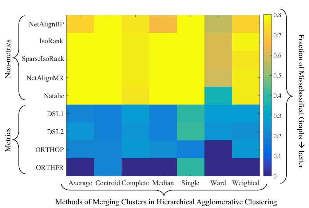
Figure 1: A clustering experiment using metrics and non-metrics (y-axis) for different clustering parameters (x-axis) is shown in (a), left. We sample graphs with $n=50$ nodes from the six classes, shown in the adjacent table in (d), bottom-center. We compute distances between them using nine different algorithms from Table 1. Only the distances in our family (DSL1, DSL2, ORTHOP, and ORTHFR) are metrics. The resulting graphs are clustered using hierarchical agglomerative clustering [28] using $Average$, $Centroid$, $Complete$, $Median$, $Single$, $Ward$, $Weighted$ as a means of merging clusters. Colors represent the fraction of misclassified graphs, with the minimal misclassification rate per distance labeled explicitly. Metrics outperform other distance scores across all clustering methods. The error rate of a random guess is $\approx 0.8$. Subfigures (b) and (c), top center and right, shows that non-metric distances produce triangle inequality violations (TIVs) which contribute to poor clustering results; the figure shows the fraction of TIVs within different $10$-node and $50$ node graph families under these algorithms. Finally, subfigure (e), bottom right, shows the fraction of triangle inequality violations for different algorithms on the small graphs dataset of all 7-node graphs.

We stress here that this result is non-obvious: is not true that adding any linear term to $d_{S}$ leads to a quantity that satisfies the triangle inequality. It is precisely because $D_{\psi_{A},\psi_{B}}$ contains pairwise distances that Theorem 4 holds. We can similarly extend Theorem 2:

Theorem 5.

If $S=\amsmathbb{W}^{n}$ and $\|\cdot\|$ is an arbitrary entry-wise norm, then $d_{S}$ given by (6) is a pseudometric over $\Omega=\amsmathbb{S}^{n}\times\Psi_{\tilde{\Omega}}^{n}$, the set of symmetric graphs embedded in $(\tilde{\Omega},\tilde{d})$. Moreover, if $\|\cdot\|$ is an arbitrary entry-wise or operator norm, then the symmetric extension $\bar{d}_{S}$ of (6) is a pseudometric over $\Omega=\amsmathbb{R}^{n\times n}\times\Psi_{\tilde{\Omega}}^{n}$.

Adding the linear term (5) in $d_{S}$ has significant practical advantages. Beyond expressing exogenous attributes, a linear term involving colors, combined with a Kronecker distance, translates into hard constraints: any permutation attaning a finite objective value must map nodes in one graph to nodes of the same color. Theorem 5 therefore implies that such constraints can thus be added to the optimization problem, while maintaining the metric property. In practice, as the number of variables in optimization problem (4) is $n^{2}$, incorporating such hard constraints can significantly reduce the problem’s computation time; we illustrate this in the next section. Note that adding (5) to $d_{\mathbb{O}^{n}}$ does not preserve the metric propery.

5 Experiments

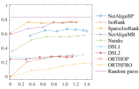
Figure 2: (a) Effect of introducing TIVs on the performance of different algorithms on the clustering experiment of Figure 1(a) when using the Ward method. (b) Cosine similarity between the Laplacian of distances produced by each algorithm and the one by EXACT. (c) Distance between nearest neighbor (NN) graphs induced by different algorithms and NN graph induced by EXACT.

Graphs. We use synthetic graphs from six classes summarized in the table in Fig. 1(d). In addition, we use a dataset of small graphs, comprising all $853$ connected graphs of $7$ nodes [46]. Finally, we use a collaboration graph with $5242$ nodes and $14496$ edges representing author collaborations [42].

(Non-metric) Distance Score Algorithms
NetAlignBP	Network Alignment using Belief Propagation [9, 34]
IsoRank	Neighborhood Topology Isomorphism using Page Rank [55, 34]
SparseIsoRank	Neighborhood Topology Sparse Isomorphism using Page Rank [9, 34]
InnerPerm	Inner Product Matching with Permutations [43]
InnerDSL1	Inner Product Matching with Matrices in $\amsmathbb{W}^{n}$ and entry-wise 1-norm [43]
InnerDSL2	Inner Product Matching with Matrices in $\amsmathbb{W}^{n}$ and Frobenius norm [43]
NetAlignMR	Iterative Matching Relaxation [35, 34]
Natalie (V2.0)	Improved Iterative Matching Relaxation [22, 21]
Metrics from our Family (4)
EXACT	Chemical Distance via brute force search over GPU
DSL1	Doubly Stochastic Chemical Distance $d_{\amsmathbb{W}^{n}}$ with entry-wise 1-norm
DSL2	Doubly Stochastic Chemical Distance $d_{\amsmathbb{W}^{n}}$ with Frobenius norm
ORTHOP	Orthogonal Relaxation of Chemical Distance $d_{\mathbb{O}^{n}}$ with operator 2-norm
ORTHFR	Orthogonal Relaxation of Chemical Distance $d_{\mathbb{O}^{n}}$ with Frobenius norm

Table 1: Competitor Distance Scores & Our Metrics

​$k$	​$\|P\|_{0}$	​$\|\!AP\!\!-\!\!PA\!\|_{0}$	$\tau$
​1	​3,747,960	​100.569	133s
​2	​239,048	​3,004	104s
​3	​182,474	​2,036	136s
​4	​182,016	​2,030	169s
​5	​182,006	​2,030	200s

Figure 3: (a) Effect of coloring/hard constraints on the numbers of variables ($\|P\|_{0}$) and terms of objective ($\|AP-PA\|_{0}$) using $k$ iterations of the WL coloring algorithm. The last column shows the execution time of WL on a 40 CPU machine using Apache Spark [63]. (b) Convergence of ADMM algorithm [14] computing DSL2 on two copies of the collaboration graph as a function of time, implemented using Apache Spark [63] on a 40 CPU machine.

Algorithms. We compare our metrics to several competitors outlined in Table 1 (see also Appendix E). All receive only two unlabeled undirected simple graphs $A$ and $B$ and output a matching a matrix $\hat{P}$ either in $\amsmathbb{W}^{n}$ or in $\mathbb{P}^{n}$ estimating $P^{*}$. If $\hat{P}\in\mathbb{P}^{n}$, we compute $\|A\hat{P}-\hat{P}B\|_{1}$. If $\hat{P}\in\amsmathbb{W}^{n}$, then we compute both $\|A\hat{P}-\hat{P}B\|_{1}$ and $\|A\hat{P}-\hat{P}B\|_{F}$; all norms are entry-wise. We also implement our two relaxations $d_{\amsmathbb{W}}$ and $d_{\mathbb{O}^{n}}$, for two different matrix norm combinations.

Clustering Graphs. The difference between our metrics and non-metrics is striking when clustering graphs. This is illustrated by the clustering experiment shown in Fig. 1(a). Graphs of size $n=50$ from the 6 classes in Fig. 1(d) are clustered together through hierarchical agglomerative clustering. We compute distances between them using nine different algorithms; only the distances in our family (DSL1, DSL2, ORTHOP, and ORTHFR) are metrics. The quality of clusters induced by our metrics are far superior than clusters induced by non-metrics; in fact, ORTHOP and ORTHFR can lead to no misclassifications. This experiment strongly suggests our produced metrics correctly capture the topology of the metric space between these larger graphs.

Triangle Inequality Violations (TIV). Given graphs $A$, $B$ and $C$ and a distance $d$, a TIV occurs when $d(A,C)>d(A,B)+d(B,C)$. Being metrics, none of our distances induce TIVs; this is not the case for the remaining algorithms in Table 1. Fig. 1(b) and (c) show the TIV fraction across the synthetic graphs of Fig. 1(d), while Fig. 1(e) shows the fraction of TIVs found on the $853$ small graphs ($n=7$). NetAlignMR also produces no TIVs on the small graphs, but it does induce TIVs in synthetic graphs. We observe that it is easier to find TIVs when graphs are close: in synthetic graphs, TIVs abound for $n=10$. No algorithm performs well across all categories of graphs.

Effect of TIVs on Clustering. Next, to investigate the effect of TIVs on clustering, we artificially introduced triangle inequality violations into the pairs of distances between graphs. We then re-evaluated clustering performance for hierarchical agglomerative clustering using the Ward method, which performed best in Fig. 1(a). Fig. 2(a) shows the fraction of misclassified graphs as the fraction of TIVs introduced increases. To incur as small a perturmbation on distances as possible, we introduce TIVs as follows: For every three graphs, $A,B,C$, with probability $p$, we set $d(A,C)=d(A,B)+d(B,C)$. Although this does not introduce a TIV w.r.t. $A$,$B$, and $C$, this distortion does introduce TIVs w.r.t. other triplets involving $A$ and $C$. We repeat this 20 times for each algorithm and each value of $p$, and compute the average fraction of TIVs, shown in the $x$-axis, and the average fraction of misclassified graphs, shown in the $y$-axis. As little as $1\%$ TIVs significantly deteriorate clustering performance. We also see that, even after introducing TIVs, clustering based on metrics outperforms clustering based on non-metrics.

Comparison to Chemical Distance. We compare how different distance scores relate to the chemical distance EXACT through two experiments on the small graphs (computation on larger graphs is prohibitive). In Figure 2(b), we compare the distances between small graphs with $7$ nodes produced by the different algorithms and EXACT using the DISTATIS method of [1]. Let $D\in\amsmathbb{R}_{+}^{835\times 835}$ be the matrix of distances between graphs under an algorithm. DISTATIS computes the normalized Laplacian of this matrix, given by $L=-UDU/\|UDU\|_{2}$ where $U=I-\frac{{\bf 1}{\bf 1}^{\top}}{n}$. The DISTATIS score is the cosine similarity of such Laplacians (vectorized). We see that our metrics produce distances attaining high similarity with EXACT, though NetAlignBP has the highest similarity. We measure proximity to EXACT with an additional test. Given $D$, we compute the nearest neighbor (NN) meta-graph by connecting a graph in $D$ to every graph at distance less than its average distance to other graps. This results in a (labeled) meta-graph, which we can compare to the NN meta-graph induced by other algorithms, measuring the fraction of distinct edges. Fig. 2(c) shows that our algorithms perform quite well, though Natalie yields the smallest distance to EXACT.

Incorporating Constraints. Computation costs can be reduced through metric embeddings, as in (6). To show this, we produce a copy of the $5242$ node collaboration graph with permuted node labels. We then run the WL algorithm (see Appendix D) to produce structural colors, which induce coloring constraints on $P\in\amsmathbb{W}^{n}$. The support of $P$ (i.e., the number of variables in the optimization (4)), the support of $AP-PA$ (i.e., the number of non-zero summation terms in the objective of (4)), as well as the execution time $\tau$ of the WL algorithm, are summarized in Fig. 3(b). The original unconstrained problem involves $5242^{2}\approx 27.4$M variables. However, after using WL and induced costraints, the effective dimension of the optimization problem (4) reduces considerably. This, in turn, speeds up convergence time, shown in Fig. 3(b): including the time to compute constraints, a solution is found 110 times faster after the introduction of the constraints.

6 Conclusion

Our work suggests that incorporating soft and hard constraints has a great potential to further improve the efficiency of our metrics. In future work, we intend to investigate and characterize the resulting equivalence classes under different soft and hard constraints and to quantify these gains in efficiency, especially in parallel implementations like ADMM. Determining the necessity of the conditions used in proving that $d_{S}$ is a metric is also an open problem.

Appendix A Proof of Lemmas 1–7

A.1 Proof of Lemma 1

Consider $P^{\prime}\in\mathop{\arg\,\min}_{P\in S}\|AP-PB\|$, and $P^{\prime\prime}\in\mathop{\arg\,\min}_{P\in S}\|BP-PC\|$. Then, from closure under multiplication, $P^{\prime}P^{\prime\prime}\in S$. Hence,

$$d_{S}(A,C) \leq\|AP^{\prime}P^{\prime\prime}-P^{\prime}P^{\prime\prime}C\|$$

$$\leq\|AP^{\prime}P^{\prime\prime}-P^{\prime}BP^{\prime\prime}\|+\|P^{\prime}BP^{\prime\prime}-P^{\prime}P^{\prime\prime}C\|$$

$$=\|(AP^{\prime}-P^{\prime}B)P^{\prime\prime}\|+\|P^{\prime}(BP^{\prime\prime}-P^{\prime\prime}C)\|$$

$$\leq\|AP^{\prime}-P^{\prime}B\|+\|BP^{\prime\prime}-P^{\prime\prime}C\|$$

where the last inequality follows from the fact that $P^{\prime},P^{\prime\prime}$ are contractions. $\square$

A.2 Proof of Lemma 2

Observe that property (b) implies that, for all $P\in S$, $P$ is invertible and $P^{-1}\in S$. Hence, $\|AP\!-\!PB\|\!=\!\|P(P^{-1}\!A\!-\!BP^{-1})P\|\!\leq\!\|BP^{-1}\!-\!P^{-1}A\|,$ as $P$ is a contraction w.r.t $\|\cdot\|$. We can similarly show that $\|BP^{-1}-P^{-1}A\|\leq\|AP-PB\|,$ hence $\|AP-PB\|=\|BP^{-1}-P^{-1}A\|.$ As $S$ is closed under inversion, $\min_{P\in S}f(P)=\min_{P:P^{-1}\in S}f(P)$, so $d_{S}(A,B)=\min_{P\in S}\|BP^{-1}-P^{-1}A\|=\min_{P:P^{-1}\in S}\|BP^{-1}-P^{-1}A\|=\min_{P\in S}\|BP-PA\|=d_{S}(B,A).$ $\square$

A.3 Proof of Lemma 3

If $I\in S$, then $0\leq d_{S}(A,A)\leq\|AI-IA\|=0$. $\square$

A.4 Proof of Lemma 4

Observe first that all vector $p$-norms are invariant to permutations a vector’s entries; hence, for any vector $x\in\amsmathbb{R}^{d}$, if $P\in\mathbb{P}^{n}$, $\|Px\|_{p}=\|x\|_{p}$. Hence, if $\|\cdot\|$ is an operator $p$-norm, $\|P\|=1,$ for all $P\in S.$ Every operator norm is submultiplicative; as a result $\|PA\|\leq\|P\|\|A\|=\|A\|$ and, similarly, $\|AP\|\leq\|A\|$, so the lemma follows for operator norms. On the other hand, if $\|\cdot\|$ is an entry-wise norm, then $\|A\|$ is invariant to permutations of either $A$’s rows or columns. Matrices $PA$ and $AP$ precisely amount to such permutations, so $\|PA\|=\|AP\|=\|A\|$ and the lemma follows also for entrywise norms. $\square$

A.5 Proof of Lemma 5

Any $U\in\mathbb{O}^{n}$ is an orthogonal matrix; hence, $\|U\|_{2}=\|U\|_{F}=1$. Both norms are submultiplicative: the first as an operator norm, the second from the Cauchy-Schwartz inequality. Hence, for $U\in\mathbb{O}^{n}$, we have $\|UA\|\leq\|U\|\|A\|=\|A\|.$ $\square$

A.6 Proof of Lemma 6

By the Birkoff-con Neumann theorem [11], $\amsmathbb{W}^{n}=\mathtt{conv}(\mathbb{P}^{n})$. Hence, for any $W\in\amsmathbb{W}^{n}$ there exist $P_{i}\in\mathbb{P}^{n}$, $\theta_{i}>0$, $i=1,\ldots,k$, such that $W=\sum_{i=1}^{k}\theta_{i}P_{i}$ and $\sum_{i=1}^{k}\theta_{i}=1.$ Both operator and entrywise $p$-norms are convex functions; hence, by Jensen’s inequality, for any $A\in\amsmathbb{R}^{n\times N}$: $\|WA\|\leq\textstyle\sum_{i=1}^{k}\theta_{i}\|P_{i}A\|\leq\textstyle\sum_{i=1}^{k}\theta_{i}\|A\|=\|A\|$ where the last ineqality follows by Lemma 4. The statement $\|AW\|\leq\|A\|$ follows similarly. $\square$

A.7 Proof of Lemma 7

By transpose invariance and the symmetry of $A$ and $B$, we have that: $\|AP-PB\|=\|BP^{\top}-P^{\top}A\|.$ Moreover, as $S$ is closed under transposition, $\min_{P\in S}f(P)=\min_{P^{\top}\in S}f(P)$. Hence, $d_{S}(A,B)=\min_{P\in S}\|BP^{\top}-P^{\top}A\|=\min_{P^{\top}\in S}\|BP^{\top}-P^{\top}A\|=d_{S}(B,A).$ $\square$

Appendix B Proof of Theorems 4 and 5

We begin by establishing conditions under which $d_{S}$ satisfies the triangle inequality (3d). We note that, in contrast to Lemma 1, we require the additional condition that $S\subseteq\amsmathbb{W}^{n}$, which is not satisfied by $\mathbb{O}^{n}$.

Lemma 8.

Given a norm $\|\cdot\|$, suppose that $S$ is (a) contractive w.r.t. $\|\cdot\|$, (b) closed under multiplication, and (c) is a subset of $\amsmathbb{W}^{n}$, i.e., contains only doubly stochastic matrices. Then, for any $(A,\psi_{A}),(B,\psi_{B}),(C,\psi_{C})$ in $\amsmathbb{R}^{n\times n}\times\Psi_{\tilde{\Omega}}$, $d_{S}((A,\psi_{A}),(C,\psi_{B}))\leq d_{S}((A,\psi_{A}),(B,\psi_{B}))+d_{S}((B,\psi_{B}),(C,\psi_{C})).$

Proof.

Consider

$$P^{\prime}\in\mathop{\arg\,\min}_{P\in S}\left(\|AP-PB\|+\mathop{\mathsf{tr}}\left(P^{\top}D_{\psi_{A},\psi_{B}}\right)\right),$$

and

$$P^{\prime\prime}\in\mathop{\arg\,\min}_{P\in S}\left(\|BP-PC\|+\mathop{\mathsf{tr}}\left(P^{\top}D_{\psi_{B},\psi_{C}}\right)\right).$$

Then, from closure under multiplication, $P^{\prime}P^{\prime\prime}\in S$. We have that

$$\begin{split}d_{S}((A,\psi_{A}),(C,\psi_{C}))\leq\|AP^{\prime}P^{\prime\prime}-P^{\prime}P^{\prime\prime}C\|\\ +\mathop{\mathsf{tr}}\left[(P^{\prime}P^{\prime\prime})^{\top}D_{\psi_{A}\psi_{C}}\right]\end{split}$$

As in the proof of Lemma 1, we can show that

$$\|AP^{\prime}P^{\prime\prime}-P^{\prime}P^{\prime\prime}C\| \leq\|AP^{\prime}-P^{\prime}B\|+\|BP^{\prime\prime}-P^{\prime\prime}C\|$$

using the fact that both $P^{\prime}$ and $P^{\prime\prime}$ are contractions, while

$$\mathop{\mathsf{tr}}\big{[}(P^{\prime} P^{\prime\prime})^{\top}D_{\psi_{A}\psi_{C}}\big{]}=$$

$$=\sum_{u,v\in[n]}\sum_{k\in[n]}\left(P^{\prime}_{uk}P^{\prime\prime}_{kv}\tilde{d}(\psi_{A}(u),\psi_{C}(v)))\right)$$

$$\leq\sum_{u,v\in[n]}\sum_{k\in[n]}\big{[}P^{\prime}_{uk}P^{\prime\prime}_{kv}\big{(}\tilde{d}(\psi_{A}(u),\psi_{B}(k))$$

$$\qquad+\tilde{d}(\psi_{B}(k),\psi_{C}(v))\big{)}\big{]}$$

$$\text{ (as }\tilde{d}\text{ is a metric, and}P^{\prime},P^{\prime\prime}\text{are non-negative) }$$

$$=\sum_{u,k\in[n]}P^{\prime}_{uk}\ \tilde{d}(\psi_{A}(u),\psi_{B}(k))\sum_{v\in[n]}P^{\prime\prime}_{kv}$$

$$\quad+\sum_{k,v\in[n]}P^{\prime\prime}_{kv}\tilde{d}(\psi_{B}(k),\psi_{C}(v))\sum_{u\in[n]}P^{\prime}_{uk}$$

$$\leq\mathop{\mathsf{tr}}\left((P^{\prime})^{\top}D_{\psi_{A},\psi_{B}}\right)+\mathop{\mathsf{tr}}\left((P^{\prime\prime})^{\top}D_{\psi_{B},\psi_{C}}\right),$$

where the last inequality follows as both $P,P^{\top}$ are $\|\cdot\|_{1}$-norm bounded by 1 for every $P\in S$. ∎

The weak property (3e) is again satisfied provided the identity is included in $S$.

Lemma 9.

If $I\in S$, then $d_{S}((A,\psi_{A}),(A,\psi_{A}))=0$ for all $A\in\amsmathbb{R}^{n\times n}$.

Proof.

Indeed, $0\leq d_{S}((A,\psi_{A},(A,\psi_{A}))\leq\|AI-IA\|+\sum_{u\in[n]}\tilde{d}(\psi_{A}(u),\psi_{A}(u))=0$. ∎

To attain symmetry over $\Omega=\amsmathbb{R}^{n\times n}$, we again rely on closure under inversion, as in Lemma 10; nonetheless, in contrast to Lemma 10, due to the linear term, we also need to assume orthogonality of $S$.

Lemma 10.

Given a norm $\|\cdot\|$, suppose that $S$ (a) is contractive w.r.t. $\|\cdot\|$, (b) is closed under inversion, and (c) is a subset of $\mathbb{O}^{n}$, i.e., contains only orthogonal matrices. Then, $d_{S}((A,\psi_{A}),(B,\psi_{B}))=d_{S}((B,\psi_{B}),(A,\psi_{A}))$ for all $(A,\psi_{A}),(B,\psi_{B})\in\amsmathbb{R}^{n\times n}\times\Psi_{\tilde{\Omega}}$.

Proof.

As in the proof of Lemma 2, we can show that contractiveness w.r.t. $\|\cdot\|$ along with closure under inversion imply that: $\|AP-PB\|=\|BP^{-1}-P^{-1}A\|.$ As $S$ is closed under inversion, $\min_{P\in S}f(P)=\min_{P:P^{-1}\in S}f(P)$ for all $f:S\to\amsmathbb{R}$, while orthogonality implies $P^{-1}=P^{\top}$ for all $P\in S$. Hence, $d_{S}((A,\psi_{A}),(B,\psi_{B}))$ equals:

$$\min_{P\in S} \left[\|AP-PB\|+\mathop{\mathsf{tr}}\left(P^{\top}D_{\psi_{A},\psi_{B}}\right)\right]$$

$$=\min_{P\in S}\left[\|BP^{-1}-P^{-1}A\|+\mathop{\mathsf{tr}}\left(P^{-1}D_{\psi_{A},\psi_{B}}\right)\right]$$

$$=\min_{P\in S}\left[\|BP^{-1}-P^{-1}A\|+\mathop{\mathsf{tr}}\left(\left(P^{-1}\right)^{\top}D_{\psi_{A},\psi_{B}}^{\top}\right)\right]$$

$$=\min_{P^{-1}\in S}\left[\|BP^{-1}-P^{-1}A\|+\mathop{\mathsf{tr}}\left(\left(P^{-1}\right)^{\top}D_{\psi_{A},\psi_{B}}^{\top}\right)\right]$$

$$=d_{S}((B,\psi_{B}),(A,\psi_{A})).\qquad\qquad\qquad\qquad\qquad\qed$$

Theorem 4 therefore follows from the above lemmas, as $S=\mathbb{P}^{n}$ contains $I$, it is closed under multiplication and inversion, is a subset of $\amsmathbb{W}^{n}\cap\mathbb{O}^{n}$, and is contractive w.r.t. all operator and entrywise norms. Theorem 5 also follows by using the following lemma, along with Lemmas 8 and 9.

Lemma 11.

Suppose that $\|\cdot\|$ is transpose invariant, and $S$ is closed under transposition. Then, $d_{S}((A,\psi_{A}),(B,\psi_{B}))=d_{S}((B,\psi_{B}),(A,\psi_{A}))$ for all $(A,\psi_{A}),(B,\psi_{B})\in\amsmathbb{S}^{n}\times\Psi_{\tilde{\Omega}}$.

Proof.

By transpose invariance of $\|\cdot\|$ and the symmetry of $A$ and $B$, we have that: $\|AP-PB\|=\|BP^{\top}-P^{\top}A\|.$ Moreover, as $S$ is closed under transposition, $\min_{P\in S}f(P)=\min_{P^{\top}\in S}f(P)$ for any $f:S\to\amsmathbb{R}$. Hence, $d_{S}((A,\psi_{A}),(B,\psi_{B}))$ equals

$$\min_{P\in S} \left[\|AP-PB\|+\mathop{\mathsf{tr}}\left(P^{\top}D_{\psi_{A},\psi_{B}}\right)\right]$$

$$=\min_{P\in S}\left[\|BP^{\top}-P^{\top}A\|+\mathop{\mathsf{tr}}\left(PD_{\psi_{A},\psi_{B}}^{\top}\right)\right]$$

$$=\min_{P^{\top}\in S}\|BP^{\top}-P^{\top}A\|+\mathop{\mathsf{tr}}\left((P^{\top})^{\top}D_{\psi_{B},\psi_{A}}\right)$$

$$=d_{S}((B,\psi_{B}),(A,\psi_{A})).\qquad\qquad\qquad\qquad\qquad\qed$$

Appendix C Metric Computation Over the Stiefler Manifold.

In this section, we describe how to compute the metric $d_{S}$ in polynomial time when $S=\mathbb{O}^{n}$ and $\|\cdot\|$ is the Frobenious norm or the operator 2-norm. The algorithm for the Frobenius norm, and the proof of its correctness, is due to [57]; we include it in this appendix for completeness, along with its extension to the operator norm.

Both cases make use of the following lemma:

Lemma 12.

For any matrix $M\in\amsmathbb{R}^{n\times n}$ and any matrix $P\in\mathbb{O}^{n}$ we have that $\|PM\|=\|MP\|=\|M\|$, where $\|\cdot\|$ is either the Frobenius or operator 2-norm.

Proof.

Recall that the operator 2-norm $\|\cdot\|_{2}$ is $\|M\|_{2}=\sup_{x\neq 0}{\|Mx\|_{2}/\|x\|_{2}}=\sqrt{\sigma_{\max}(M^{\top}M)}=\sqrt{\sigma_{\max}(MM^{\top})}=\|M^{\top}\|_{2}.$ where $\sigma_{\max}$ denotes the largest singular value. Hence, $\|PM\|_{2}=\sup_{x\neq 0}{\|PMx\|_{2}/\|x\|_{2}}=\sqrt{\sigma_{\max}(M^{\top}P^{\top}PM)}=\sqrt{\sigma_{\max}(M^{\top}M)}=\|M\|_{2}.$ as $P^{\top}P=I$. Using the fact that $\|M\|_{2}=\|M^{\top}\|_{2}$ for all $M\in\amsmathbb{R}^{n\times n}$, as well as that $PP^{\top}=I$, we can show that $\|MP\|_{2}=\|P^{\top}M^{\top}\|_{2}=\|M^{\top}\|_{2}=\|M\|_{2}$.

The Frobenius norm is $\|M\|_{F}=\sqrt{\mathop{\mathsf{tr}}(M^{\top}M)}=\sqrt{\mathop{\mathsf{tr}}(MM^{\top})}=\|M^{\top}\|_{F},$ hence $\|PM\|_{F}=\sqrt{\mathop{\mathsf{tr}}(M^{\top}P^{\top}PM)}=\sqrt{\mathop{\mathsf{tr}}(M^{\top}M)}=\|M\|_{F}$ and, as in the case of the operator norm, we can similarly show $\|MP\|_{F}=\|P^{\top}M^{\top}\|_{F}=\|M^{\top}\|_{F}=\|M\|_{F}$. ∎

In both norm cases, for $A,B\in\amsmathbb{S}^{n}$, we can compute $d_{S}$ using a simple spectral decomposition. Let $A=U\Sigma_{A}U^{T}$ and $B=V\Sigma_{B}V^{T}$ be the spectral decomposition of $A$ and $B$. As $A$ and $B$ are real and symmetric, we can assume $U,V\in\mathbb{O}^{n}$. Recall that $U^{-1}=U^{\top}$ and $V^{-1}=V^{\top}$, while $\Sigma_{A}$ and $\Sigma_{B}$ are diagonal and contain the eigenvalues of $A$ and $B$ sorted in increasing order; this orderning matters for computations below.

The following theorem establishes that this decomposition readily yields the distance $d_{S}$, as well as the optimal orthogonal matrix $P^{*}$, when $\|\cdot\|=\|\cdot\|_{F}$:

Theorem 6 ([57]).

$d_{S}(A,B)\triangleq\min_{P\in S}\|AP-PB\|_{F}=\|\Sigma_{A}-\Sigma_{B}\|_{F}$ and the minimum is attained by $P^{*}=UV^{\top}$.

Proof.

The proof makes use of the following lemma by [30].

Lemma 13.

If $A$ and $B$ are Hermitian matrices with eigenvalues $a_{1}\leq a_{2}\leq...\leq a_{n}$ and $b_{1}\leq b_{2}\leq...\leq b_{n}$ then

$$\|A-B\|^{2}_{F}\geq{\sum^{n}_{i=1}(a_{i}-b_{i})^{2}}$$ (7)

Remark 1.

Note that if $\Sigma_{A}$ and $\Sigma_{B}$ are diagonal matrices with the ordered eigenvalues of $A$ and $B$ in the diagonal, then Lemma 13 can be written as $\|A-B\|_{F}\geq\|\Sigma_{A}-\Sigma_{B}\|_{F}$.

For any $P\in\mathbb{O}^{n}$ and $\|\cdot\|=\|\cdot\|_{F}$ we have

$$\|AP-PB\| =\|(A-PBP^{-1})P\|\stackrel{{\scriptstyle\text{Lem.}~{}\ref{eqlemma}}}{{=}}\|A-PBP^{\top}\|$$

$$=\|U\Sigma_{A}U^{\top}-PV\Sigma_{B}V^{\top}P^{\top}\|$$

$$=\|U(\Sigma_{A}-U^{\top}PV\Sigma_{B}V^{\top}P^{\top}U)U^{\top}\|$$

$$\stackrel{{\scriptstyle\text{Lem.}~{}\ref{eqlemma}}}{{=}}\|\Sigma_{A}-U^{\top}PV\Sigma_{B}V^{\top}P^{\top}U\|$$

$$=\|\Sigma_{A}-\Delta\Sigma_{B}\Delta^{\top}\|$$

where we define $\Delta\triangleq U^{\top}PV$. As a product of orthogonal matrices, $\Delta\in\mathbb{O}^{n}$. Notice that

$$\|\Sigma_{A}-\Delta\Sigma_{B} \Delta^{\top}\|=$$

$$=\|\Sigma_{A}-\Delta\Sigma_{A}\Delta^{\top}+\Delta(\Sigma_{B}-\Sigma_{A})\Delta^{\top}\|$$

$$\leq\|\Sigma_{A}-\Delta\Sigma_{A}\Delta^{\top}\|+\|\Delta(\Sigma_{B}-\Sigma_{A})\Delta^{\top}\|$$

$$\stackrel{{\scriptstyle\text{Lem.}~{}\ref{eqlemma}}}{{=}}\|\Sigma_{A}-\Delta\Sigma_{A}\Delta^{\top}\|+\|\Sigma_{B}-\Sigma_{A}\|.$$

Therefore, for any $P\in\mathbb{O}^{n}$, $\|\Sigma_{A}-\Sigma_{B}\|\leq d_{S}(A,B)\leq\|\Sigma_{A}-\Delta\Sigma_{A}\Delta^{\top}\|+\|\Sigma_{B}-\Sigma_{A}\|,$ where the first inequality follows by Lemma 13 if we notice that $\|AP-PB\|=\|A-PBP^{-1}\|$ and that $PBP^{-1}$ and $B$ have the same spectrum for any $P$. If we choose $P=UV^{\top}$ then $\Delta=I$ and the result follows. ∎

We can compute $d_{S}$ when $S=\mathbb{O}^{n}$ and $\|\cdot\|$ is the operator norm in the exact same way.

Theorem 7.

Let $\|\cdot\|=\|\cdot\|_{2}$ be the operator 2-norm. Then, $d_{S}(A,B)\triangleq\min_{P\in S}\|AP-PB\|_{2}=\|\Sigma_{A}-\Sigma_{B}\|_{2}$ and the minimum is attained by $P^{*}=UV^{\top}$.

Proof.

The proof follows the same steps as the proof of Theorem 6, using Lemma 14 below instead of Lemma 13.

Lemma 14.

If $A$ and $B$ are Hermitian matrices with eigenvalues $a_{1}\leq a_{2}\leq...\leq a_{n}$ and $b_{1}\leq b_{2}\leq...\leq b_{n}$ then

$$\|A-B\|_{2}\geq\max_{i}|a_{i}-b_{i}|.$$ (8)

Remark 2.

Note that if $\Sigma_{A}$ and $\Sigma_{B}$ are diagonal matrices with the ordered eigenvalues of $A$ and $B$ in the diagonal, then Lemma 14 can be written as $\|A-B\|_{2}\geq\|\Sigma_{A}-\Sigma_{B}\|_{2}$.

Proof of Lemma 14.

Let $\tilde{B}=-B$ have eigenvalues $\tilde{b}_{1}\leq\tilde{b}_{2}\leq...\leq\tilde{b}_{n}$ and let $C=A+\tilde{B}$ have eigenvalues $c_{1}\leq c_{2}\leq...\leq c_{n}$. We make use of the following lemma by Weyl [31] to lower bound $c_{n}$.

Lemma 15.

If $X$ and $Y$ are Hermitian with eigenvalues $x_{1}\leq...\leq x_{n}$ and $y_{1}\leq...\leq y_{n}$ and if $X+Y$ has eigenvalues $w_{1}\leq...\leq w_{n}$ then $x_{i-j+1}+y_{j}\leq w_{i}$ for all $i=1,\ldots,n$ and $j=1,\ldots,i$.

If we choose $X=\tilde{B}$, $Y=A$ and $i=n$ we get $a_{j}+\tilde{b}_{n+1-j}\leq c_{n}$ for all $j=1,\ldots,n$.

Since $\tilde{b}_{n+1-j}=-{b}_{j}$ we get that $a_{j}-{b}_{j}\leq c_{n}$, for any $j$. Similarly, by exchanging the role of $A$ and $B$, we can lower bound the largest eigenvalue of $B-A$, say $d_{n}$, by $b_{j}-a_{j}$ for any $j$. Notice that, by definition of the operator norm and the fact that $A-B$ is Hermitian, $\|A-B\|_{2}\geq|c_{n}|$ and $\|B-A\|_{2}\geq|d_{n}|$. Since $\|B-A\|_{2}=\|A-B\|_{2}$ we have that $\|A-B\|_{2}\geq\max\{|c_{n}|,|d_{n}|\}\geq\max\{c_{n},d_{n}\}\geq\max\{a_{j}-b_{j},b_{j}-a_{j}\}=|a_{j}-b_{j}|$ for all $j$. Taking the maximum over $j$ we get that $\|A-B\|_{2}\geq\max_{j}|a_{j}-b_{j}|$, and the lemma follows. ∎

The proof of Thm. 7 proceeds along the same steps as the above proof, using again the fact that, by Lemma 12, $\|M\|_{2}=\|MP\|_{2}=\|PM\|_{2}$ for any $P\in\mathbb{O}^{n}$ and any matrix $M$, along with Lemma 15. ∎

Appendix D The Weisfeiler-Lehman (WL) Algorithm.

The WL algorithm [60] is a graph isomorphism heuristic. To gain some intuition on the algorithm, note that two isomorphic graphs must have the same degree distribution. More broadly, the distributions of $k$-hop neighborhoods in the two graphs must also be identical. Building on this, to test if two undirected, unweighted graphs are isomorphic, WL colors the nodes of a graph $G(V,E)$ iteratively. At iteration $0$, each node $v\in V$ receives the same color $c^{0}(v):=1$. Colors at iteration $k+1\in\amsmathbb{N}$ are defined recursively via $c^{k+1}(v):=\mathsf{hash}\left(\mathsf{sort}\left(\textsf{clist}^{k}_{v}\right)\right)$where $\mathsf{hash}$ is a perfect hash function, and $\textsf{clist}^{k}_{v}=[c^{k}(u):(u,v)\in E)]$ is a list containing the colors of all of $v$’s neighbors at iteration $k$. Intuitively, two nodes in $V$ share the same color after $k$ iterations if their $k$-hop neighborhoods are isomorphic. WL terminates when the partition of $V$ induced by colors is stable from one iteration to the next. This coloring extends to weighted directed graphs by appending weights and directions to colors in $\textsf{clist}_{v}^{k}$. After coloring two graphs $G_{A},G_{B}$, WL declares a non-isomorphism if their color distributions differ. If not, then they may be isomorphic and WL gives a set of constraints on candidate isomorphisms: a permutation $P$ under which $AP=PB$ must map nodes in $G_{A}$ to nodes in $G_{B}$ of the same color.

Appendix E Algorithms and Implementation Details

We outline here additional impementation details about the algorithms summarized in Table 1.

• NetAlignBP, IsoRank, SparseIsoRank and NetAlignMR, for which code is publicly available [34], are described by [9]. Natalie is described in [22]; code is again available [21]. All five algorithms output $P\in\mathbb{P}^{n}$.

• The algorithm in [43] outputs one $P\in\mathbb{P}^{n}$ and one $P^{\prime}\in\amsmathbb{W}^{n}$. We use $P\in\mathbb{P}^{n}$ to compute $\|AP-PB\|_{1}$ and call this InnerPerm. We use $P^{\prime}\in\amsmathbb{W}^{n}$ to compute $\|AP^{\prime}-P^{\prime}B\|_{1}$ and $\|AP^{\prime}-P^{\prime}B\|_{2}$ and call these algorithms InnerDSL1 and InnerDSL2 respectively. We use our own CVX-based projected gradient descent solver for the non-convex optimization problem the authors propose.

• DSL1 and DSL2 denote $d_{S}(A,B)$ when $S\in\amsmathbb{W}^{n}$ and $\|\cdot\|$ is $\|\cdot\|_{1}$ (element-wise) and $\|\cdot\|_{F}$, respectively. We implement them in Matlab (using CVX) as well as in C, aimed for medium size graphs and multi-core use. We also implemented a distributed version in Apache Spark [63] that scales to very large graphs over multiple machines based on the Alternating Directions Method of Multipliers [14].

• ORTHOP and ORTHFR denote $d_{S}(A,B)$ when $S\in\mathbb{O}^{n}$ and $\|\cdot\|$ is $\|\cdot\|_{2}$ (operator norm) and $\|\cdot\|_{F}$ respectively. We compute them using an eigendecomposition (See Appendix C).

• For small graphs, we compute $d_{\mathbb{P}^{n}}(A,B)$ using our brute-force GPU-based code. For a single pair of graphs with $n\geq 15$ nodes, EXACT already takes several days to finish. For $\|\cdot\|=\|\cdot\|_{1}$ in $d_{S}$ (element-wise or matrix norm), we have implemented the chemical distance as an integer value LP and solved it using branch-and-cut. It did not scale well for $n\geq 15$.

• We implemented the WL algorithm over Spark to run, multithreaded, on a machine with 40 CPUs.

We use all public algorithms as black boxes with their default parameters, as provided by the authors.

Appendix F Graphs of Different Sizes

For simplicity, we described our framework for graphs of equal sizes. However, we can extended in different ways to produce a metric for graphs of different sizes. These extensions all start by extending two graphs, $G_{A}$ and $G_{B}$, with dummy nodes such that the new graphs $G^{\prime}_{A}$ and $G^{\prime}_{B}$ have the same number of nodes. If $G_{A}$ has $n_{A}$ nodes and $G_{B}$ has $n_{B}$ nodes we can, for example, add $n_{B}$ dummy nodes to $G_{A}$ and $n_{A}$ dummy nodes to $G_{A}$. Once we have $G^{\prime}_{A}$ and $G^{\prime}_{B}$ of equal size, we can use the methods we already described to compute a distance between $G^{\prime}_{A}$ and $G^{\prime}_{B}$ and return this distance as the distance between $G_{A}$ and $G_{B}$.

The different ways of extending the graphs differ in how the dummy nodes connect to existing graph nodes, how dummy nodes connect to themselves, and what kind of penalty we introduce for associating dummy nodes with existing graph nodes. Method 1: One way of extending the graphs is to add dummy nodes and leave them isolated, i.e., with no edges to either existing nodes or other dummy nodes. Although this might work when both graphs are dense, it might lead to non desirable results when one of the graphs is sparse. For example, let $G_{A}$ be $3$ isolated nodes and $G_{B}$ be the complete graph on $4$ nodes minus the edges forming triangle $\{(1,2),(2,3),(3,1)\}$. Let us assume that $S=\mathbb{P}^{n}$, such that, when we compute the distance between $G_{A}$ and $G_{B}$, we produce an alignment between the graphs. One desirable outcome would be for $G_{A}$ to be aligned with the three nodes in $G_{B}$ that have no edges among them. This is basically solving the problem of finding a sparse subgraph inside a dense graph. However, computing $d_{S}(A^{\prime},B^{\prime})$, where $A^{\prime}$ and $B^{\prime}$ are the extended adjacency matrices, could equally well align $G_{A}$ with the $3$ dummy node of $G^{\prime}_{B}$. Method 2: Add dummy nodes and connect each dummy node to all existing nodes and all other dummy nodes. This avoids the issue described for method 1 but creates a similar non desirable situation: since the dummy nodes in each extended graph form a click, we might align $G_{A}$, or $G_{B}$, with just dummy nodes, instead of producing an alignment between existing nodes in $G_{A}$ and existing nodes in $G_{B}$. Method 3: If both $G_{A}$ and $G_{B}$ are unweighted graphs, a method that avoids both issues above (aligning a sparse graph with isolated dummy nodes or aligning a dense graphs with clicks of dummy nodes) is to connect each dummy node to all existing nodes and all other dummy nodes with edges of weight $1/2$. This method works because, when $S=\mathbb{P}^{n}$, it discourages alignments of pairs existing-existing nodes in $G_{A}$ with pairs dummy-dummy nodes or pairs dummy-existing nodes in $G_{B}$, and vice versa. Method 4: One can also discourage aligning existing node with dummy nodes by introducing a linear term as in (6).

References

- Abdi et al. [2005] H Abdi, A J O’Toole, D Valentin, and B Edelman. DISTATIS: The analysis of multiple distance matrices. In CVPR Workshops, 2005.
- Absil et al. [2009] P-A Absil, R Mahony, and R Sepulchre. Optimization algorithms on matrix manifolds. Princeton University Press, 2009.
- Ackermann et al. [2010] M R Ackermann, J Blömer, and C Sohler. Clustering for metric and nonmetric distance measures. ACM Transactions on Algorithms (TALG), 6(4):59, 2010.
- Aflalo et al. [2015] Y Aflalo, A Bronstein, and R Kimmel. On convex relaxation of graph isomorphism. PNAS, 112(10):2942–2947, 2015.
- Albert and Barabási [2002] R Albert and A-L Barabási. Statistical mechanics of complex networks. Reviews of Modern Physics, 74(1):47, 2002.
- Allen [2002] F H Allen. The Cambridge Structural Database: a quarter of a million crystal structures and rising. Acta Crystallographica Section B: Structural Science, 58(3):380–388, 2002.
- Angiulli and Pizzuti [2002] F Angiulli and C Pizzuti. Fast outlier detection in high dimensional spaces. In PKDD, 2002.
- Babai [2016] L Babai. Graph isomorphism in quasipolynomial time [extended abstract]. In STOC, 2016.
- Bayati et al. [2009] M Bayati, M Gerritsen, D F Gleich, A Saberi, and Y Wang. Algorithms for large, sparse network alignment problems. In ICDM, 2009.
- Beygelzimer et al. [2006] A Beygelzimer, S Kakade, and J Langford. Cover trees for nearest neighbor. In ICML, 2006.
- Birkhoff [1946] G Birkhoff. Three observations on linear algebra. Univ. Nac. Tucumán. Revista A, 5:147–151, 1946.
- Bollobás [1998] B Bollobás. Random graphs. In Modern Graph Theory, pages 215–252. Springer, 1998.
- Boyd and Vandenberghe [2004] S Boyd and L Vandenberghe. Convex Optimization. Cambridge university press, 2004.
- Boyd et al. [2011] S Boyd, N Parikh, E Chu, B Peleato, and J Eckstein. Distributed optimization and statistical learning via the alternating direction method of multipliers. Foundations and Trends® in Machine Learning, 3(1):1–122, 2011.
- Bunke [1997] H Bunke. On a relation between graph edit distance and maximum common subgraph. Pattern Recognition Letters, 18(8):689–694, 1997.
- Bunke and Shearer [1998] H Bunke and K Shearer. A graph distance metric based on the maximal common subgraph. Pattern Recognition Letters, 19(3):255–259, 1998.
- Chartrand et al. [1998] G Chartrand, G Kubicki, and M Schultz. Graph similarity and distance in graphs. Aequationes Mathematicae, 55(1-2):129–145, 1998.
- Clarkson [1999] K L Clarkson. Nearest neighbor queries in metric spaces. Discrete & Computational Geometry, 22(1):63–93, 1999.
- Clarkson [2006] K L Clarkson. Nearest-neighbor searching and metric space dimensions. Nearest-Neighbor Methods for Learning and Vision: Theory and Practice, pages 15–59, 2006.
- Conte et al. [2004] D Conte, P Foggia, C Sansone, and M Vento. Thirty years of graph matching in pattern recognition. International Journal of Pattern Recognition and Artificial Intelligence, 18(03):265–298, 2004.
- [21] M El-Kebir, J Heringa, and G Klau. Natalie, a tool for pairwise global network alignment. http://www.mi.fu-berlin.de/w/LiSA/Natalie.
- El-Kebir et al. [2015] M El-Kebir, J Heringa, and G W Klau. Natalie 2.0: Sparse global network alignment as a special case of quadratic assignment. Algorithms, 8(4):1035–1051, 2015.
- Elghawalby and Hancock [2008] H Elghawalby and E R Hancock. Measuring graph similarity using spectral geometry. In ICIAR, 2008.
- Erdös and Rényi [1959] P Erdös and A Rényi. On random graphs, i. Publicationes Mathematicae (Debrecen), 6:290–297, 1959.
- Fankhauser et al. [2011] S Fankhauser, K Riesen, and H Bunke. Speeding up graph edit distance computation through fast bipartite matching. In GBR, 2011.
- Ferrer et al. [2010] M Ferrer, E Valveny, F Serratosa, K Riesen, and H Bunke. Generalized median graph computation by means of graph embedding in vector spaces. Pattern Recognition, 43(4):1642–1655, 2010.
- Garey and Johnson [2002] M R Garey and D S Johnson. Computers and Intractability, volume 29. WH Freeman New York, 2002.
- Hartigan [1975] J A Hartigan. Clustering algorithms. Wiley New York, 1975.
- He et al. [2006] L He, C Y Han, and W G Wee. Object recognition and recovery by skeleton graph matching. In ICME, 2006.
- Hoffman and Wielandt [1953] A J Hoffman and H W Wielandt. The variation of the spectrum of a normal matrix. Duke Math. J, 20(1):37–39, 1953.
- Horn and Johnson [2012] R A Horn and C R Johnson. Matrix Analysis. Cambridge University Press, 2012.
- Indyk [1999] P Indyk. Sublinear time algorithms for metric space problems. In Proceedings of the thirty-first annual ACM symposium on Theory of computing, pages 428–434. ACM, 1999.
- Jain [2016] B J Jain. On the geometry of graph spaces. Discrete Applied Mathematics, 214:126–144, 2016.
- [34] A Khan, D Gleich, M Halappanavar, and A Pothen. Multicore codes for network alignment. https://www.cs.purdue.edu/homes/dgleich/codes/netalignmc/.
- Klau [2009] G W Klau. A new graph-based method for pairwise global network alignment. BMC bioinformatics, 10(1):S59, 2009.
- Kleinberg [2000] J Kleinberg. The small-world phenomenon: An algorithmic perspective. In STOC, 2000.
- Koca et al. [2012] J Koca, M Kratochvil, V Kvasnicka, L Matyska, and J Pospichal. Synthon model of organic chemistry and synthesis design, volume 51. Springer Science & Business Media, 2012.
- Koutra et al. [2013a] D Koutra, H Tong, and D Lubensky. Big-align: Fast bipartite graph alignment. In ICDM, 2013a.
- Koutra et al. [2013b] D Koutra, J T Vogelstein, and C Faloutsos. Deltacon: A principled massive-graph similarity function. In SDM, 2013b.
- Kuhn [1955] H W Kuhn. The hungarian method for the assignment problem. Naval Research Logistics Quarterly, 2(1-2):83–97, 1955.
- Kvasnička et al. [1991] V Kvasnička, J Pospíchal, and V Baláž. Reaction and chemical distances and reaction graphs. Theoretical Chemistry Accounts: Theory, Computation, and Modeling (Theoretica Chimica Acta), 79(1):65–79, 1991.
- [42] J Leskovec, J Kleinberg, and C Faloutsos. Stanford large network dataset collection. http://snap.stanford.edu/data/ca-GrQc.html.
- Lyzinski et al. [2016] V Lyzinski, D E Fishkind, M Fiori, J T Vogelstein, C E Priebe, and Guillermo Sapiro. Graph matching: Relax at your own risk. IEEE Transactions on Pattern Analysis and Machine Intelligence, 38(1):60–73, 2016.
- Macindoe and Richards [2010] O Macindoe and W Richards. Graph comparison using fine structure analysis. In SocialCom, 2010.
- Mahmoud et al. [1993] H M Mahmoud, R T Smythe, and J Szymański. On the structure of random plane-oriented recursive trees and their branches. Random Structures & Algorithms, 4(2):151–176, 1993.
- [46] B McKay. List of 7 node connected graphs. http://users.cecs.anu.edu.au/~bdm/data/graphs.html.
- Papadimitriou et al. [2010] P Papadimitriou, A Dasdan, and H Garcia-Molina. Web graph similarity for anomaly detection. Journal of Internet Services and Applications, 1(1):19–30, 2010.
- Ramana et al. [1994] M V Ramana, E R Scheinerman, and D Ullman. Fractional isomorphism of graphs. Discrete Mathematics, 132(1-3):247–265, 1994.
- Riesen and Bunke [2009] K Riesen and H Bunke. Approximate graph edit distance computation by means of bipartite graph matching. Image and Vision Computing, 27(7):950–959, 2009.
- Riesen and Bunke [2010] K Riesen and H Bunke. Graph classification and clustering based on vector space embedding, volume 77. World Scientific, 2010.
- Riesen et al. [2007] K Riesen, M Neuhaus, and H Bunke. Graph embedding in vector spaces by means of prototype selection. In GBR, 2007.
- Sanfeliu and Fu [1983] A Sanfeliu and KS Fu. A distance measure between attributed relational graphs for pattern recognition. IEEE Transactions on Systems, Man, and Cybernetics, (3):353–362, 1983.
- Schellewald et al. [2001] C Schellewald, S Roth, and C Schnörr. Evaluation of convex optimization techniques for the weighted graph-matching problem in computer vision. In Pattern Recognition, 2001.
- Sebastian et al. [2004] T B Sebastian, P N Klein, and B B Kimia. Recognition of shapes by editing their shock graphs. IEEE Transactions on pattern analysis and machine intelligence, 26(5):550–571, 2004.
- Singh et al. [2007] R Singh, J Xu, and B Berger. Pairwise global alignment of protein interaction networks by matching neighborhood topology. In RECOMB, 2007.
- Soundarajan et al. [2014] S Soundarajan, T Eliassi-Rad, and B Gallagher. A guide to selecting a network similarity method. In SDM, 2014.
- Umeyama [1988] S Umeyama. An eigendecomposition approach to weighted graph matching problems. IEEE Transactions on Pattern Analysis and Machine Intelligence, 10(5):695–703, 1988.
- Vogelstein et al. [2011] J T Vogelstein, J M Conroy, L J Podrazik, S G Kratzer, E T Harley, D E Fishkind, R J Vogelstein, and C E Priebe. Large (brain) graph matching via fast approximate quadratic programming. arXiv preprint arXiv:1112.5507, 2011.
- Watts and Strogatz [1998] D J Watts and S H Strogatz. Collective dynamics of ‘small-world’ networks. Nature, 393(6684):440–442, 1998.
- Weisfeiler and Lehman [1968] B Weisfeiler and A A Lehman. A reduction of a graph to a canonical form and an algebra arising during this reduction. Nauchno-Technicheskaya Informatsia, 2(9):12–16, 1968.
- Wilson and Zhu [2008] R C Wilson and P Zhu. A study of graph spectra for comparing graphs and trees. Pattern Recognition, 41(9):2833–2841, 2008.
- Xing et al. [2002] E P Xing, A Y Ng, M I Jordan, and S Russell. Distance metric learning with application to clustering with side-information. In NIPS, volume 15, page 12, 2002.
- Zaharia et al. [2010] M Zaharia, M Chowdhury, M J Franklin, S Shenker, and I Stoica. Spark: Cluster computing with working sets. HotCloud, 10(10-10):95, 2010.
- Zhu and Wilson [2005] P Zhu and R C Wilson. A study of graph spectra for comparing graphs. In BMVC, 2005.