Abstract

In statistical learning theory, generalization error is used to quantify the degree to which a supervised machine learning algorithm may overfit to training data. Recent work [Xu and Raginsky (2017)] has established a bound on the generalization error of empirical risk minimization based on the mutual information $I(S;W)$ between the algorithm input $S$ and the algorithm output $W$, when the loss function is sub-Gaussian. We leverage these results to derive generalization error bounds for a broad class of iterative algorithms that are characterized by bounded, noisy updates with Markovian structure. Our bounds are very general and are applicable to numerous settings of interest, including stochastic gradient Langevin dynamics (SGLD) and variants of the stochastic gradient Hamiltonian Monte Carlo (SGHMC) algorithm. Furthermore, our error bounds hold for any output function computed over the path of iterates, including the last iterate of the algorithm or the average of subsets of iterates, and also allow for non-uniform sampling of data in successive updates of the algorithm.

1 Introduction

Many popular machine learning applications may be cast in the framework of empirical risk minimization (ERM) [18, 15]. This risk is defined as the expected value of an appropriate loss function, where the expectation is taken over a population. Rather than minimizing the risk directly, ERM proceeds by minimizing the empirical average of the loss function evaluated on the finite sample of data points contained in the training set [16]. In addition to obtaining a computationally efficient, near-optimal solution to the ERM problem, it is therefore necessary to quantify how much the empirical risk deviates from the true risk of the loss function, which in turn dictates the closeness of the ERM estimate to the underlying parameter of the data-generating distribution.

In this paper, we focus on a family of iterative ERM algorithms, and derive generalization error bounds for the parameter estimates obtained from such algorithms. A unifying characteristic of the iterative algorithms considered in our paper is that each successive update includes the addition of noise, which prevents the learning algorithm from overfitting to the training data. Furthermore, the iterates of the algorithm are related via a Markov structure, and the difference between successive updates (disregarding the noise term) is assumed to be bounded. One popular learning algorithm of this nature is stochastic gradient Langevin dynamics (SGLD)—which may be viewed as a version of stochastic gradient descent (SGD) that injects Gaussian noise at each iteration—applied to a loss function with bounded gradients. Our approach leverages recent results that bound the generalization error using the mutual information between the input data set and the output parameter estimates [14, 20]. Importantly, this technique allows us to apply the chain rule of mutual information and leads to a simple analysis that extends to estimates that are obtained as an arbitrary function of the iterates of the algorithm. The sampling strategy may also be data-dependent and allowed to vary over time, but should be agnostic to the parameters.

Generalization properties of SGD have recently been derived using a different approach involving algorithmic stability [6, 8]. The main idea is that learning algorithms that change by a small bounded amount with the addition or removal of a single data point must also generalize fairly well [2, 4, 10]. However, the arguments employed to show that SGD is a stable algorithm crucially rely on the fact that the updates are obtained using bounded gradient steps. Mou et al. [9] provide generalization error bounds for SGLD by relating stability to the squared Hellinger distance, and bounding the latter quantity. Although their generalization error bounds are tighter than ours in certain cases, our approach based on a purely information-theoretic notion of stability (i.e., mutual information) allows us to consider much more general classes of updates and final outputs, including averages of iterates; furthermore, the algorithms analyzed in our framework may perform iterative updates with respect to a non-uniform sampling scheme on the training data set.

The remainder of the paper is organized as follows: In Section 2, we introduce the notation and assumptions to be used in our paper. In Section 3, we present the main result bounding the mutual information between inputs and outputs for our class of iterative learning algorithms, and derive generalization error bounds in expectation and with high probability. In Section 4, we provide illustrative examples bounding the generalization error of various noisy algorithms. We conclude with a discussion of related open problems. Detailed proofs of supporting lemmas are contained in the Appendix.

2 Problem setting

We begin by fixing some notation to be used in the paper, and then introduce the class of learning algorithms we will study. We write $\|\cdot\|_{2}$ to denote the Euclidean norm of a vector. For a random variable $X$ drawn from a distribution $\mu$, we use $\mathop{{}\mathbb{E}}_{X\sim\mu}$ to denote the expectation taken with respect to $X$. We use $\mu^{\otimes n}$ to denote the product distribution constructed from $n$ independent copies of $\mu$. We write $I_{d}$ to denote the $d$-dimensional identity matrix.

2.1 Preliminaries

Suppose we have an instance space $\mathcal{Z}$ and a hypothesis space $\mathcal{W}$ containing the possible parameters of a data-generating distribution. We are given a training data set $S=\{z_{1},z_{2},\dots,z_{n}\}$ drawn from $\mathcal{Z}$, where $z_{i}\stackrel{{\scriptstyle i.i.d.}}{{\sim}}\mu$. Let $\ell:\mathcal{W}\times\mathcal{Z}\rightarrow\mathbb{R}$ be a fixed loss function. We wish to find a parameter $w\in\mathbb{R}^{d}$ that minimizes the risk $L_{\mu}$, defined by

$$L_{\mu}(w):=\mathop{{}\mathbb{E}}_{Z\sim\mu}[\ell(w,Z)].$$

For example, the setting of linear regression corresponds to case where $\mathcal{Z}=\mathbb{R}^{d}\times\mathbb{R}$ and $z_{i}=(x_{i},y_{i})$, where each $x_{i}\in\mathbb{R}^{d}$ is a covariate and $y_{i}\in\mathbb{R}$ is the associated response. Furthermore, using the loss function $\ell(w,z)=(y-x^{T}w)^{2}$ corresponds to a least squares fit.

In the framework of ERM, we are interested in the empirical risk, defined to be the empirical average of the loss function computed with respect to the training data:

$$L_{S}(w):=\frac{1}{n}\sum_{i=1}^{n}\ell(w,z_{i}).$$

A learning algorithm may be viewed as a channel that takes the data set $S$ as an input and outputs an estimate $W$ from a distribution $\mathbb{P}_{W|S}$. In canonical ERM, where $W$ is simply the minimizer of $L_{S}(w)$ in $\mathcal{W}$, the conditional distribution $\mathbb{P}_{W|S}$ is degenerate; however, when a stochastic algorithm is employed to minimize $L_{S}(w)$, the distribution $\mathbb{P}_{W|S}$ may be non-degenerate (and convergent to a delta mass at the true data-generating distribution if the algorithm is consistent).

For an estimation algorithm characterized by the distribution $\mathbb{P}_{W|S}$, we define the generalization error to be the expected difference between the empirical risk and the actual risk, where the expectation is taken with respect to both the data set $S\sim\mu^{\otimes n}$ and the randomness of the algorithm:

$$\text{gen}(\mu,\mathbb{P}_{W|S}):=\mathop{{}\mathbb{E}}_{S\sim\mu^{\otimes n},W\sim\mathbb{P}_{W|S}}[L_{\mu}(W)-L_{S}(W)].$$

The excess risk, defined as the difference between the expected loss incurred by the algorithm and the true minimum of the risk, may be decomposed as follows:

$$\mathop{{}\mathbb{E}}_{S\sim\mu^{\otimes n},W\sim\mathbb{P}_{W|S}}[L_{\mu}(W)]-L_{\mu}(w^{*})=\text{gen}(\mu,\mathbb{P}_{W|S})+\left(\mathop{{}\mathbb{E}}[L_{S}(W)]-L_{\mu}(w^{*})\right),$$

where $w^{*}:=\arg\min_{w\in\mathcal{W}}\mathop{{}\mathbb{E}}_{Z\sim\mu}[\ell(w,Z)]$. Furthermore, it may be shown (cf. Lemma 5.1 of Hardt et al. [6]) that $\mathop{{}\mathbb{E}}[L_{S}(w^{*}_{S})]\leq L_{\mu}(w^{*})$, where $w^{*}_{S}:=\arg\min_{w\in\mathcal{W}}L_{S}(w)$ is the true empirical risk minimizer. Hence, we have the bound

$$\mathop{{}\mathbb{E}}_{S\sim\mu^{\otimes n},W\sim\mathbb{P}_{W|S}}[L_{\mu}(W)]-L_{\mu}(w^{*})\leq|\text{gen}(\mu,\mathbb{P}_{W|S})|+\epsilon_{\text{opt}}^{W},$$ (1)

where

$$\epsilon_{\text{opt}}^{W}:=\left|\mathop{{}\mathbb{E}}[L_{S}(W)]-\mathop{{}\mathbb{E}}[L_{S}(w^{*}_{S})]\right|$$

denotes the optimization error incurred by the algorithm in minimizing the empirical risk.

2.2 Generalization error bounds

The idea of bounding generalization error by the mutual information $I(W;S)$ between the input and output of an ERM algorithm was first proposed by Russo and Zou [14] and further investigated by Xu and Raginsky [20]. We now describe their results, which will be instrumental in our work. Recall the following definition:

Definition 1.

A random variable $X$ is $R$-sub-Gaussian if the following inequality holds:

$$\mathop{{}\mathbb{E}}[\exp(\lambda(X-\mathop{{}\mathbb{E}}X))]\leq\exp\left(\frac{\lambda^{2}R^{2}}{2}\right),\qquad\forall\lambda\in\mathbb{R}.$$

We will assume that the loss function is uniformly sub-Gaussian in the second argument over the space $\mathcal{W}$:

Assumption 1.

Suppose $\ell(w,Z)$ is $R$-sub-Gaussian with respect to $Z\sim\mu$, for every $w\in\mathcal{W}$.

In particular, if $\mu$ is Gaussian and $\ell(w,Z)$ is Lipschitz, then $\ell(w,Z)$ is known to be sub-Gaussian [1]. Under this assumption, we have the following result:

Lemma 1 (Theorem 1 of Xu and Raginsky [20]).

Under Assumption 1, the following bound holds:

$$|\text{gen}(\mu,\mathbb{P}_{W|S})| \leq\sqrt{\frac{2R^{2}}{n}I(S;W)}.$$ (2)

In other words, the generalization error is controlled by the mutual information, supporting the intuition that an algorithm without heavy dependence on the data will avoid overfitting.

2.3 Class of learning algorithms

We now define the types of ERM algorithms to be studied in our paper. We will focus on algorithms that proceed by iteratively updating a parameter estimate based on samples drawn from the data set $S$. Our theory is applicable to algorithms that make noisy, bounded updates on each step, such as the SGLD algorithm applied to a loss function with uniformly bounded gradients.

Denote the parameter vector at iterate $t$ by $W_{t}\in\mathbb{R}^{d}$, and let $W_{0}\in\mathcal{W}$ denote an arbitrary initialization. At each iteration $t\geq 1$, we sample a data point $Z_{t}\subseteq S$ and compute a direction $F(W_{t-1},Z_{t})\in\mathbb{R}^{d}$. We then scale the direction vector by a stepsize $\eta_{t}$ and perturb it by isotropic Gaussian noise $\xi_{t}\sim N(0,\sigma_{t}^{2}I_{d})$, to obtain the overall update

$$W_{t}=g(W_{t-1})-\eta_{t}F(W_{t-1},Z_{t})+\xi_{t},\qquad\forall t\geq 1,$$ (3)

where $g:\mathbb{R}^{d}\rightarrow\mathbb{R}^{d}$ is a deterministic function. An important special case is when $g$ is the identity function and $F$ is a (clipped) gradient of the loss function: $F(w,z)=\nabla_{w}\ell(w,z)$. This leads to the familiar updates of the SGLD algorithm [19]. For examples of settings where $g$ is a non-identity function, see the discussion of momentum and accelerated gradient methods in Section 4 below.

Remark 1.

Our analysis does not actually require the noise vectors $\{\xi_{t}\}$ to be Gaussian, as long as they are drawn from a continuous distribution. The proofs would continue to hold with minimal modification, but would lead to sub-optimal bounds—indeed, a careful examination of our proofs shows that Gaussian noise produces the tightest bounds, because Gaussian noise has the maximum entropy for a fixed variance. Our results also generalize to settings where $Z_{t}$ may be a collection of data points drawn from $S$ and $F$ is computed with respect to all the data points (e.g., a mini-batched version of SGD), provided the sampling strategy satisfies the Markov structure imposed by Assumption 3 below.

For $t\geq 0$, let $W^{(t)}:=(W_{1},\ldots,W_{t})$ and $Z^{(t)}:=(Z_{1},\ldots,Z_{t})$. We impose the following assumptions on $g$, $F$, and the dependency structure between the $W$’s and $Z$’s:

Assumption 2.

The updates are bounded; i.e., $\sup_{w\in\mathcal{W},z\in\mathcal{Z}}\|F(w,z)\|_{2}\leq L$, for some $L>0$.

Assumption 3.

The sampling strategy is agnostic to the previous iterates of the parameter vectors:

$$\mathbb{P}(Z_{t+1}\mid Z^{(t)},W^{(t)},S)=\mathbb{\mathbb{P}}(Z_{t+1}|Z^{(t)},S).$$ (4)

Note that the update equation (3) implies that $\mathbb{P}(W_{t+1}|W^{(t)},Z^{(t+1)},S)=\mathbb{P}(W_{t+1}|W_{t},Z_{t+1})$, which combined with the sampling strategy (4) implies the following conditional independence relation:

$$\mathbb{P}\left(W_{t+1}|W^{(t)},Z^{(T)},S\right) =\mathbb{P}\left(W_{t+1}|W_{t},Z_{t+1}\right),$$ (5)

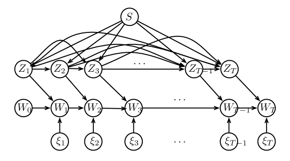
Figure 1: Directed graphical model illustrating dependencies between data set $S$, samples $\{Z_{t}\}$, parameter iterates $\{W_{t}\}$, and noise vectors $\{\xi_{t}\}$.

where $T$ denotes the final iterate. We may represent the dependence structure defined by our class of algorithms in the form of a graphical model (see Figure 1 in the Appendix).

Remark 2.

Importantly, we do not impose any further restrictions on the form of the updates or the sampling strategy; in particular, $Z_{t}$ need not be drawn uniformly from the data set $S$, and may even depend on past iterates $\{Z_{s}\}_{s<t}$, as in the case of sampling without replacement. Some examples of iterative algorithms where the probability of sampling a data point $z_{i}$ depends on the value of $z_{i}$ may be found in Zhao and Zhang [21] or Needell et al. [11]—such sampling strategies are also covered by our theory. However, note that $Z_{t}$ must be independent of the parameter iterates $\{W_{s}\}_{s<t}$, since if edges exist between $W_{t}$ and any $Z_{s}$ such that $s>t$, equation (5) will not hold. Intuitively, if the sampled data point adapts to current iterates of the parameter vector $W_{t}$, the algorithm may be prone to over-fitting and may not generalize.

Finally, note that our assumptions do not require the loss function $\ell$ to satisfy conditions such as convexity. In fact, the way we have defined the updates (3) does not require $F$ to be related to $\ell$ in any way. On the other hand, if $F$ is essentially a gradient of $\ell$, as is often the case, Assumption 2 will be satisfied as long as $\ell$ is Lipschitz in its first argument.

The output of our estimation algorithm is defined to be an arbitrary function of the $T$ iterates: $W=f(W^{(T)})$. Some common examples appearing in the ERM literature include (i) the mean: $f(W^{(T)})=\frac{1}{T}\sum_{t=1}^{T}{W_{t}}$; (ii) the last iterate: $f(W^{(T)})=W_{T}$; or (iii) suffix averaging, and variants thereof [13, 17].

3 Main results

We now derive an upper bound on $I(S;W)$ for the class of iterative algorithms described in Section 2, from which we obtain bounds on the generalization error.

3.1 Bound on mutual information

Theorem 1.

The mutual information satisfies the bound

$$I(S;W) \leq\sum_{t=1}^{T}\frac{d}{2}\log\left(1+\frac{\eta_{t}^{2}L^{2}}{d\sigma_{t}^{2}}\right).$$

Proof.

$$I(S;W) =I(S;f(W^{(T)}))\leq I(S;W^{(T)})$$

$$\leq I(Z^{(T)};W^{(T)})$$

$$=I(Z^{(T)};W_{1})+I(Z^{(T)};W_{2}|W_{1})$$

$$\quad+I(Z^{(T)};W_{3}|W_{1},W_{2})+\cdots+I(Z^{(T)};W_{T}|W^{(T-1)})$$

where the inequality follows from Lemma 2 and the last equality comes from the chain rule of mutual information.

For all $t$,

$$I(Z^{(T)};W_{t}|W^{(t-1)})$$

$$\quad=h(W_{t}|W^{(t-1)})-h(W_{t}|W^{(t-1)},Z^{(T)})$$

$$\quad\stackrel{{\scriptstyle(a)}}{{=}}h(W_{t}|W_{t-1})-h(W_{t}|W_{t-1},Z_{t})$$

$$\quad=I(W_{t};Z_{t}|W_{t-1})$$

$$\quad\stackrel{{\scriptstyle(b)}}{{\leq}}\frac{d}{2}\log\left(1+\frac{\eta_{t}^{2}L^{2}}{d\sigma_{t}^{2}}\right),$$ (6)

where equality $(a)$ follows from Lemma 3 and Lemma 4 in the Appendix, whereas inequality $(b)$ follows from Lemma 5.

Therefore, Eq. (3.1) gives

$$I(S;W^{(T)}) \leq\sum_{t=1}^{T}\frac{d}{2}\log\left(1+\frac{\eta_{t}^{2}L^{2}}{d\sigma_{t}^{2}}\right).$$ (7)

We may obtain bounds without a log term by using the fact that $\log(1+x)\leq\frac{x}{\sqrt{1+x}}<x$, $\forall x>0$. ∎

3.2 Consequences

We now use this bound on mutual information from Theorem 1 to derive bounds on the generalization error, first in expectation and then with high probability. The first bound follows directly from Theorem 1 and Lemma 1:

Corollary 1 (Bound in expectation).

The generalization error of our class of iterative algorithms is bounded by

$$|\text{gen}(\mu,P_{W|S})|\leq\sqrt{\frac{R^{2}}{n}\sum_{t=1}^{T}\frac{\eta_{t}^{2}L^{2}}{\sigma_{t}^{2}}}.$$ (8)

Similarly, Theorem 3 in Xu and Raginsky [20] implies a generalization error bound that holds with high probability:

Corollary 2.

[High-probability bound] Let $I(S;W)\leq\epsilon$. Then by Theorem 1, $\epsilon$ can be equal to $\sum_{t=1}^{T}\frac{d}{2}\log\left(1+\frac{\eta_{t}^{2}L^{2}}{d\sigma_{t}^{2}}\right)$. For any $\alpha>0$ and $0<\beta\leq 1$, if $n>\frac{8R^{2}}{\alpha^{2}}\left(\frac{\epsilon}{\beta}+\log(\frac{2}{\beta})\right)$, we have

$$\mathbb{P}_{S,W}\left(|L_{\mu}(W)-L_{S}(W)|>\alpha\right)\leq\beta,$$ (9)

where the probability is with respect to $S\sim\mu^{\otimes n}$ and $W$.

4 Examples

We now apply the corollaries in Section 3.2 to obtain generalization error bounds for various algorithms.

4.1 SGLD

As mentioned earlier, sampling the data points uniformly and setting $g(w)=w$ and $F(w,z)=\nabla_{w}\ell(w,z)$ corresponds to the SGLD algorithm. Common experimental practices for SGLD are as follows [19]:

1. the noise variance is set to be $\sigma_{t}=\sqrt{\eta_{t}}$,

2. the algorithm is run for $K$ epochs; i.e., $T=nK$,

3. for a constant $c>0$, the stepsizes are $\eta_{t}=\frac{c}{t}$.

High-probability bounds

For a given choice of $\{\beta,\alpha\}$, taking $n\geq\frac{64R^{4}}{\alpha^{4}}\left(\log(\frac{2}{\beta})\right)^{2}$ ensures inequality (9), provided that we run $K\leq\frac{1}{ne}\left(\frac{2}{\beta}^{\frac{2(\sqrt{n}-1)\beta}{cL^{2}}}\right)$ epochs. For more details, see Lemma 6 in Appendix B.

Bounds in expectation

Using the identity $\sum_{t=1}^{T}\frac{1}{t}\leq\log(T)+1$, we obtain the following bound:

$$|\text{gen}(\mu,\mathbb{P}_{W|S})| \leq\frac{RL}{\sqrt{n}}\sqrt{\sum_{t=1}^{T}\eta_{t}}\leq\frac{RL}{\sqrt{n}}\sqrt{c\log T+c}.$$

Note that Mou et al. [9] achieve a tighter bound on generalization error of the order $\mathcal{O}\left(\frac{1}{n}\right)$, but their bound is only applicable to the last iterate $W_{T}$ of SGLD and a uniform sampling strategy.

Convex risk minimization

If the loss function $\ell(w,z)$ is convex in its first argument for every $w$, we may also bound the excess risk of the learning algorithm. Recall the bound (1) and the definition of the optimization error. It may be shown (cf. Lemma 7 in Appendix B) that when $(\eta_{t},\sigma_{t})=(\eta,\sigma)$ and $W=\frac{1}{T}\sum_{t=1}^{T}W_{t}$, the optimization error of SGLD satisfies

$$\epsilon_{\text{opt}}^{W}\leq\frac{G^{2}}{2\eta T}+\frac{\eta}{2}L^{2}+\frac{d\sigma^{2}}{2\eta},$$ (10)

where $G=\sup_{w,S}\|w_{0}-w^{*}_{S}\|_{2}$. By inequalities (1), (4.3), and (10), we then have

$$\mathop{{}\mathbb{E}}[L_{S}[W]] \leq L(w^{*})+\frac{G^{2}}{2\eta T}+\frac{\eta}{2}L^{2}+\frac{d\sigma^{2}}{2\eta}+\frac{R\sqrt{T}}{\sqrt{n}}\frac{\eta L}{\sigma}.$$

Setting $\sigma=\frac{G}{\sqrt{dT}}$ and $\eta=\sqrt{\frac{G^{2}}{TL(\frac{L}{2}+\frac{R\sqrt{d}T}{\sqrt{n}G})}}$, we obtain

$$\mathop{{}\mathbb{E}}[L_{S}[W]]-L(w^{*}) \leq 2GL\sqrt{\frac{1}{2T}+\frac{\sqrt{d}}{\sqrt{n}}\frac{R}{GL}}.$$

4.2 Perturbed SGD

Due to the requirement that an independent noise term $\xi_{t}$ is present in each update, our results on generalization error may not be applied to SGD. On the other hand, our framework does apply to noisy versions of SGD, which have recently drawn interest in the optimization literature due to their ability to escape saddle points efficiently [5, 7]. For a stepsize parameter $\eta>0$, updates of the perturbed SGD algorithm take the following form [5]:

$$W_{t}=W_{t-1}-\eta\left(\nabla_{w}\ell(W_{t-1},Z_{t})+\xi_{t}\right),$$ (11)

where $\xi_{t}$ are i.i.d. noise terms sampled uniformly from the unit sphere. Hence, noise is added to each gradient. Unfortunately, our techniques cannot be applied to this exact setting because $\xi_{t}$ has a degenerate distribution concentrated on the sphere. For large enough $d$, choosing $\xi_{t}$ on the unit sphere is almost equivalent to choosing it inside the unit ball. If $\xi_{t}$ is chosen uniformly in the unit ball (cf. the perturbed SGD formulation in Jin et al. [7]), our methods yield the following bound:

$$I(S;W)\leq Td\log(1+L).$$ (12)

This is because $\|W_{t}-W_{t-1}\|_{2}\leq\eta(L+1)$, so we may bound $h(W_{t}|W_{t-1})$ by the entropy of the uniform distribution on the $d$-dimensional ball of radius $\eta(L+1)$. Also, $h(W_{t}|W_{t-1},Z_{t})$ is simply the entropy of the uniform distribution on the $d$-dimensional ball of radius $\eta$. This shows that $I(W_{t};Z_{t}|W_{t-1})\leq d\log(1+L)$, so

$$I(W;S)\leq I(W^{(T)};S)\leq I(W^{(T)};Z^{(T)})\leq Td\log(1+L).$$

4.3 Noisy momentum

In this section, we show how we can develop bounds for momentum-like algorithms in addition to SGLD. We consider an algorithm similar to the SGHMC algorithm [3]. Every iteration $t$ involves an extra parameter vector $V_{t}$, which represents the “velocity” of $W_{t}$. We analyze a modified SGHMC algorithm, where we add the (independent and Gaussian) noise $\xi^{\prime}_{t}$ to the velocity, as well. This leads to the update equations

$$\begin{aligned} V_{t}&=\gamma_{t}V_{t-1}+\eta_{t}\nabla_{w}\ell(W_{t-1},Z_{t})+\xi^{\prime}_{t},\\ W_{t}&=W_{t-1}-\gamma_{t}V_{t-1}-\eta_{t}\nabla_{w}\ell(W_{t-1},Z_{t})+\xi^{\prime\prime}_{t},\end{aligned}$$ (13)

or in matrix form,

$$\begin{bmatrix}V_{t}\\ W_{t}\end{bmatrix} =\begin{bmatrix}\gamma_{t}&0\\ -\gamma_{t}&1\end{bmatrix}\begin{bmatrix}V_{t-1}\\ W_{t-1}\end{bmatrix}+\eta_{t}\begin{bmatrix}\nabla_{w}\ell(W_{t-1},Z_{t})\\ -\nabla_{w}\ell(W_{t-1},Z_{t})\end{bmatrix}+\begin{bmatrix}\xi^{\prime}_{t}\\ \xi^{\prime\prime}_{t}\end{bmatrix}.$$

Thus, we may recast the updates in the framework of our paper by treating $(V_{t},W_{t})$ as a single parameter vector in $\mathbb{R}^{2d}$, with

$$g(V_{t-1},W_{t-1}) =\begin{bmatrix}\gamma_{t}&0\\ -\gamma_{t}&1\end{bmatrix}\begin{bmatrix}V_{t-1}\\ W_{t-1}\end{bmatrix},\quad\text{and}$$

$$F\big{(}(V_{t-1},W_{t-1}),Z_{t}\big{)} =\begin{bmatrix}\nabla_{w}\ell(W_{t-1},Z_{t})\\ -\nabla_{w}\ell(W_{t-1},Z_{t})\end{bmatrix}.$$

Note that if the gradients are upper-bounded by $L$, we have $\sup_{v,w\in\mathcal{W},z\in\mathcal{Z}}\|F((v,w),z)\|_{2}\leq\sqrt{2}L$. Using Theorem 1, we then arrive at the following bound:

$$I(S;W) \leq\sum_{t=1}^{T}\frac{2d}{2}\log\left(1+\frac{\eta_{t}^{2}2L^{2}}{2d\sigma_{t}^{2}}\right).$$

Note that it is twice the bound on the mutual information appearing in Theorem 1. We may then apply the results in Section 3.2 to obtain bounds on the generalization error:

$$|\text{gen}(\mu,P_{W|S})|\leq\sqrt{\frac{2R^{2}}{n}\sum_{t=1}^{T}\frac{\eta_{t}^{2}L^{2}}{\sigma_{t}^{2}}}.$$

4.4 Accelerated gradient descent

Finally, we consider a noisy version of the accelerated gradient descent method of Nesterov [12], where we again add independent noise to both the velocity and parameter vectors at each iteration. This leads to the update equations

$$\begin{aligned} V_{t+1}&=\gamma V_{t}+\eta_{t}\nabla_{w}\ell(W_{t}-\gamma_{t}V_{t},Z_{t})+\xi^{\prime}_{t+1},\\ W_{t+1}&=W_{t}-V_{t+1}+\xi^{\prime\prime}_{t+1}+\xi^{\prime}_{t+1}.\end{aligned}$$

We again consider $(V_{t},W_{t})$ as a single parameter vector in $\mathbb{R}^{2d}$. Compared with the updates (13), we see that the only difference is that the point where we take the gradient has changed. Therefore, we obtain the same bound on the $F\big{(}(V_{t-1},W_{t-1}),Z_{t}\big{)}$ as in the case of noisy momentum: $\sup_{v,w\in\mathcal{W},z\in\mathcal{Z}}\|F((v,w),z)\|_{2}\leq\sqrt{2}L$. This leads to the same upper bound on the mutual information (and generalization error) as in the previous subsection.

5 Conclusion

In this paper, we have demonstrated that mutual information is a very effective tool for bounding the generalization error of a large class of iterative ERM algorithms. The simplicity of our analysis is due to properties such as the data processing inequality and the chain rule of mutual information. However, entropy and mutual information also have certain shortcomings that limit the scope of our analysis, particularly concerning the sensitivity of entropy with respect to degenerate random variables. In some instances, mutual information-based bounds become very weak or even inapplicable. For example, if we were to analyze the SGD algorithm rather than SGLD, or add noise that is degenerate, such as the uniform distribution on a sphere [5], the mutual information $I(W;S)$ would be $+\infty$, leading to meaningless generalization error bounds. It would be interesting to develop information-theoretic strategies that could bound the generalization error for such algorithms, as well. Finally, note that we have only provided upper bounds for the generalization error—having a large $I(W;S)$ does not necessarily mean that an algorithm is overfitting, since our upper bound might be loose. Deriving lower bounds on the generalization error appears to be a challenging problem that could benefit from an information-theoretic approach, as well.

Appendix A Proofs of supporting lemmas to Theorem 1

We now prove the lemmas employed in the proof of Theorem 1.

Lemma 2.

$I(S;W)\leq I(Z^{(T)};W^{(T)})$.

Proof.

This follows from the Markov chain

$$S\rightarrow Z^{(T)}\rightarrow W^{(T)}.$$

See equality (5). ∎

Lemma 3.

For all $t$, we have

$$h(W_{t}|W^{(t-1)},Z^{(T)})=h(W_{t}|W_{t-1},Z_{t}).$$

Proof.

This follows from the Markov chain

$$(W^{(t-2)},Z^{(T)\backslash\{t\}})\rightarrow(W_{t-1},Z_{t})\rightarrow W_{t},$$

where $Z^{(T)\backslash\{t\}}:=(Z_{1},\ldots,Z_{t-1},Z_{t+1},\ldots,Z_{T})$. See equality (5). ∎

Lemma 4.

For all $t$, we have

$$h(W_{t}|W^{(t-1)})=h(W_{t}|W_{t-1}).$$

Proof.

This follows from the Markov chain

$$W^{(t-2)}\rightarrow W_{t-1}\rightarrow W_{t}.$$

See equality (5). ∎

Lemma 5.

For all $t$, we have

$$I(W_{t};Z_{t}|W_{t-1})\leq\frac{d}{2}\log\left(1+\frac{\eta_{t}^{2}L^{2}}{d\sigma_{t}^{2}}\right).$$

Proof.

Note that

$$I(W_{t};Z_{t}|W_{t-1})=h(W_{t}|W_{t-1})-h(W_{t}|W_{t-1},Z_{t}).$$

We now bound each of the terms in the final expression. First, note that conditioned on $W_{t-1}=w_{t-1}$, we have

$$W_{t}-g(w_{t-1})=\eta_{t}F(w_{t-1},Z_{t})+\xi_{t}.$$

Note that

$$h(W_{t}-g(w_{t-1})\mid W_{t-1})=h(W_{t}\mid W_{t-1}=w_{t-1}),$$

since translation does not affect the entropy of a random variable. Also note that the random variables $\xi_{t}$ and $\eta_{t}F(w_{t-1},Z_{t})$ are independent, so we can upper-bound the expected squared-norm of $W_{t}-w_{t-1}$, as follows:

$$\mathop{{}\mathbb{E}}\left(\|W_{t}-w_{t-1}\|_{2}^{2}\right) =\mathop{{}\mathbb{E}}\left(\|\eta_{t}F(w_{t-1},Z_{t})\|_{2}^{2}+\|\xi_{t}\|_{2}^{2}\right)$$

$$\leq\eta_{t}^{2}L^{2}+d\sigma_{t}^{2},$$

where in the last inequality, we have used Assumption 2 and the fact that $\xi_{t}\sim{\cal N}(0,\sigma_{t}^{2}I_{d})$. Among all random variables $X$ with a fixed $\mathbb{E}\|X\|_{2}^{2}<C$, the Gaussian distribution $Y\sim{\cal N}\left(0,\sqrt{\frac{C}{d}}I_{d}\right)$ has the largest entropy, given by

$$h(Y)=\frac{d}{2}\log\left(\frac{2\pi eC}{d}\right).$$

This implies that

$$h(W_{t}\mid W_{t-1}=w_{t-1}) \leq\frac{d}{2}\log\left(2\pi e\frac{\eta_{t}^{2}L^{2}+d\sigma_{t}^{2}}{d}\right).$$

Since the above bound holds for all values $w_{t-1}$, we may integrate the bound to conclude that

$$h(W_{t}|W_{t-1})\leq\frac{d}{2}\log\left(2\pi e\frac{\eta_{t}^{2}L^{2}+d\sigma_{t}^{2}}{d}\right).$$

We also have

$$h(W_{t}|W_{t-1},Z_{t}) =h(W_{t-1}+\eta_{t}\nabla_{w}\ell(W_{t-1},Z_{t})$$

$$\quad+\xi_{t}|W_{t-1},Z_{t})$$

$$=h(\xi_{t}|W_{t-1},Z_{t})$$

$$=h(\xi_{t}).$$

This leads to the following desired bound:

$$h(W_{t}|W_{t-1}) -h(W_{t}|Z_{t},W_{t-1})$$

$$\leq\frac{d}{2}\log\left(2\pi e\frac{\eta_{t}^{2}L^{2}+d\sigma_{t}^{2}}{d}\right)-\frac{d}{2}\log 2\pi e\sigma_{t}^{2}$$

$$=\frac{d}{2}\log\frac{\eta_{t}^{2}L^{2}+d\sigma_{t}^{2}}{d\sigma_{t}^{2}}$$

$$=\frac{d}{2}\log\left(1+\frac{\eta_{t}^{2}L^{2}}{d\sigma_{t}^{2}}\right).$$

Note that if the noise were non-Gaussian, we would have to replace $\frac{d}{2}\log(2\pi e\sigma_{t}^{2})$ by the entropy of the noise. ∎

Appendix B Details for the SGLD algorithm

In this Appendix, we include more details for the derivations concerning SGLD in Section 4.

B.1 Generalization error bounds

Lemma 6.

For a given choice of $\{\beta,\alpha\}$, taking $n\geq\frac{64R^{4}}{\alpha^{4}}(\log(\frac{2}{\beta}))^{2}$ ensures inequality (9), provided that we run $K\leq\frac{1}{ne}\left(\frac{2}{\beta}^{\frac{2(\sqrt{n}-1)\beta}{cL^{2}}}\right)$ epochs.

Proof.

If we show that for $K\leq\frac{1}{ne}\left(\frac{2}{\beta}^{\frac{2(\sqrt{n}-1)\beta}{cL^{2}}}\right)$, we have $I(S;W)\leq(\sqrt{n}-1)\beta\log\left(\frac{2}{\beta}\right)$, the proof will follow from Corollary 2. We have

$$I(S;W) \leq\sum_{t=1}^{T}\frac{\eta L^{2}}{2}=\sum_{t=1}^{T}\frac{cL^{2}}{2t}\leq\frac{cL^{2}}{2}\log(eT)$$

$$=\frac{cL^{2}}{2}\log(enK)$$

$$\leq\frac{cL^{2}}{2}\log\left(\frac{2}{\beta}^{\frac{2(\sqrt{n}-1)\beta}{cL^{2}})}\right)$$

$$=(\sqrt{n}-1)\beta\log\left(\frac{2}{\beta}\right),$$

implying the desired result. ∎

B.2 Optimization error bounds

We now derive the bound on the optimization error $\epsilon_{\text{opt}}^{W}$ of SGLD.

Lemma 7.

If we run the SGLD algorithm on an $L$-Lipschitz convex loss function for $T$ time steps with parameters $\{\eta,\sigma\}$, we have the following bound on the empirical risk for the average of the iterates:

$$\mathop{{}\mathbb{E}}\left[L_{S}\left(\frac{1}{T}\sum_{t=1}^{T}W_{t}\right)\right]-L_{S}(w_{S}^{*})\leq\mathop{{}\mathbb{E}}\left[\frac{1}{T}\sum_{t=1}^{T}L_{S}(W_{t})\right]-L_{S}(w_{S}^{*})\leq\frac{G^{2}}{2\eta T}+\frac{\eta}{2}L^{2}+\frac{d\sigma^{2}}{2\eta}.$$

We follow the same notation as in the rest of the paper.

Proof.

The first inequality follows from the convexity of the the loss fuction.

We can write the update equation as

$$W_{t} =W_{t-1}-\eta\left(\nabla_{w}\ell(W_{t-1},Z_{t})+\frac{\xi}{\eta}\right)$$

$$=W_{t-1}-\eta V_{t-1},$$

where $V_{t}=\nabla_{w}\ell(W_{t-1},Z_{t})+\frac{\xi}{\eta}$.

It is easy to see that $V_{t}$ is an unbiased estimator of the gradient of the empirical risk; i.e., $\mathop{{}\mathbb{E}}[V_{t}|W_{t}]=\nabla L_{S}(W_{t})$. Therefore, SGLD may be seen as a variant of SGD, and we obtain the following bounds on the optimization error for the average of iterates, $W=\frac{1}{T}\sum_{t=1}^{T}W_{t}$ (cf. Lemma 14.1 and Theorem 14.8 of Shalev-Shwartz and Ben-David [15]):

$$\epsilon_{\text{opt}}^{W}\leq\frac{G^{2}}{2\eta T}+\frac{\eta}{2}(\mathop{{}\mathbb{E}}[\|V_{t}\|_{2}^{2}]).$$ (14)

Moreover, since the noise is independent and the loss function is convex and $L$-Lipschitz, we have

$$\mathop{{}\mathbb{E}}[\|V_{t}\|_{2}^{2}]\leq L^{2}+d\frac{\sigma^{2}}{\eta^{2}}.$$

Combining this bound with inequality (14) yields the desired result. ∎

References

- [1] S. Boucheron, G. Lugosi, and P. Massart. Concentration Inequalities: A Nonasymptotic Theory of Independence. Oxford University Press, 2013.
- [2] O. Bousquet and A. Elisseeff. Stability and generalization. Journal of Machine Learning Research, 2:499–526, March 2002.
- [3] T. Chen, E. Fox, and C. Guestrin. Stochastic gradient Hamiltonian Monte Carlo. In E. P. Xing and T. Jebara, editors, Proceedings of the 31st International Conference on Machine Learning, volume 32 of Proceedings of Machine Learning Research, pages 1683–1691. PMLR, 2014.
- [4] A. Elisseeff, T. Evgeniou, and M. Pontil. Stability of randomized learning algorithms. Journal of Machine Learning Research, 6:55–79, December 2005.
- [5] R. Ge, F. Huang, C. Jin, and Y. Yuan. Escaping from saddle points—Online stochastic gradient for tensor decomposition. In Conference on Learning Theory, pages 797–842, 2015.
- [6] M. Hardt, B. Recht, and Y. Singer. Train faster, generalize better: Stability of stochastic gradient descent. In M. F. Balcan and K. Q. Weinberger, editors, Proceedings of The 33rd International Conference on Machine Learning, volume 48, pages 1225–1234, New York, New York, USA, 20–22 Jun 2016. PMLR.
- [7] C. Jin, R. Ge, P. Netrapalli, S. M. Kakade, and M. I. Jordan. How to escape saddle points efficiently. arXiv preprint:1703.00887, 2017.
- [8] B. London. Generalization bounds for randomized learning with application to stochastic gradient descent. In NIPS Workshop on Optimizing the Optimizers, 2016.
- [9] W. Mou, L. Wang, X. Zhai, and K. Zheng. Generalization bounds of SGLD for non-convex learning: Two theoretical viewpoints. CoRR, 2017.
- [10] S. Mukherjee, P. Niyogi, T. Poggio, and R. Rifkin. Learning theory: Stability is sufficient for generalization and necessary and sufficient for consistency of empirical risk minimization. Advances in Computational Mathematics, 25(1):161–193, Jul 2006.
- [11] D. Needell, N. Srebro, and R. Ward. Stochastic gradient descent, weighted sampling, and the randomized Kaczmarz algorithm. Mathematical Programming, 155(1–2):549–573, January 2016.
- [12] Yurii Nesterov. A method of solving a convex programming problem with convergence rate . Soviet Mathematics Doklady, 27:372–376, 1983.
- [13] A. Rakhlin, O. Shamir, and K. Sridharan. Making gradient descent optimal for strongly convex stochastic optimization. In ICML, 2012.
- [14] D. Russo and J. Zou. Controlling bias in adaptive data analysis using information theory. In A. Gretton and C. C. Robert, editors, Proceedings of the 19th International Conference on Artificial Intelligence and Statistics, volume 51 of Proceedings of Machine Learning Research, pages 1232–1240. PMLR, 09–11 May 2016.
- [15] S. Shalev-Shwartz and S. Ben-David. Understanding Machine Learning: From Theory to Algorithms. Cambridge University Press, New York, NY, USA, 2014.
- [16] S. Shalev-Shwartz, O. Shamir, N. Srebro, and K. Sridharan. Learnability, stability and uniform convergence. Journal of Machine Learning Research, 11:2635–2670, December 2010.
- [17] O. Shamir and T. Zhang. Stochastic gradient descent for non-smooth optimization: Convergence results and optimal averaging schemes. In International Conference on Machine Learning, pages 71–79, 2013.
- [18] V. N. Vapnik. Statistical Learning Theory. Wiley-Interscience, 1998.
- [19] M. Welling and Y. W. Teh. Bayesian learning via stochastic gradient Langevin dynamics. In Proceedings of the 28th International Conference on Machine Learning (ICML-11), pages 681–688, 2011.
- [20] A. Xu and M. Raginsky. Information-theoretic analysis of generalization capability of learning algorithms. In I. Guyon, U. V. Luxburg, S. Bengio, H. Wallach, R. Fergus, S. Vishwanathan, and R. Garnett, editors, Advances in Neural Information Processing Systems, pages 2521–2530. Curran Associates, Inc., 2017.
- [21] P. Zhao and T. Zhang. Stochastic optimization with importance sampling for regularized loss minimization. In Proceedings of the 32Nd International Conference on International Conference on Machine Learning - Volume 37, ICML’15, pages 1–9, 2015.