Computing the density of states for optical spectra by low-rank and QTT tensor approximation

Abstract

In this paper, we introduce a new interpolation scheme to approximate the density of states (DOS) for a class of rank-structured matrices with application to the Tamm-Dancoff approximation (TDA) of the Bethe-Salpeter equation (BSE). The presented approach for approximating the DOS is based on two main techniques. First, we propose an economical method for calculating the traces of parametric matrix resolvents at interpolation points by taking advantage of the block-diagonal plus low-rank matrix structure described in [6, 3] for the BSE/TDA problem. Second, we show that a regularized or smoothed DOS discretized on a fine grid of size $N$ can be accurately represented by a low rank quantized tensor train (QTT) tensor that can be determined through a least squares fitting procedure. The latter provides good approximation properties for strictly oscillating DOS functions with multiple gaps, and requires asymptotically much fewer ($O(\log N)$) functional calls compared with the full grid size $N$. This approach allows us to overcome the computational difficulties of the traditional schemes by avoiding both the need of stochastic sampling and interpolation by problem independent functions like polynomials etc. Numerical tests indicate that the QTT approach yields accurate recovery of DOS associated with problems that contain relatively large spectral gaps. The QTT tensor rank only weakly depends on the size of a molecular system which paves the way for treating large-scale spectral problems.

Key words: Bethe-Salpeter equation, density of states, absorption spectrum, tensor decompositions, model reduction, low-rank matrix, QTT tensor approximation.

AMS Subject Classification: 65F30, 65F50, 65N35, 65F10

1 Introduction

Numerical approximation of the density of states (DOS) or spectral density (see §2.2) of large matrices is one of the challenging problems arising in the prediction of electronic, vibrational and thermal properties of molecules and crystals and many other applications. This topic, first developed in condensed matter physics [14, 44, 41, 13, 43], has long since attracted interest in the community of numerical linear algebra [42, 16, 40], see also a survey on commonly used methodology for approximation of DOS for large matrices of general structure [25]. Most traditional methods are based on a polynomial or fractional-polynomial interpolation of the DOS regularized by Gaussians or Lorentzians, and computing traces of certain matrix valued functions, say matrix resolvents or polynomials, defined at a large set of interpolation points within the spectral interval of interest. Furthermore, the trace calculations are typically accomplished with stochastic sampling over a large number of random vectors [25].

Since the size of matrices resulting from real life applications is usually large (in quantum mechanics it scales as a polynomial of the molecular size), and the DOS of these matrices often exhibits very complicated shape, the above mentioned methods become prohibitively expensive. Moreover, the algorithms based on polynomial interpolants have poor approximating properties when the spectrum of a matrix exhibits gaps or highly oscillating non-regular shapes, as is the case in electronic structure calculations. Furthermore, stochastic sampling leads to poor Monte Carlo estimates with slow convergence rates and low accuracy.

In this paper we present a new method to efficiently and accurately approximate the DOS for large rank-structured symmetric matrices. The approach amounts to estimating the DOS by evaluating matrix functions of structured matrices, in particular traces of the matrix resolvent. Our main contribution is to perform each function evaluation at low cost and to reduce the total number of function evaluations in the case of fine representation grid.

We apply this approximation to the Bethe-Salpeter equation (BSE), which is a widely used model for ab initio estimation of the absorption spectra for molecules or surfaces of solids [35, 18, 39, 32, 27, 31]. In particular, we use the recently developed low-rank structured representation of the BSE Hamiltonian, which was introduced and analyzed in [6]. An efficient and structured eigenvalue solver for this block-diagonal plus low-rank representation of the BSE Hamiltonian as well as to its symmetric positive definite surrogate obtained by the Tamm-Dancoff approximation (TDA) is described in [3].

The approach we take here to approximate the DOS of the BSE Hamiltonian relies on the Lorentzian blurring [17]. The most computationally expensive part of the calculation is reduced to the evaluation of traces of shifted matrix inverses. Our method is based on two main ingredients. First, we propose an economical method for calculating traces of parametric matrix resolvents at interpolation points by taking advantage of the block-diagonal plus low-rank BSE/TDA matrix structure described in [6, 3], which enables the direct inversion of the shifted Hamiltonian within the same matrix structure. This allows us to overcome the computational difficulties of the traditional schemes and avoid the need of stochastic sampling. Second, we show that a regularized or smoothed DOS can be accurately approximated by a low rank QTT tensor [23] that can be determined through a least squares procedure. The accuracy of approximation and interpolation is controlled by $\epsilon$-truncation of the corresponding matrix/tensor ranks.

Our fast method for calculating traces of matrix resolvents for the family of rank-structured matrices exhibits almost linear asymptotic complexity scaling with respect to the matrix size. We introduce an explicit rank-structured representation of the matrix inverse which can be evaluated efficiently by using the Sherman-Morrison-Woodbury formula. Note that the diagonal plus low-rank approximation to the BSE Hamiltonian introduced in [6] employs the low-rank approximation to the two-electron integrals tensor in the form of a Cholesky factorization [21]. An efficient structured solver designed to calculate a number of minimal eigenvalues of the block-diagonal plus low-rank representation of the BSE/TDA matrices is described in [3].

Another novelty of this paper is the application of the QTT tensor approximation to the DOS sampled on a fine grid, which results in a long vector. The QTT approximation method was introduced and analyzed for function related vectors in [23]. It was proven that for a length-$N$ vector obtained from the discretization of a classical function (complex exponentials, polynomials, Gaussians etc.), its QTT image constructed in the $L$-dimensional tensor space with $L=\log_{2}N$ exhibits an amazingly low separation rank $r_{qtt}$. This rank parameter $r_{qtt}$ appears to be independent of the size of the original vector. Thus the use of QTT tensor compression reduces the number of representation parameters from $N$ to $2r_{qtt}^{2}\log_{2}N$, which allows asymptotically a much smaller number of functional calls, $O(\log N)$, to reconstruct the DOS function in the QTT parametrization. This might be beneficial in the limit of a large number of representation points $N$ since each functional evaluation of the DOS is highly expensive requiring computation of some matrix valued functions.

For example, for a vector of size $N=2^{L}$ representing the exponential function, its reshape (folding) into an $L$-dimensional tensor of size ${\underbrace{2\times\cdots\times 2}}_{L-fold}$ with modes equal to $2$, yields a QTT tensor of rank $r_{qtt}=1$, which means the reduction of storage from $2^{L}$ to $2\log_{2}N=2L$. For a complex exponential vector there holds $r_{qtt}=2$, then storage reduces from $N$ to $8\log_{2}N$. Similar low rank QTT representations were proven for a wide class of functions [24], including strongly oscillating functions of nontrivial shape, see for example [19, 22] and the new results in §4.4 below. For a general class of functional vectors, one computes an $\varepsilon$-rank QTT approximation which leads to a storage size with logarithmic scaling in $N$.

Numerical tests for moderate size molecules confirm the closeness of DOS for the TDA model to those computed on the exact BSE spectrum. We also justify that the simplified block-diagonal plus low-rank approximation recovers well the main landscape and shape details of the DOS curve on the whole energy interval and check the precision of the low-rank QTT approximation to the length-$N$ vector representing the DOS. We demonstrate the almost linear complexity scaling of the trace calculation algorithm applied to TDA matrices of different size. We then show by numerical tests that the low-rank QTT tensor interpolation scheme requires only a small number of adaptively chosen samples in the $N$-vector discretizing the DOS. For instance, a polynomial interpolant of degree $p$ needs $p+1$ interpolation points (functional calls) for the representation of a function on a large $N$-grid. However, in the case of highly oscillating DOS functions of interest one should impose $p=O(N)$. On the contrary, the QTT interpolant over $O(\log N)$ interpolation points provides a rather accurate representation of the functional $N$-vector of the DOS.

We also discuss the opportunity to reduce the cost of multiple trace calculations for the parametric matrix resolvent and, finally, describe modifications necessary to calculate the optical absorption spectrum via a rank-structured BSE model.

The rest of the paper is structured as follows. In Section 2, we recall the main prerequisites for the description of our method including the rank-structured approximation to the BSE/TDA matrix, basic notions of the regularization of DOS by Lorentzians and a short summary on the existing methods for matrices of general structure. Section 3 discusses the main techniques of the presented method and the corresponding analysis in Theorems 3.1 and 3.2. The numerical tests confirm the linear scaling of our algorithm in the size of the grid on which the DOS is evaluated. Section 4 presents a summary of the QTT tensor approximation of function related vectors and the analysis of the QTT tensor ranks of the DOS, see Theorem 4.1. In Section 4.3 the ACA based QTT interpolation is applied to the discretized DOS, where the quality of the interpolation is illustrated numerically. The beneficial features of the new computational schemes are verified by extensive numerical experiments on the examples of various molecular systems. Section 5 outlines the extension of the approach to the case of full BSE system. Conclusions summarize the main results and address the application perspectives.

2 Main prerequisites and outline of initial applications

2.1 Rank-structured approximation to BSE matrix

In this paper we describe a method for efficient and accurate approximation of the DOS for large rank-structured symmetric matrices. Our basic application is concerned with estimating the DOS and the absorption spectrum for the Bethe-Salpeter problem describing the excitation energies of molecules.

The $2\times 2$-block matrix representation of the Bethe-Salpeter Hamiltonian (BSH) leads to the following eigenvalue problem.

$$H\begin{pmatrix}{\bf x}_{k}\\ {\bf y}_{k}\\ \end{pmatrix}\equiv\begin{pmatrix}{A}&{B}\\ {-B}^{\ast}&{-A}^{\ast}\\ \end{pmatrix}\begin{pmatrix}{\bf x}_{k}\\ {\bf y}_{k}\\ \end{pmatrix}=\omega_{k}\begin{pmatrix}{\bf x}_{k}\\ {\bf y}_{k}\\ \end{pmatrix},$$ (2.1)

where the matrix blocks of size $n\times n$, with $n=N_{ov}=N_{o}(N_{b}-N_{o})$, are defined by

$$A=\boldsymbol{\Delta\varepsilon}+V-\widehat{W},\quad B={V}-\widetilde{W},$$ (2.2)

and eigenvalues $\omega_{k}$ correspond to the excitation energies. Here $\boldsymbol{\Delta\varepsilon}$ is a diagonal matrix and

$${V}=[v_{ia,jb}]\quad a,b\in{\cal I}_{v}:=\{N_{o}+1,\ldots,N_{b}\},\quad i,j\in{\cal I}_{o}:=\{1,\ldots,N_{o}\},$$

is the rank-$R_{B}$ two-electron integrals (TEI) matrix projected onto the Hartree-Fock molecular orbital basis, where $N_{b}$ is the number of Gaussian type orbital (GTO) basis functions and $N_{o}$ denotes the number of occupied orbitals [6].

The method for solving the Bethe-Salpeter equation (BSE) using low-rank factorizations of the generating matrices has been introduced in [6]. It is based on a tensor-structured grid-based Hartree-Fock (HF) solver which provides not only the full set of eigenvalues and HF orbitals, but also the two-electron integrals tensor in the form of a low-rank Cholesky factorization, see [20] and references therein.

The matrix $V$ inherits its low rank from the two-electron integrals tensor, and $\widetilde{W}$ is also proven to have a small $\epsilon$-rank (see [6]). In particular, there holds

$$V\approx L_{V}L_{V}^{T},\quad L_{V}\in\mathbb{R}^{n\times R_{V}},\quad R_{V}\leq R_{B},$$ (2.3)

with the rank estimates $R_{V}=R_{V}(\varepsilon)=\mathcal{O}(N_{b}|\log\varepsilon|)$, and $\mathop{\mathrm{rank}}(\widetilde{W})\leq\mathop{\mathrm{rank}}(V)$.

In [3], it was shown that the matrix $\widehat{W}$, which does not exhibit an accurate low rank representation, can be well approximated by a block diagonal matrix

$$\widehat{W}\approx\mbox{blockdiag}[\widehat{B},D],$$

where $\widehat{B}$ is a $N_{W}\times N_{W}$ dense block with $N_{W}=O(n^{\alpha})$, $\alpha<1$. The size of $N_{W}$ is nearly the same as the rank parameter of $L_{V}$. As a result, the TDA matrix $A$ can be approximated by a sum of a block-diagonal matrix and a low rank matrix shown in Figure 2.1, i.e.,

$$A\approx\widehat{A}=\boldsymbol{\Delta\varepsilon}+QQ^{T}-\mbox{blockdiag}[\widehat{B},D]\equiv\mbox{blockdiag}[{B}_{0},D_{0}]+QQ^{T}.$$

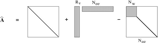
Figure 2.1: Diagonal plus low-rank plus reduced-block structure of the matrix $\widehat{A}$.

An efficient structured solver designed to calculate a number of minimal eigenvalues of the block-diagonal plus low-rank representation of the BSE/TDA matrices is described in [3]. It is based on an efficient subspace iteration of the matrix inverse, which for rank-structured matrix formats can be evaluated efficiently by using the Sherman-Morrison-Woodbury formula, thus reducing the numerical expense of the direct diagonalization down to $\mathcal{O}(N_{b}^{2})$ in the size of the atomic orbitals basis set, $N_{b}$. Furthermore, this solver also includes a QTT-based compression scheme, where both eigenvectors and the rank-structured BSE matrix blocks are represented by block-QTT tensors. The block-QTT representation of the eigenvector is determined by an alternating least squares (ALS) iterative algorithm. The overall asymptotic complexity for computing several smallest in modulo eigenvalues in the BSE spectral problem by using the QTT approximation is estimated to be $\mathcal{O}(\log(N_{o})N_{o}^{2})$, where $N_{o}$ is the number of occupied orbitals.

Matrices in the form (2.1) are called $J$-symmetric or Hamiltonian, see [5] for implications on the algebraic properties of the BSE matrix. In particular, solutions of equation (2.1) come in pairs: excitation energies $\omega_{k}$ with eigenvectors $({\bf x}_{k},{\bf y}_{k})$, and de-excitation energies $-\omega_{k}$ with eigenvectors $({\bf y}_{k}^{\ast},{\bf x}_{k}^{\ast})$.

The simplification in the BSH, $H$, defined by the $n\times n$ symmetric diagonal block $A$ is called the Tamm-Dancoff (TDA) approximation. In what follows, we are interested in the TDA spectral problem,

$$A{\bf u}_{k}=\lambda_{k}{\bf u}_{k},\quad k=1,\ldots,n,$$

providing good approximations to $\omega_{k},{\bf x}_{k}$.

In general, methods for solving partial eigenvalue problems for matrices with a special structure as in the BSE setting are conceptually related to the approaches for Hamiltonian matrices [4, 7, 15, 9], particularly to those based on minimization principles [1, 2]. A structured Lanczos algorithm for estimation of the optical absorption spectrum was described in [37]. Various structured eigensolvers tailored for electronic structure calculations are discussed in [33, 34, 10, 26, 25, 38].

2.2 Density of states for symmetric matrices

To fix the idea, we first consider the case of symmetric matrices. Following [25], we use the simple definition of the DOS for symmetric matrices

$$\phi(t)=\frac{1}{n}\sum\limits_{j=1}^{n}\delta(t-\lambda_{j}),\quad t,\lambda_{j}\in[0,a],$$ (2.4)

where $\delta$ is the Dirac distribution and the $\lambda_{j}$’s are the eigenvalues of $A=A^{T}$ ordered as $\lambda_{1}\leq\lambda_{2}\leq\cdots\leq\lambda_{n}$.

Several classes of blurring approximations to $\phi(t)$ are used in the literature. One can replace each Dirac-$\delta$ by a Gaussian function with width $\eta>0$, i.e.,

$$\delta(t)\rightsquigarrow g_{\eta}(t)=\frac{1}{\sqrt{2\pi}\eta}\exp{\left(-\frac{t^{2}}{2\eta^{2}}\right)},$$

where the choice of the regularization parameter $\eta$ depends on the particular problem setting. As a result, (2.4) can be approximated by

$$\phi(t)\approx\phi_{\eta}(t):=\frac{1}{n}\sum\limits_{j=1}^{n}g_{\eta}(t-\lambda_{j}),$$ (2.5)

on the whole energy interval $[0,a]$.

We may also replace each Dirac-$\delta$ by a Lorentzian, i.e.,

$$\delta(t)\rightsquigarrow L_{\eta}(t):=\frac{1}{\pi}\frac{\eta}{t^{2}+\eta^{2}}=\frac{1}{\pi}\mbox{Im}\left(\frac{1}{t-i\eta}\right),$$ (2.6)

so that an approximate DOS can be written as

$$\phi(t)\approx\phi_{\eta}(t):=\frac{1}{n}\sum\limits_{j=1}^{n}L_{\eta}(t-\lambda_{j}).$$ (2.7)

When $\eta\to 0_{+}$, both Gaussians and Lorentzians converge to the Dirac distribution, i.e.,

$$\lim\limits_{\eta\to 0_{+}}g_{\eta}(t)=\lim\limits_{\eta\to 0_{+}}L_{\eta}(t)=\delta(t).$$

However, they exhibit different features of the approximant for small $\eta>0$. In the case of Gaussians, one expects a sharp resolution of the spectral peaks, while the Lorentzian based representation aims to resolve better the global landscape of $\phi(t)$.

Both functions $\phi_{\eta}(t)$ and $L_{\eta}(t)$ are continuous, hence, they can be discretized by sampling on a fine grid $\Omega_{h}$ over $[0,a]$. In the following, we use the uniform cell-centered $N$-point grid with the mesh size $h=a/N$.

In what follows, we focus on the case of Lorentzian blurring, which will be motivated later on, and apply it to the TDA approximation of the BSE problem (see §2.1 below). We use the simplified block-diagonal plus low-rank approximation to the matrix $A$, see [6, 3], which allows efficient explicit representation of the shifted inverse matrix.

The numerical illustrations in §2.2 represent the DOS for the H₂O molecule and H₂ chains broadened by Gaussians (2.5). The data corresponds to the reduced basis approach via rank-structured approximation applied to the symmetric TDA model [6, 3] described by the matrix block $A$ of the full BSE system matrix.

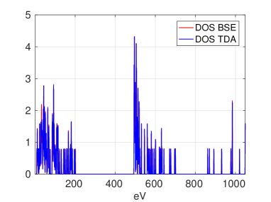
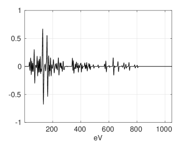
Figure 2.2: DOS for H₂O, $\eta=0.5$: exact BSE vs. TDA on the full spectrum (left), the absolute error (right).

It was numerically demonstrated in [6] that the spectrum of the TDA model provides a good approximation to the spectrum of the full BSE Hamiltonian. The difference between the two is on the order of $10^{-2}$ for molecules of moderate size.

Figure 2.2, left, compares the DOS for the H₂O molecule calculated via the eigenvalues of the full BSE Hamiltonian and those of the TDA approximation, while on the right we display the corresponding maximum error.

Figure 2.3, left, compares the same DOS calculations but zoomed on the first compact energy interval $[0,40]$ eV. The red curve corresponds to the full BSE data, and the blue one represents the TDA case. The figure on the right displays the corresponding maximum error.

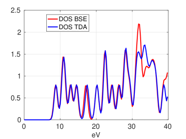
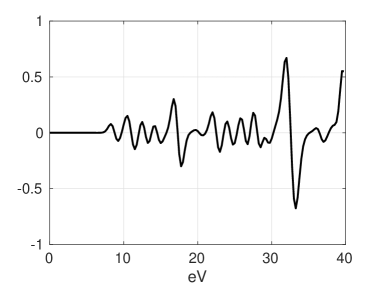
Figure 2.3: DOS for H₂O on the energy sub-interval $[0,40]$: exact BSE vs. TDA (left), and the error (right).

Figure 2.4, left, represents the DOS for H₂O computed by using the exact TDA spectrum (blue) and its approximation based on a simplified model obtained via low-rank approximation to $A$ (red), while the right figure shows the relative error.

Figures 2.5 presents the DOS for H₁₆ (left) and H₃₂ (right) chains of Hydrogen atoms. We observe the essential similarity in the shapes (only the amplitude is changing) which is apparently a consequence of quasi-periodicity of the system.

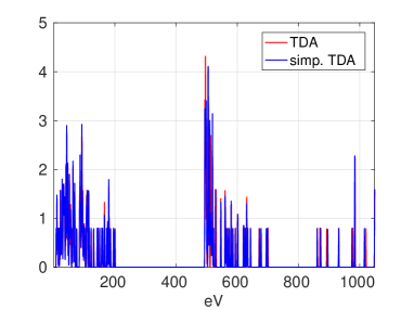
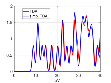
Figure 2.4: DOS for H₂O. Exact TDA vs. simplified TDA (left), zoom of the small spectral interval (right).

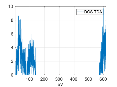
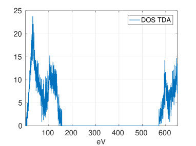
Figure 2.5: DOS for H₁₆ (left) and H₃₂ (right) chains of Hydrogen atoms.

The rank-structured approach to calculation of the molecular absorption spectrum in the case of full BSE is sketched in §5. This topic will be addressed elsewhere.

2.3 General description of the existing computational schemes

One of the commonly used approaches to the numerical approximation of both functions $g_{\eta}(t)$ and $L_{\eta}(t)$ is based on the construction of certain polynomial or fractional polynomial interpolants whose evaluation at each sampling point $t_{k}$ requires the solution of a large linear system with the BSE/TDA matrix, i.e., remains expensive.

In the case of Lorentzian broadening (2.7) the regularized DOS takes the form

$$\phi(t)\approx\phi_{\eta}(t):=\frac{1}{n\pi}\sum\limits_{j=1}^{n}\mbox{Im}\left(\frac{1}{(t-\lambda_{j})-i\eta}\right)=\frac{1}{n\pi}\mbox{Im}\,\mbox{Trace}[(tI-A-i\eta I)^{-1}].$$ (2.8)

To keep real-valued arithmetics, likewise, we can write the latter in the form

$$\phi_{\eta}(t):=\frac{1}{n\pi}\sum\limits_{j=1}^{n}\frac{\eta}{(t-\lambda_{j})^{2}+\eta^{2}}=\frac{1}{n\pi}\mbox{Trace}[((tI-A)^{2}+\eta^{2}I)^{-1}].$$ (2.9)

In both cases the task of computing the approximate DOS $\phi_{\eta}(t)$ reduces to approximating the trace of the matrix resolvent

$$(tI-A-i\eta I)^{-1}\quad\mbox{or}\quad((tI-A)^{2}+\eta^{2}I)^{-1}.$$

Here, the price to pay for real-valued arithmetics is to address the more complicated low-rank structure in $(tI-A)^{2}$.

The traditional approach [25] to approximately computing the traces of the matrix-valued analytic function $f(A)$ reduces this task to the estimation of the mean of $v_{m}^{T}f(A)v_{m}$ over a sequence of random vectors $v_{m}$, $m=1,\ldots,m_{r}$, satisfying certain condition (see [25], Theorem 3.1). That is, $\mbox{Trace}[f(A)]$ is approximated by

$$\mbox{Trace}[f(A)]\approx\frac{1}{m_{r}}\sum\limits_{m=1}^{m_{r}}v_{m}^{T}f(A)v_{m}.$$ (2.10)

The calculation of (2.10) for

$$f_{1}(A)=(tI-A-i\eta I)^{-1}\quad\mbox{or}\quad f_{2}(A)=((tI-A)^{2}+\eta^{2}I)^{-1}$$ (2.11)

reduces to solving linear systems in the form of

$$(tI-i\eta I-A)x=v_{m}\quad\mbox{for}\quad m=1,\ldots,m_{r},$$ (2.12)

or

$$(\eta^{2}I+(tI-A)^{2})x=v_{m}\quad\mbox{for}\quad m=1,\ldots,m_{r}.$$ (2.13)

These linear systems need to be solved for many target points $t=t_{k}\in[a,b]$ in the course of a chosen interpolation scheme.

In the case of rank-structured matrices $A$, the solution of equations (2.12) or (2.13) can be implemented with a lower cost. However, even in this favorable situation one requires a relatively large number $m_{r}$ of stochastic realizations to obtain satisfactory mean value approximation. The convergence rate is expected to be on the order of $O(1/\sqrt{m_{r}})$. On the other hand, with the limited number of interpolation points, the polynomial type of interpolation schemes applied to highly non-regular shapes as shown, say, in Figure 2.4 (left), can only provide limited resolution and is unlikely to reveal spectral gaps and many local peaks of interest.

3 Fast evaluation of DOS for rank-structured matrices

3.1 DOS by the trace of rank-structured matrix inverse

In what follows, we propose an approach that is based on evaluating the trace term in (2.8) directly (without stochastic sampling). This approach relies on the following two techniques:

• using the low-rank BSE matrix structure as in [6], which allows for each fixed $t\in[0,a]$ the direct matrix inversion and computation of the respective traces,

• the low-rank QTT tensor interpolation of the function $L_{\eta}(t)$ sampled on a fine uniform grid $\{t_{1},\ldots,t_{M}\}$ in the whole spectral interval $[0,a]$ or on some subinterval of $[0,a]$.

For the class of block-diagonal plus low-rank matrices arising in the reduced model approach for BSE problem [6, 3], we have (see §2.1 for more details)

$$A=E+PQ^{T},\quad\mbox{with}\quad P,Q\in\mathbb{R}^{n\times R},\quad E=\mbox{blockdiag}\{B_{0},D_{0}\},$$ (3.1)

where the rank parameter $R$ is small compared to $n$, the full $n_{B}\times n_{B}$ matrix block $B_{0}$ is of size $n_{B}=O(n^{\alpha})$, $0<\alpha<1$, and $D_{0}$ is a diagonal matrix of size $n-n_{B}$.

Notice that even in the case of structured matrices in (3.1) the traditional approach by (2.10) leads to a sequence of linear systems (2.12) to be solved many times in the course of stochastic sampling, for each of many interpolation points $t\in[0,a]$.

In our approach, for the class of rank-structured matrices (3.1), we propose to avoid stochastic sampling in (2.10) by introducing a direct scheme that allows us to evaluate the trace of matrices $f_{1}(A)$ or $f_{2}(A)$ defined in (2.11), corresponding to the matrix resolvent in (2.8) and (2.9), respectively, by one-step straightforward matrix calculation.

To that end, let us first construct the reduced-model approximation to the matrix inverse $A^{-1}$ for the matrix in (3.1), where the block-diagonal part $E(t)=\mbox{blockdiag}\{B(t),D(t)\}$ corresponds to the case of (2.8), i.e.,

$$B(t)=tI_{B}-i\eta I_{B}+B_{0},\quad D(t)=tI_{D}-i\eta I_{D}+D_{0}.$$ (3.2)

Here $B_{0}$ and $D_{0}$ denote the corresponding matrix blocks in the representation of the diagonal block $A$ in the initial BSE matrix, see (3.1), and $I_{B},I_{D}$ denote the identity matrices corresponding to the respective index subsets. For the ease of exposition, we further assume that the matrix size of the block $B$ in (3.2) is bounded by $n_{B}=O(n^{\alpha})$ with $\alpha\leq 1/3$. This assumption on the block size ensures the linear complexity scaling of our algorithm in the matrix size $n$.

In what follows, we use the notion ${\bf 1}_{m}$ for a length-$m$ vector of all ones, and $\odot$ for the Hadamard product of matrices.

The following result asserts that the cost of trace calculations is estimated to be $O(nR)$.

Theorem 3.1

Let the matrix family $A=A(t)$, $t\in[0,a]$, be given by (3.1), with

$$E=E(t)=\mathrm{blockdiag}\{B(t),D(t)\},$$

where $B(t),D(t)$ are defined in (3.2). Then the trace of the matrix inverse $A(t)^{-1}$ can be calculated explicitly by

$$\mathrm{trace}[A(t)^{-1}]=\mathrm{trace}[B(t)^{-1}]+\mathrm{trace}[D(t)^{-1}]-{\bf 1}_{n}^{T}({U(t)}\odot{V(t)}){\bf 1}_{R},$$

where ${U(t)}=E(t)^{-1}PK(t)^{-1}\in\mathbb{R}^{n\times R}$, ${V(t)}=E(t)^{-1}Q\in\mathbb{R}^{n\times R}$, and

$$K(t)=I_{R}+Q^{T}E(t)^{-1}(t)P$$

is a small $R\times R$ matrix. For fixed $t\in[0,a]$, assume that $n_{B}=O(n^{\alpha})$ with $\alpha\leq 1/3$, then the numerical cost is estimated by $O(nR^{2})$.

Proof. The analysis relies on the particular structure of the matrix blocks. Indeed, we use the direct trace representation for both rank-$R$ and block-diagonal matrices. Our argument is based on the observation that the trace of a rank-$R$ matrix $U(t)V(t)^{T}$, where $U(t),V(t)\in\mathbb{R}^{n\times R}$, $U(t)=[{\bf u}_{1},\ldots,{\bf u}_{R}]$, $V(t)=[{\bf v}_{1},\ldots,{\bf v}_{R}]$, ${\bf u}_{k},{\bf v}_{k}\in\mathbb{R}^{n}$, can be calculated in terms of skeleton vectors by

$$\mbox{trace}[U(t)V(t)^{T}]=\sum_{k=1}^{R}\langle{\bf u}_{k},{\bf v}_{k}\rangle={\bf 1}_{n}^{T}(U(t)\odot V(t)){\bf 1}_{R},$$

at the expense $O(Rn)$. For fixed $t$, define the rank-$R$ matrices by

$$U(t)=E(t)^{-1}PK(t)^{-1},\quad V(t)=E(t)^{-1}Q,$$

then the Sherman-Morrison scheme leads to the representation, see [3],

$$A(t)^{-1}=\mbox{blockdiag}\{B(t)^{-1},D(t)^{-1}\}-E(t)^{-1}PK(t)^{-1}Q^{T}E(t)^{-1},$$

where the last term simplifies to

$$E(t)^{-1}PK(t)^{-1}Q^{T}E(t)^{-1}=U(t)V(t)^{T}.$$

Now we apply the above formula for the trace of a rank-$R$ matrix to obtain the desired representation.

The complexity estimate follows taking into account the bound on the size of matrix block $B$. Indeed, forming $U(t)$ involves solving the linear system $P_{1}(t)=U(t)K(t)$, for $U(t)$, where $P_{1}(t)$ is the pre-computed $E(t)^{-1}P$, which can be computed by assumptions at the cost $O(nR)$. Here $P_{1}(t)$ would be re-used to compute $K(t)$ itself, and thus stored. The cost for solving this system of equations is $2/3R^{3}$ (LU factorization of $K(t)$), plus $2nR^{2}$ for backward/forward solves. This completes the proof.   

The above representation has to be applied many times for calculating the trace of $E(t_{m})^{-1}PK(t_{m})^{-1}Q^{T}E(t_{m})^{-1}$ at each fixed interpolating point $t_{m}$, $m=1,\ldots,M$.

Here, we notice that the price to pay for the real arithmetics in equation (2.13) is that we compute with squared matrices which, however, do not increase the asymptotic complexity since there is no increase of the rank in the rank-structured representation of the system matrix, see the following Theorem 3.2. In our applications we do not expect a loss of numerical stability of the algorithm since the condition numbers of $E(t)$ are moderate. In what follows we denote by $[U,V]$ the concatenation of two matrices of compatible size.

Theorem 3.2

Given matrix $S=(tI-A)^{2}+\eta^{2}I$, where $A$ is defined by (3.1), then the trace of the real-valued matrix resolvent $S^{-1}(t)$ can be calculated explicitly by

$$\mathrm{trace}[S^{-1}]=\mathrm{trace}[E_{0}^{-1}]-{\bf 1}_{n}^{T}(\overline{U}\odot\overline{V}){\bf 1}_{2R},$$ (3.3)

with $\overline{U}=E_{0}^{-1}\overline{P}K^{-1}\in\mathbb{R}^{n\times 2R}$, and $\overline{V}=E_{0}^{-1}\overline{Q}\in\mathbb{R}^{n\times 2R}$, where the real-valued block-diagonal matrix $E_{0}$ is given by

$$E_{0}(t)=\eta^{2}I+t^{2}I-2tE+E^{2}=(\eta^{2}+t^{2})I+\mathrm{blockdiag}[B^{2}-2tB,D^{2}-2tD],$$

and the rank-$2R$ matrices $\overline{P},\overline{Q}$ are represented via concatenation

$$\overline{P}=[-2tQ+EQ+QE+Q(Q^{T}Q),Q]\in\mathbb{R}^{n\times 2R},\quad\overline{Q}=[Q,EQ]\in\mathbb{R}^{n\times 2R},$$

such that the small core matrix $K(t)\in\mathbb{R}^{2R\times 2R}$ takes the form $K(t)=I_{R}+\overline{Q}^{T}E_{0}^{-1}(t)\overline{P}$.

Assume that $n_{B}=O(n^{\alpha})$ with $\alpha\leq 1/3$, then the numerical cost is estimated by $O(nR^{2})$ up to a low order term.

Proof. Indeed, given the block-diagonal plus low-rank matrix $A$ in the form (3.1), we obtain

$$S=(tI-A)^{2}+\eta^{2}I=E_{0}+\overline{P}\,\overline{Q}^{T},$$

where the block-diagonal matrix $E_{0}$ and the rank-$2R$ matrix $\overline{P}\,\overline{Q}^{T}$ are defined as above. Applying the Sherman-Morrison scheme as above to the block-diagonal plus rank-$2R$ matrix structure in $S$, the representation result follows. Now we take into account that

$$\mathrm{trace}[E_{0}^{-1}]=\mathrm{trace}[(B^{2}-2tB)^{-1}]+\mathrm{trace}[(D^{2}-2tD)^{-1}],$$

then the restriction on the size of the block $B$ proves the complexity bound similar to the argument in the proof of the previous theorem.   

Based on Theorems 3.1 and 3.2, the calculations in item (A) can be implemented efficiently in both complex and real arithmetics. The following numerics demonstrates the efficiency of the DOS calculation for the rank-structured TDA matrix implemented in real arithmetics as described by (3.3) in Theorem 3.2.

Molecule	H2O	NH3	H2O2	N2H4	C2H5OH	C2H5 NO2	C3H7 NO2
$n=N_{ov}$	$180$	$215$	$531$	$657$	$1430$	$3000$	$4488$
Rank $R$	$36$	$30$	$68$	$54$	$74$	$129$	$147$
Total time $T$ (s)	$6.7$	$7.7$	$33$	$47$	$219$	$1084$	$2223$
Scaled time $T/R^{2}$ (s)	$0.005$	$0.008$	$0.007$	$0.017$	$0.041$	$0.065$	$0.103$

Table 3.1: Scaled times for the Algorithm in Theorem 3.2.

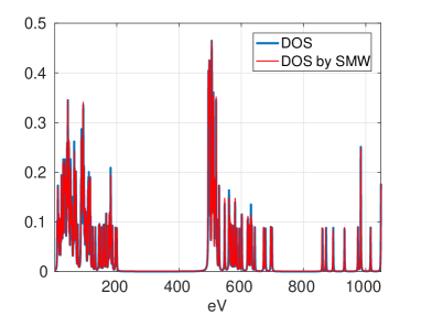
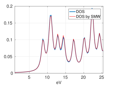
Figure 3.1: Left: DOS for H₂O vs. its recovering by using the trace of matrix resolvents; Right: zoom on the small energy interval.

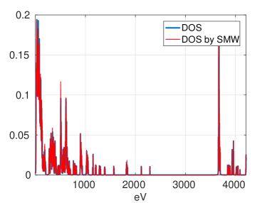
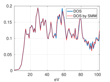
Figure 3.2: Left: DOS for Ethanol molecule vs. its recovering by using the trace of matrix resolvents; Right: zoom on the small energy interval.

Figures 3.1 and 3.2 demonstrate that using only the structure-based trace representation (3.3) in Theorem 3.2, we obtain the approximation which resolves perfectly the DOS function (for the examples of H₂O and Ethanol molecules). The exact DOS is shown by the blue line, while the results of structure-based DOS calculation is indicated by the red line (we use the acronym “SMW” for the Sherman-Morrison-Woodbury scheme).

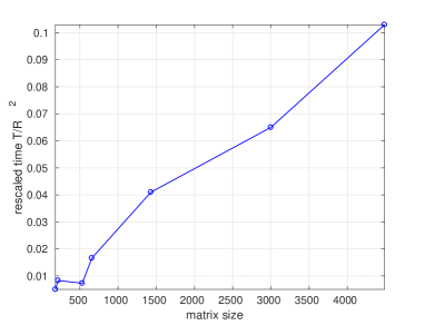
Figure 3.3: Algorithm in Theorem 3.2: the rescaled CPU time $T/R^{2}$ versus $n$.

Figure 3.3 shows the rescaled CPU time, i.e. $T/R^{2}$, where $T$ denotes the total CPU time for computing the DOS by the algorithm implied by Theorem 3.2. This demonstrates almost linear complexity scaling of the algorithm in $n$, $O(R^{2}n)$. We applied the algorithm to molecules of different system size $n$ (i.e. the size of TDA matrix) varying from $n=180$ till $n=4488$ (see Table 3.1 for more details). In all cases the $N$-point representation grid with fixed $N=2^{14}$ was used.

We conclude that the algorithm based on representation (3.3) demonstrates the perfect resolution of the DOS function at linear complexity in the system size which allows to treat large molecules.

The approach in item (B) requires fast trace calculations for many different values of parameter $t_{m}\in\tau=\{t_{1},\ldots,t_{M}\}\subset[0,a]$ in the matrix resolvent. Finer resolution of the spectrum for large molecular systems leads to a considerable increase of the number of samples $M$ that is practically equal to the grid size, $M=N$. Hence, the total cost $O(MnR^{2})$ may become prohibitively expensive since the trace computation for each fixed value of $t_{m}$ still requires complicated matrix operations (see Theorems 3.1 and 3.2).

3.2 Calculating multiple traces of $A^{-1}$ with lower cost

In this section, we describe a further enhancement scheme for fast multiple calculation of traces on the large set of interpolation points. We outline how it is possible to reduce the complexity of these calculations (reduced model) by using a certain smoothness in $t$ in the parametric matrix resolvent by introducing the low rank approximation of the large $n^{2}\times M$ matrix

$$\mathbb{E}(t)=[E(t_{1})^{-1},\ldots,E(t_{M})^{-1}]\quad\mbox{and}\quad\mathbb{K}(t)=[K(t_{1})^{-1},\ldots,K(t_{M})^{-1}]\in\mathbb{R}^{R^{2}\times M}$$

obtained by concatenation of vectorized matrices $E(t_{m})^{-1}$ and $K(t_{m})^{-1}$, $m=1,\ldots,M$, respectively. The idea is that

$$E(t)^{-1}=\mbox{blockdiag}[P(t)^{-1},D(t)^{-1}]$$

defines an analytic matrix family on the spectral interval $t\in[0,a]$, and so is the family of core matrices $\{K^{-1}(t)\}$. This favorable property allows the model reduction via low rank approximation of the matrix families $\mathbb{E}(t)$ and $\mathbb{K}(t)$, $t\in\tau$. Suppose that the representations

$$K(t)^{-1}=\sum\limits_{k=1}^{R_{K}}c_{k}(t)K_{k}$$

and

$$E(t)^{-1}=\mbox{blockdiag}[P(t)^{-1},D(t)^{-1}]=\sum\limits_{m=1}^{R_{E}}p_{m}(t)E_{m}$$

are precomputed (this is an additional low-rank approximation procedure which separates the parameter $t$), where $E_{m}=\mbox{blockdiag}[P_{m},D_{m}]\in\mathbb{R}^{n\times n}$ and $K_{k}\in\mathbb{R}^{R\times R}$ do not depend on $t$, and $E_{m}$ inherits the block-diagonal structure that $E(t)^{-1}$ obeys.

We take into account that $Q$ does not depend on $t$, and plug the above decompositions in the main trace-term to obtain

$$\mbox{Trace}[E^{-1}QK^{-1}Q^{T}E^{-1}]=\mbox{Trace}\left[\sum\limits_{m=1}^{R_{E}}p_{m}(t)E_{m}\,Q\,(\sum\limits_{k=1}^{R_{K}}c_{k}(t)K_{k})\,Q\sum\limits_{m^{\prime}=1}^{R_{E}}p_{m^{\prime}}(t)E_{m^{\prime}}\right].$$

Now it follows that

$$\mbox{Trace}[E^{-1}QK^{-1}Q^{T}E^{-1}]=\sum\limits_{m=1}^{R_{E}}p_{m}(t)\sum\limits_{k=1}^{R_{K}}c_{k}(t)\sum\limits_{m^{\prime}=1}^{R_{E}}p_{m^{\prime}}(t)\mbox{Trace}[E_{m}QK_{k}QE_{m^{\prime}}],$$

where $K_{k}\in\mathbb{R}^{R\times R}$ is a small matrix, $Q\in\mathbb{R}^{n\times R}$, $E_{m}=\mbox{blockdiag}[P_{m},D_{m}]$ with diagonal $D_{m}$ and the full $n_{P}\times n_{P}$ matrix $P_{m}$, such that $n_{P}=O({n}^{\alpha})$.

With these prerequisites, we pre-compute a set of ”time-independent” traces

$$T_{mkm^{\prime}}=\mbox{Trace}[E_{m}QK_{k}QE_{m^{\prime}}],\quad m,m^{\prime}=1,\ldots,R_{E},\;\;k=1,\ldots,R_{K},$$ (3.4)

and store the $R_{E}^{2}R_{K}$ numbers $T_{mkm^{\prime}}$ to obtain the cheap representation of the trace in terms of only a scalar sum,

$$\mbox{Trace}[E^{-1}QK^{-1}Q^{T}E^{-1}](t)=\sum\limits_{m=1}^{R_{E}}\sum\limits_{k=1}^{R_{K}}\sum\limits_{m^{\prime}=1}^{R_{E}}p_{m}(t)c_{k}(t)p_{m^{\prime}}(t)T_{mkm^{\prime}}.$$

The cost of precomputing each trace-value $T_{mkm^{\prime}}$ is estimated by $O(n^{3\alpha}R^{2})$ as proven by Theorem 3.1, while the number of coefficients to be stored is about $O(R_{E}^{2}R_{K})$ and it is expected to be small or moderate. With these data at hand, the evaluation of the required trace for the particular $t_{\nu}\in\tau$ takes $O(R_{E}^{2}R_{K})$ scalar operations independently on $n$.

Notice that the computations in (3.4) are intrinsically parallel, which can be exploited on modern computing hardware using multi-threading or distributed computing.

4 QTT approximation of DOS

In what follows, we discuss the QTT approximation of the DOS. We also describe a tensor based heuristic QTT approximation of the DOS by using only an incomplete set of sampling points, i.e., QTT representation by adaptive cross approximation (ACA) [30, 36]. Furthermore, we derive the upper bound on the QTT ranks of the DOS by the Gaussians broadening.

4.1 Quantized-TT approximation of function related vectors

In the case of large vector size $N$, the number of representation parameters for the corresponding high-order QTT tensor can be reduced to the logarithmic scaling $\mathcal{O}(\log N)$, which allows the QTT tensor interpolation of the target $N$-vector by using only $\mathcal{O}(\log N)\ll N$ entries, which are chosen adaptively by the heuristic ACA algorithm [30, 36]. The accuracy of this kind of “approximate interpolation” is controlled by the $\varepsilon$-truncation of the QTT rank parameters. In the present paper, we apply this approximation technique to long $N$-vectors representing the DOS sampled over the fine representation grid $\Omega_{h}$.

The QTT-type approximation of an $N$-vector with $N=q^{d^{\prime}}$, $d^{\prime}\in\mathbb{N}$, $q=2,3,...$, is defined as the tensor decomposition (approximation) in the TT or canonical format applied to a tensor obtained by the folding (reshaping) of the initial vector to a $d^{\prime}$-dimensional $q\times\cdots\times q$ data array. The latter is thought of as an element of the multi-dimensional quantized tensor space $\mathbb{Q}_{{q},d^{\prime}}=\bigotimes_{j=1}^{d^{\prime}}\mathbb{K}^{q}$, $\mathbb{K}\in\{\mathbb{R},\mathbb{C}\}$, and $d^{\prime}$ is the auxiliary dimension (virtual, in contrary to the real space dimension $d$) parameter that measures the depth of the quantization transform. A vector ${\bf x}=[x_{i}]_{i\in I}\in\mathbb{R}^{N},$ is reshaped to its multi-dimensional quantized image in $\mathbb{Q}_{q,d^{\prime}}$ by $q$-adic folding,

$$\mathcal{F}_{q,d^{\prime}}:{{\bf x}\to\bf{X}}=[x({\bf j})]\in\mathbb{Q}_{q,d^{\prime}},\quad{\bf j}=\{j_{1},\ldots,j_{d^{\prime}}\},$$

with $j_{\nu}\in\{1,\ldots,q\}$ for $\nu=1,\ldots,d^{\prime}$. Here, for fixed $i$, we have $x({\bf j}):=x_{i}$, and $j_{\nu}=j_{\nu}(i)$ is defined via $q$-coding, $j_{\nu}-1=C_{-1+\nu},$ such that the coefficients $C_{-1+\nu}$ are found from the $q$-adic representation of $i-1$ (binary coding for $q=2$),

$$i-1=C_{0}+C_{1}q^{1}+\cdots+C_{d^{\prime}-1}q^{d^{\prime}-1}\equiv\sum\limits_{\nu=1}^{d^{\prime}}(j_{\nu}-1)q^{\nu-1}.$$

Assuming that for the rank-${\bf r}$ TT approximation of the quantized image ${\bf{X}}$ there holds $r_{k}\leq r$, $k=1,\ldots,d^{\prime}$, the complexity of this representation for the tensor ${\bf{X}}$ reduces to the logarithmic scale

$$qr^{2}\log_{q}N\ll N.$$

The computational gain of the QTT approximation is justified by the perfect rank decomposition proven in [23] for a wide class of function-related tensors obtained by sampling the corresponding functions over a uniform or properly refined grid. This class of functions includes complex exponentials, trigonometric functions, polynomials and Chebyshev polynomials, as well as wavelet basis functions. We refer to [11, 29, 19, 24] for further results on QTT approximation of functional vectors and various applications.

In estimating the numerical complexity we use the average QTT rank further denoted by $r_{qtt}$ calculated as follows,

$$r_{qtt}=\sqrt{\frac{1}{d-1}\sum\limits^{d-1}_{k=1}r_{k}^{2}},$$ (4.1)

where the QTT ranks $r_{k}$ are the TT ranks of the quantized image ${\bf X}$ of a vector.

As an example we present the basic results on the rank-$1$ (resp. rank-$2$) QTT representation (with $q=2$) of the exponential (resp. trigonometric) vectors [23]. For given $N=2^{d^{\prime}}$, and $z\in\mathbb{C}$, the exponential $N$-vector, ${\bf z}:=\{z_{n}=z^{n-1}\}_{n=1}^{N},$ can be reshaped by the dyadic folding to the rank-$1$, $2^{\otimes d^{\prime}}$-tensor,

$$\mathcal{F}_{2,d^{\prime}}:{\bf z}\mapsto{\textbf{Z}}=\otimes_{p=1}^{d^{\prime}}[1\;z^{2^{p-1}}]^{T}\in\mathbb{Q}_{{2},d^{\prime}}.$$ (4.2)

The number of representation parameters specifying the QTT image is reduced dramatically from $N$ to $2\log_{2}N$.

The trigonometric $N$-vector, ${\bf t}=\Im m({\bf z}):=\{t_{n}=\sin(\omega(n-1))\}_{n=1}^{N},\quad\omega\in\mathbb{R},$ can be reshaped by the successive dyadic folding

$$\mathcal{F}_{2,d^{\prime}}:{\bf t}\mapsto{\textbf{T}}\in\mathbb{Q}_{{2},d^{\prime}},$$

to the $2^{\otimes d^{\prime}}$-tensor T, which has both the canonical and the QTT-rank equal to $2$, in the complex and real arithmetics, respectively.

The explicit rank-$2$ QTT-representation of the single $\sin$-vector in $\{0,1\}^{\otimes d^{\prime}}$ (see [12, 29]) with $k_{p}=2^{p-1}i_{p}$, $i_{p}\in\{0,1\}$, reads

$${\bf t}\mapsto{\textbf{T}}=\Im m({\textbf{Z}})=[\sin\,\omega k_{1}\cos\,\omega k_{1}]\otimes_{p=2}^{d^{\prime}-1}\left[\begin{array}[]{c c}\cos\,\omega k_{p}&-\sin\,\omega k_{p}\\ \sin\,\omega k_{p}&\cos\,\omega k_{p}\end{array}\right]\otimes\left[\begin{array}[]{c}\cos\,\omega k_{d^{\prime}}\\ \sin\,\omega k_{d^{\prime}}\end{array}\right].$$

The number of representation parameters is $8(d^{\prime}-1)$. A more detailed discussion of the QTT approximation for function related vectors can be found in [23, 24].

In cases when the exact low-rank QTT representation is not known, an $\varepsilon$-approximation in the QTT format can be computed by using the standard TT multi-linear approximation tools [28]. As a first illustration, we consider the QTT approximation of the DOS for the 1D finite difference Laplacian operator in $[0,\pi]$ with Dirichlet boundary conditions, $A=-\mbox{tridiag}\{1,-2,1\}\in\mathbb{R}^{n\times n}$, discretized on the uniform grid of size $h=\pi/(n+1)$ with $n=2047$. The corresponding eigenvalues are given by

$$\lambda_{k}=4\sin^{2}(\frac{\pi k}{2n}),\quad k=1,\ldots,n.$$

Figure 4.1 represents the Lorentzian-DOS and the corresponding approximation error for its QTT $\varepsilon$-interpolant with $r_{qtt}=5$, computed on the representation grid of size $N=2^{14}$.

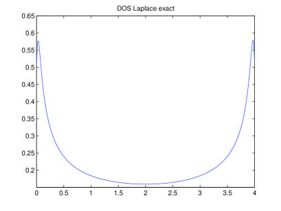
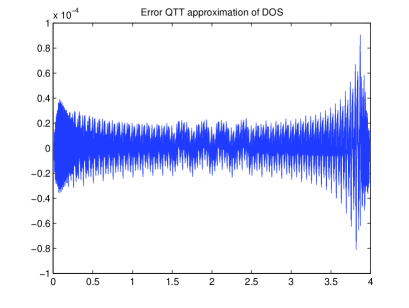
Figure 4.1: DOS for Laplacian (left), and its QTT approximation with $r_{qtt}=5$ (right).

In this paper we apply the QTT approximation method to the DOS regularized by Gaussians or Lorentzians and sampled on a fine representation grid of size $N=2^{d^{\prime}}$. The QTT approximant can be viewed as the rank structured $\varepsilon$-interpolant to the highly non-regular function $\phi_{\eta}$ regularizing the exact DOS. In this case the application of traditional polynomial or trigonometric type interpolation is inefficient.

The QTT approach provides a good approximation to $\phi_{\eta}$ on the whole spectral interval and requires only a moderate number of representation parameters $r_{qtt}^{2}\log N\ll N$, where the average QTT rank $r_{qtt}$, see (4.1) is a small rank parameter adaptively depending on the truncation error $\epsilon>0$.

4.2 QTT approximation to DOS via Lorentzians: proof of concept

In this section we demonstrate the efficiency of the QTT approximation applied to the DOS via both Gaussian and Lorentzian blurring. We verify by various numerical experiments that the low-rank QTT approximant resolves perfectly the exact DOS.

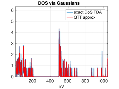
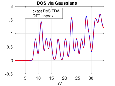
Figure 4.2: DOS (in eV) for the H₂O molecule via Gaussians (left), and zoom on the left most part of the spectrum. Here $r_{QTT}=9.4$, $\eta=0.4$

In the following numerical examples, we use a sampling vector defined on a grid of size $N\approx 2^{14}$. We set the QTT truncation error to $\epsilon_{QTT}=0.04$, if not explicitly indicated. For ease of interpretation, we set the pre-factor in (2.4) to $1$. It is worth noting that the QTT-approximation scheme is applied to the full TDA spectrum. Our results demonstrate that it renders good resolution in the whole range of energies (in eV) including large ”zero gaps”.

Figure 4.2, left, represents the TDA DOS (blue line) for H₂O computed by Gaussian blurring with the parameter $\eta=0.4$, and the corresponding rank-$9.4$ QTT tensor approximation (red line) to the discretized function $\phi_{\eta}(t)$. For this example, the number of eigenvalues is given by $n=N_{BSE}/2=180$. Figure 4.2, right, provides a zoom of the corresponding DOS and its QTT approximant within the small energy interval $[0,40]$eV.

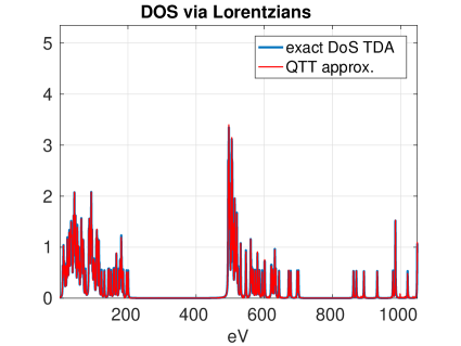
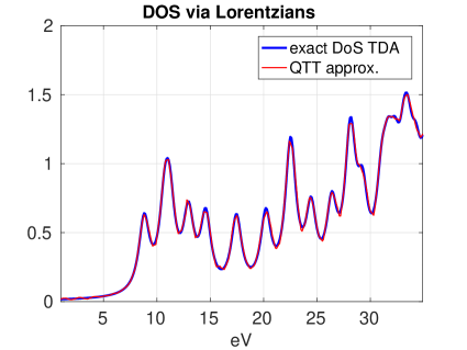
Figure 4.3: DOS for H₂O molecule via Lorentzians (blue) and its QTT approximation (red) (left). Zoom on the left most part of the spectrum (right). $\varepsilon$=0.04, $r_{QTT}=10.5$.

Figure 4.3 demonstrates the resolution of the QTT approximation to the DOS via the Lorentzian blurring indicating similar QTT-ranks as in the case of the Gaussians regularization.

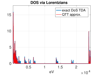
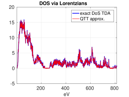
Figure 4.4: DOS for Glycine amino acid via Lorentzians (blue) and its QTT approximation (red), left; (left). Right: zoom of the first part of the spectrum. $\varepsilon$=0.04, $r_{QTT}=16$.

Figure 4.4 (Lorentzian blurring) represents similar data, but for the large Glycine amino acid with $n=N_{TDA}=3000$. It is worth noting that the average QTT rank of $\phi_{\eta}(t)$ sampled on $N=2^{14}$ grid points is about $r_{QTT}=16$, ($\epsilon_{QTT}=0.04$) though the number of eigenvalues $n$ in this case is about $20$ times larger than for the water molecule. This means that for a fixed $\eta$, the QTT-rank remains rather modest relative to the molecular size. This observation confirms Theorem 4.1 in Section 4.4.

A comparison of Figures 4.2 and 4.3 indicates that the Lorentzian based DOS blurring is slightly smoother than Gaussian blurring. The moderate size of the QTT ranks in Figures 4.3 and 4.4 clearly shows the potentials of the QTT $\varepsilon$-interpolation for modeling the DOS of large lattice type clusters.

We observe several gaps in the spectral densities, see Figure 4.2, 4.3 and 4.4 indicating that polynomial, rational or trigonometric interpolation can be applied only to some energy sub-intervals, but not in the whole interval $[a,b]$. Remarkably, the QTT approximant resolves well the DOS function in the whole energy interval including nearly zero values within the spectral gaps (hardly possible for polynomial/rational based interpolation).

4.3 Numerics for the QTT interpolation to the DOS function

In the previous section we demonstrated that the QTT tensor approximation provides good resolution for the DOS function calculated for a number of molecules. In what follows, we describe a tensor based heuristic QTT approximation of the DOS by using only an incomplete set of sampling points, i.e., QTT representation by adaptive cross approximation (ACA) [30, 36]. This allows us to recover the spectral density in controllable accuracy with $M$ interpolation points, where $M$ asymptotically scales logarithmically in the grid size $N$. This heuristic approach can be viewed as a kind of “adaptive QTT $\varepsilon$-interpolation”. In particular, we show by numerical experiments that the low-rank QTT adaptive cross interpolation provides a good resolution of the target DOS with the number of functional calls that asymptotically scales logarithmically, $O(\log N)$, in the size $N$ of the representation grid.

In the case of large $N$, the QTT interpolant can be computed by the ACA tensor approximation procedure (see [30, 36] for the detailed description) that, in general, does not require the full set of functional values over the $N$-grid. In the case of large $N$ this beneficial feature allows to compute the QTT approximation by requiring less than $N$ computationally expensive functional evaluations of $\phi_{\eta}(t)$.

The QTT interpolation via ACA tensor approximation serves to recover the representation parameters of the QTT tensor approximant and normally requires about

$$M=C_{s}r_{qtt}^{2}\log_{2}N$$ (4.3)

samples of the target $N$-vector with a small pre-factor $C_{s}$, usually satisfying $C_{s}\leq 10$, that is independent of the fine interpolation grid size $N=2^{d^{\prime}}$, see, for example, [22]. This cost estimate seems promising in the perspective of extended or lattice type molecular systems, requiring large spectral intervals and, as a result, a large interpolation grid of size $N$. Here the QTT rank parameter $r_{qtt}$ naturally depends on the required truncation threshold $\varepsilon>0$, characterizing the $L_{2}$-error between the exact DOS and its QTT interpolant. The QTT tensor interpolation reduces the number of functional calls, i.e., $M<N$, if the QTT rank parameters (or threshold $\varepsilon>0$) are chosen to satisfy the condition

$$M=C_{s}r_{qtt}^{2}\log_{2}N\leq N.$$

The expression on the left-hand side provides a rather accurate estimate on the number of functional evaluations.

To complete this discussion, we present numerical tests for the low-rank QTT tensor interpolation applied to the long vector discretizing the Lorentzian-DOS on a fine representation grid of size $N=2^{d^{\prime}}$.

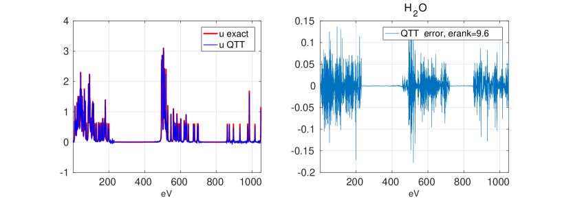
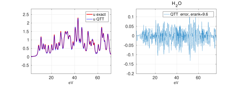
Figure 4.5: QTT ACA interpolation of the DOS for H₂O (top) and zoom in to a small spectral interval (bottom).

Figure 4.5 represents the results of the QTT interpolating approximation to the discretized DOS function (H₂O molecule). We use the QTT cross approximation algorithm based on [23, 30, 36, 29] and implemented in the MATLAB TT-toolbox (https://github.com/oseledets/TT-Toolbox). Here we set $\varepsilon=0.08$, $\eta=0.1$ and $N=2^{14}$, providing $r_{QTT}=9.8$. The top two figures display the results on the whole spectral interval, while the bottom figures show the zoom of the same data in the small spectral interval $[0,55]$eV.

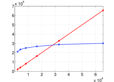
Figure 4.6: DOS for H₂O via Lorentzians: the number of functional calls for QTT cross approximation (blue) vs. the full grid size $N$.

Figure 4.6 illustrates the logarithmic increase in the number of samples required for the QTT interpolation of the DOS (for the H₂O molecule) represented on the grid of size $N=2^{d^{\prime}}$, where $d^{\prime}=11,12,\ldots,16$, provided that the rank truncation threshold is chosen by $\epsilon=0.05$ and the regularization parameter is $\eta=0.2$. In this example, the effective pre-factor in (4.3) is estimated by $C_{s}\leq 10$. This pre-factor characterizes the average number of samples required for the recovery of each of the $r_{qtt}^{2}\log N$ representation parameters involved in the QTT tensor ansatz.

We observe that the QTT tensor interpolant recovers the exact DOS with a high precision. The logarithmic asymptotic complexity scaling $O(\log N)$ (i.e. the number of functional calls required for the QTT tensor interpolation) vs. the grid size $N$ can be observed in Figure 4.6 (blue line).

4.4 Upper bounds on the QTT ranks of DOS

In this section we analyze the upper bounds on the QTT ranks of the discretized DOS obtained by Gaussian broadening. Our numerical tests indicate that Lorentzian blurring leads to a similar QTT rank compared with Gaussians blurring when both are applied to the same grid and the same truncation threshold $\varepsilon>0$ is used in the QTT approximation. We consider the more general case of a symmetric interval, i.e. $t,\lambda_{j}\in[-a,a]$.

Assume that the function $\phi_{\eta}(t)=\frac{1}{n}\sum\limits_{j=1}^{n}g_{\eta}(t-\lambda_{j})$, $t\in[-a,a]$, in equation (2.5) is discretized by sampling over the uniform $N$-grid $\Omega_{h}$ with $N=2^{d}$, where the generating Gaussian is given by $g_{\eta}(t)=\frac{1}{\sqrt{2\pi}\eta}\exp{\left(-\frac{t^{2}}{2\eta^{2}}\right)}$. Denote the corresponding $N$-vector by ${\bf g}={\bf g}_{\eta}$, and the resulting discretized density vector by

$$\phi_{\eta}(t)\mapsto{\bf p}={\bf p}_{\eta}=\frac{1}{n}\sum\limits_{j=1}^{n}{\bf g}_{\eta,j}\in\mathbb{R}^{N},$$

where the shifted Gaussian is assigned by the vector $g_{\eta}(t-\lambda_{j})\mapsto{\bf g}_{j}={\bf g}_{\eta,j}$.

Without loss of generality, we suppose that all eigenvalues are situated within the set of grid points, i.e. $\lambda_{j}\in\Omega_{h}$. Otherwise, we can slightly relax their positions provided that the mesh size $h$ is small enough. This is not a severe restriction for the QTT approximation of functional vectors since storage and complexity requests depend only logarithmically on $N$.

Theorem 4.1

Assume that the effective support of the shifted Gaussians $g_{\eta}(t-\lambda_{j})$, $j=1,\dots,n$, is included in the computational interval $[-a,a]$. Then the QTT $\varepsilon$-rank of the vector ${\bf p}_{\eta}$ is bounded by

$$rank_{QTT}({\bf p}_{\eta})\leq Ca\log^{3/2}(|\log\varepsilon|),$$

where the constant $C=O(|\log\eta|)>0$ depends only logarithmically on the regularization parameter $\eta$.

Proof. The main argument of the proof is similar to that in [19, 11]: the sum of discretized Gaussians, each represented in Fourier basis, can be expanded with merely the same number of Fourier harmonics (uniform basis) as each individual Gaussian.

Now we estimate the number of essential Fourier coefficients of the Gaussian vectors ${\bf g}_{\eta,j}$ with a fixed exponent parameter $\eta$,

$$m_{0}=O(a|\log\eta|\log^{3/2}(|\log\varepsilon|)),$$

taking into account their exponential decay. Here $\varepsilon>0$ denotes the rank truncation threshold. Notice that $m_{0}$ depends logarithmically on $\eta$. Since each Fourier harmonic has exact rank-$2$ QTT representation (see Section 4.1), we arrive at the claimed bound.   

Notice that the Fourier transform of the Lorentzian in (2.6) is given by

$$e^{-|k|\eta},$$

thus a similar QTT rank bound can be derived for the case of Lorentzian blurred DOS.

Molecule	H2O	NH3	H2O2	N2H4	C2H5OH	C2H5 NO2	C3H7 NO2
$n=N_{ov}$	$180$	$215$	$531$	$657$	$1430$	$3000$	$4488$
QTT ranks	$11$	$11$	$12$	$11$	$15$	$16$	$13$

Table 4.1: QTT ranks of Lorentzians-DOS for some molecules; $\varepsilon=0.04$, $\eta=0.4$, $N=16384$.

Table 4.1 shows that the average QTT tensor rank remains almost independent of the molecular size, which confirms Theorem 4.1. The weak dependence of the rank parameter on the molecular geometry can be observed.

5 Towards calculation of the BSE absorption spectrum

In this section we describe the generalization of our approach to the case of the full BSE system. Within the BSE framework, the optical absorption spectrum of a molecule is defined by

$$\epsilon(\omega)\equiv d_{r}^{\text{\scriptsize{H}}}\delta(\omega I_{2n}-H)d_{l}=\sum_{j=1}^{2n}\frac{(d_{r}^{\text{\scriptsize{H}}}(z_{r})_{j})((z_{l})_{j}^{\text{\scriptsize{H}}}d_{l})}{(z_{l})_{j}^{\text{\scriptsize{H}}}(z_{r})_{j}}\delta(\omega-\lambda_{j}),$$ (5.1)

where

$$d_{r}=\begin{bmatrix}d\\ -\overline{d}\end{bmatrix}\quad\text{and}\quad d_{l}=\begin{bmatrix}d\\ \overline{d}\end{bmatrix}$$

are the right and left optical transition vectors, respectively, and $d$ is a vector  reshaped from a transition matrix $T$ of dimension $N_{o}\times(N_{b}-N_{o})$. The $(i,a)$th element of $T$ is given by $\langle\psi_{i}|\vec{x}|\psi_{a}\rangle$, where $\vec{x}$ is a  position operator in the direction of $x$ and $\psi_{i}$ and $\psi_{a}$ are a pair of occupied and unoccupied molecular  orbitals [8].

Similar to the DOS, the function $\epsilon(\omega)$ is a sum of Dirac-$\delta$ peaks centered at eigenvalues of the BSH. However, the height of each peak, which is often referred to as the oscillator strength, is determined by the projection of the corresponding left and right eigenvectors of $H$ onto the optical transition vectors $d_{l}$ and $d_{r}$.

A smooth approximation of (5.1) can be obtained by replacing the Dirac-$\delta$ function with either a Gaussian or a Lorentzian with an appropriate broadening width. If we choose to smooth by a Lorentzian, we then need to compute

$$\epsilon(\omega)\approx\frac{1}{\pi}\mbox{Im}\biggl{[}d_{r}^{\text{\scriptsize{H}}}\left(\omega I_{2n}-H-i\eta I_{2n}\right)^{-1}d_{l}\biggr{]},$$ (5.2)

where $\eta$ is related to the width of broadening.

For a fixed frequency $\omega$, (5.2) can be evaluated by solving a linear system of the form

$$\left(\omega I_{2n}-H-i\eta I_{2n}\right)x=d_{l}.$$

The block sparse and low-rank structure of $H$ can be used to reduce the cost for solving such a linear system.

The detailed numerical analysis of this scheme for the BSE system will be a topic of a forthcoming paper.

6 Conclusions

The new approach to approximating the DOS of the TDA of a BSE Hamiltonian is based on two main techniques. First, we take advantage of the low rank structure of the TDA and evaluate the trace of the resolvent directly instead of using stochastic sampling techniques. The presented economical algorithm provides an efficient way to calculate the DOS regularized by Lorentzians. The cost of the computation scales linearly with respect to the matrix size. Second, a QTT based tensor interpolation scheme is used to approximate the DOS discretized on large representation grids. This approximation scheme allows us to estimate the DOS with $M$ function evaluations, where $M$ scales logarithmically with respect to the grid size on which the DOS is evaluated. The approach can be applied to a wide class of rank-structured symmetric spectral problems.

In Theorems 3.1 and 3.2, we prove linear scaling of the structured trace calculation algorithm in the matrix size. This result is confirmed by numerical experiments performed to compute the DOS of BSH associated with some molecular systems as shown in Figure 3.3.

We justify the low rank QTT approximation of the DOS in the case of Gaussian regularization, see Theorem 4.1. The efficiency of low-rank QTT approximation to DOS is illustrated numerically on the example of discrete Laplacian as well as for the BSE spectral problem for several moderate size molecules. Numerical tests demonstrate the logarithmic complexity of the QTT cross approximation scheme in the grid size, applied to the discretized DOS as depicted in Figure 4.6.

It is worth noting that our approach serves to recover DOS on the whole spectral interval which is demonstrated in a number of numerical tests. However, the algorithms are applicable to any fixed subinterval of interest in the whole spectrum, which will correspondingly reduce the QTT tensor ranks and the overall computational time.

The presented methods introduce a new efficient tool for numerical approximation to the DOS for large matrices arising in various applications in condensed matter physics, computational quantum chemistry as well as in large-scale problems of numerical linear algebra.

References

- [1] Z. Bai and R.-C. Li. Minimization principle for linear response eigenvalue problem, I: Theory. SIAM J. Matrix Anal. Appl., 33(4):10751100, 2012.
- [2] Z. Bai and R.-C. Li. Minimization principle for linear response eigenvalue problem, II: Computation. SIAM J. Matrix Anal. Appl., 34(2):392–416, 2013.
- [3] P. Benner, S. Dolgov, V. Khoromskaia, and B. N. Khoromskij. Fast iterative solution of the Bethe-Salpeter eigenvalue problem using low-rank and QTT tensor approximation. J. Comp. Phys., (334):221–239, 2017.
- [4] P. Benner and H. Faßbender. An implicitly restarted symplectic Lanczos method for the Hamiltonian eigenvalue problem. Linear Algebra Appl., 263:75–111, 1997.
- [5] P. Benner, H. Faßbender, and C. Yang. Some remarks on the complex -symmetric eigenproblem. Preprint MPIMD/15-12, Max Planck Institute Magdeburg, July 2015.
- [6] P. Benner, V. Khoromskaia, and B. N. Khoromskij. A reduced basis approach for calculation of the Bethe-Salpeter excitation energies using low-rank tensor factorizations. Mol. Physics, 114(7-8):1148–1161, 2016.
- [7] P. Benner, V. Mehrmann, and H. Xu. A numerically stable, structure preserving method for computing the eigenvalues of real Hamiltonian or symplectic pencils. Numerische Mathematik, 78(3):329–358, 1998.
- [8] F. Bruneval, T. Rangel, S. M. Hamed, M. Shao, C. Yang, and J. B. Neaton. molgw 1: Many-body perturbation theory software for atoms, molecules, and clusters. Comp. Phys. Comm., 208:149–161, 2016.
- [9] A. Bunse-Gerstner and H. Faßbender. Breaking Van Loan’s curse: A quest for structure-preserving algorithms for dense structured eigenvalue problems. In P. Benner, M. Bollhöfer, D. Kressner, C. Mehl, and T. Stykel, editors, Numerical Algebra, Matrix Theory, Differential-Algebraic Equations and Control Theory, pages 3–23. Springer International Publishing, 2015.
- [10] J. Deslippe, G. Samsonidze, D. A. Strubbe, M. Jain, M. L. Cohen, and S. Louie. BerkeleyGW: A massively parallel computer package for the calculation of the quasi-particle and optical properties of materials and nanostructures. Comp. Phys. Comm., 183:1269–1289, 2012.
- [11] S. V. Dolgov, B. N. Khoromskij, and I. V. Oseledets. Fast solution of multi-dimensional parabolic problems in the tensor train/quantized tensor train–format with initial application to the Fokker-Planck equation. SIAM J. Sci. Comp., 34(6):A3016–A3038, 2012.
- [12] S. V. Dolgov, B. N. Khoromskij, and D. V. Savostyanov. Superfast Fourier transform using QTT approximation. J. Fourier Anal. Appl., 18(5):915–953, 2012.
- [13] D. A. Drabold and O. F. Sankey. Maximum entropy approach for linear scaling in the electronic structure problem. Phys. Rev. Lett., 70:3631–3634, 1993.
- [14] F. Ducastelle and F. Cyrot-Lackmann. Moments developments and their application to the electronic charge distribution of d bands. J. Phys. Chem. Solids, 31:1295–1306, 1970.
- [15] H. Faßbender and D. Kressner. Structured eigenvalue problem. GAMM Mitteilungen, 29(2):297–318, 2006.
- [16] G. H. Golub and C. F. Van Loan. Matrix Computations, 4th ed. Johns Hopkins University Press, Baltimore, 2013.
- [17] R. Haydock, V. Heine, and M. J. Kelly. Electronic structure based on the local atomic environment for tight-binding bands. J. Phys. C Solid State Phys., 5:2845–2858, 1972.
- [18] L. Hedin. New method for calculating the one-particle Green’s function with application to the electron-gas problem. Phys. Rev., 139:A796, 1965.
- [19] V. Khoromskaia and B. N. Khoromskij. Grid-based lattice summation of electrostatic potentials by assembled rank-structured tensor approximation. Comp. Phys. Comm., 185(12):3162–3174, 2014.
- [20] V. Khoromskaia and B. N. Khoromskij. Tensor numerical methods in quantum chemistry: from Hartree-Fock to excitation energies. Phys. Chem. Chem. Phys., 17:31491 – 31509, 2015.
- [21] V. Khoromskaia, B. N. Khoromskij, and R. Schneider. Tensor-structured calculation of two-electron integrals in a general basis. SIAM J. Sci. Comp., 35(2):A987–A1010, 2013.
- [22] B. Khoromskij and A. Veit. Efficient computation of highly oscillatory integrals by using QTT tensor approximation. Comp. Meth. Appl. Math., 16(1):145–159, 2016.
- [23] B. N. Khoromskij. -quantics approximation of - tensors in high-dimensional numerical modeling. J. Constr. Approx., 34(2):257–289, 2011.
- [24] B. N. Khoromskij. Tensor Numerical Methods for Multidimensional PDEs: Basic Theory and Initial Applications. ESAIM: Proceedings and Surveys, N. Champagnat, T. Leliévre, A. Nouy, eds, 48:1–28, January 2015.
- [25] L. Lin, Y. Saad, and C. Yang. Approximating spectral densities of large matrices. SIAM Review, 58(1):34–5, 2016.
- [26] E. Napoli, E. Polizzi, and Y. Y. Saad. Efficient estimation of eigenvalue counts in an interval. Numer. Lin. Algebra Appl., 23(4):674 – 692, 2016.
- [27] G. Onida, L. Reining, and A. Rubio. Electronic excitations: density-functional versus many-body Green’s-function approaches. Rev. of Modern Physics, 74, 2002.
- [28] I. V. Oseledets. Tensor-train decomposition. SIAM J. Sci. Comp., 33(5):2295–2317, 2011.
- [29] I. V. Oseledets. Constructive representation of functions in low-rank tensor formats. Constr. Appr., 37(1):1–18, 2013.
- [30] I. V. Oseledets and E. E. Tyrtyshnikov. TT-cross approximation for multidimensional arrays. Linear Algebra Appl., 432(1):70–88, 2010.
- [31] E. Rebolini, J. Toulouse, and A. Savin. Electronic excitation energies of molecular systems from the Bethe-Salpeter equation: Example of H2 molecule. In: Concepts and Methods in Modern Theoretical Chemistry (S. Ghosh and P. Chattaraj eds), vol 1: Electronic Structure and Reactivity, page 367, 2013.
- [32] L. Reining, V. Olevano, A. Rubio, and G. Onida. Excitonic effects in solids described by time-dependent density functional theory. Phys. Rev. Lett., 88:066404, 2002.
- [33] D. Rocca, R. Gebauer, Y. Saad, and S. Baroni. Turbo charging time-dependent density-functional theory with Lanczos chains. J. Chem. Phys., 128:154104, 2008.
- [34] D. Rocca, D. Lu, and G. Galli. Ab Initio calculations of optical absorption spectra: Solution of the Bethe-Salpeter euqation within density matrix perturbation theory. J. Chem. Phys., 133:164109 1–10, 2010.
- [35] E. E. Salpeter and H. A. Bethe. A relativistic equation for bound-state problems. Phys. Review, 82(2):309–310, 1951.
- [36] D. Savostyanov and I. V. Oseledets. Fast adaptive interpolation of multi-dimensional arrays in tensor train format. Multidimensional (nD) Systems, 7th International Workshop, pages 1–8, 2011.
- [37] M. Shao, F. da Jornada, L. Lin, C. Yang, J. Deslippe, and S. Louie. A structure preserving Lanczos algorithm for computing the optical absorption spectrum. SIAM J. Matr. Anal., accepted for publication, 2017.
- [38] M. Shao, F. H. da Jornada, C. Yang, J. Deslippe, and S. Louie. Structure preserving parallel algorithms for solving the Bethe-Salpeter eigenvalue problem. Linear Algebra and its Applications, 488:148–167, 2016.
- [39] R. E. Stratmann, G. E. Scuseria, and M. J. Frisch. An efficient implementation of time-dependent density-functional theory for the calculation of excitation energies of large molecules. J. Chem. Phys., 109:8218, 1998.
- [40] L. N. Trefethen and M. Embree. Spectra and Pseudospectra: The Behavior of Nonnormal Matrices and Operators. Princeton University Press, Princeton and Oxford, 2005.
- [41] I. Turek. A maximum-entropy approach to the density of states within the recursion method. J. Phys. C, 21:3251–3260, 1988.
- [42] J. L. M. Van Dorsselaer and M. E. Hoschstenbach. Computing probabilistic bounds for extreme eigenvalues of symmetric matrices with the Lanczos method. SIAM J. Matrix Anal. Appl., 22:837–852, 2000.
- [43] L.-W. Wang. Calculating the density of states and optical-absorption spectra of large quantum systems by the plane-wave moments method. Phys. Rev. B, 49:10154–10158, 1994.
- [44] J. C. Wheeler and C. Blumstein. Modified moments for harmonic solids. Phys. Rev. B, 6:4380–4382, 1972.