Age of Information: Whittle Index for Scheduling Stochastic Arrivals

Abstract

Age of information is a new concept that characterizes the freshness of information at end devices. This paper studies the age of information from a scheduling perspective. We consider a wireless broadcast network where a base-station updates many users on stochastic information arrivals. Suppose that only one user can be updated for each time. In this context, we aim at developing a transmission scheduling algorithm for minimizing the long-run average age. To develop a low-complexity transmission scheduling algorithm, we apply the Whittle’s framework for restless bandits. We successfully derive the Whittle index in a closed form and establish the indexability. Based on the Whittle index, we propose a scheduling algorithm, while experimentally showing that it closely approximates an age-optimal scheduling algorithm.

I Introduction

In recent years, there has been a dramatic proliferation of research on an age of information. The age of information is inspired by a variety of network applications requiring timely information to accomplish some tasks. Examples include information updates for smart-phone users, e.g., traffic and transportation, as well as status updates for smart systems, e.g., smart transportation systems and smart grid systems.

On the one hand, a smart-phone user needs timely traffic and transportation information for planning the best route. On the other hand, timely information about vehicles’ positions and speeds is needed for planning a collision-free transportation system. In both cases, snapshots of the information are generated by their sources at some epochs and sent to the end devices (e.g., smart-phone users and vehicles) in the form of packets over wired or wireless networks. Since the information at the end devices is expected to be as timely as possible, the age of information is therefore proposed to capture the freshness of the information at the end devices; more precisely, it measures the elapsed time since the generation of the freshest packets. The goal is to develop networks supporting the age-sensitive applications. It is interesting that either throughput-optimal design or delay-optimal design might not result in the minimum age [1].

In this paper, we consider that a base-station (BS) updates many users over a wireless broadcast network, where new information is randomly generated. We assume that the BS can update at most one user for each transmission opportunity. Under the transmission constraint, a transmission scheduling algorithm manages how the channel resources are allocated for each time, depending on the packet arrivals and the ages of the information. The scheduling design is a critical issue to provide good network performance. We hence design and analyze a scheduling algorithm to minimize the long-run average age.

The wireless broadcast network is similar to the model in the earlier work [2] of the present author; however, a low-complexity scheduling algorithm is unexplored. To fill this gap, this work investigates an age-optimal scheduling from the perspective of restless bandits [3]. Whittle [4] considers a relaxed restless multi-armed bandit problem and decouple the problem into many sub-problems consisting of a single bandit, while proposing an index policy and a concept of indexability. The Whittle index policy is asymptotically optimal under certain conditions [5], and in practice performs strikingly well [6]. Note that each user in our problem can be viewed as a restless bandit; as such, we apply the Whittle’s approach to develop a scheduling algorithm.

I-A Contributions

We transform our problem into a relaxed restless multi-armed bandit problem and investigate the problem from the Whittle’s perspective. However, in general, a closed form of the Whittle index might be unavailable. To tackle this issue, we formulate each decoupled sub-problem as a Markov decision process (MDP), with the purpose of minimizing an average cost. Since our MDP involves an average cost optimization over infinite horizon with a countably infinite state space, our problem is challenging to analyze [7]. We prove that an optimal policy of the MDP is stationary and deterministic; in particular, it is a simple threshold type. We then derive an optimal threshold by exploiting the threshold type along with a post-action age. It turns out that the post-action age simplifies the calculation of the average cost; as such, we successfully obtain the Whittle index in a closed form and show the indexability. Finally, we propose a Whittle index scheduling algorithm and numerically validate its performance.

I-B Related works

The age of information has attracted many interests from the research community, e.g., [1, 8, 9] and see the survey [10]. Of the most relevant works on scheduling multiple users are [11, 12, 13, 14]. The works [11, 12] consider queues at a BS to store all out-of-date packets, different from ours. The paper [13] considers a buffer to store the latest information with periodic arrivals; whereas information updates in [14] can be generated at will. Our work contributes to the age of information by developing a low-complexity algorithm for scheduling stochastic information arrivals.

II System overview

II-A Network model

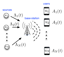
Figure 1: A BS updates $N$ users $u_{1},\cdots,u_{N}$ on information from sources $s_{1},\cdots,s_{N}$, respectively.

We consider a wireless broadcast network consisting of a base-station (BS) and $N$ wireless users $u_{1},\cdots,u_{N}$ in Fig. 1. Each user $u_{i}$ is interested in a type of information generated by a source $s_{i}$, for $i=1,\cdots,N$, respectively. All information is sent in the form of packets by the BS over a noiseless broadcast channel.

We consider a discrete-time system with slot $t=0,1,\cdots$. The packets from the sources (if any) arrive at the BS at the beginning of each slot. The arrivals at the BS for different users are independent of each other, and also independent and identically distributed (i.i.d.) over slots, governed by a Bernoulli distribution. Precisely, by $\Lambda_{i}(t)$ we indicate if a packet from source $s_{i}$ arrives at the BS in slot $t$, where $\Lambda_{i}(t)=1$ if there is a packet, with $P[\Lambda_{i}(t)=1]=p_{i}$; otherwise, $\Lambda_{i}(t)=0$.

We assume that the BS can send at most one packet during each slot, i.e., the BS can update at most one user in each slot. Moreover, we focus on the setting that the BS does not buffer a packet if it is not transmitted in the arriving slot. The no-buffer network is motivated by [2].

By $D(t)\in\{0,1,\cdots N\}$ we denote a decision of the BS in slot $t$, where $D(t)=0$ if no one will be updated in slot $t$ and $D(t)=i$ for $i=1,\cdots,N$ if user $u_{i}$ is scheduled to be updated in slot $t$. A scheduling algorithm $\theta=\{D(0),D(1),\cdots\}$ specifies a decision for each slot. Next, we will define an age of information as our design criterion.

II-B Age of information model

The age of information implies the freshness of the information at the users. We initialize the ages of all arriving packets at the BS to be zero. The age of information at a user becomes one on receiving a packet, due to one slot of the transmission time. Let $X_{i}(t)$ be the age of information for user $u_{i}$ in slot $t$ before the BS makes a scheduling decision. Suppose that the age increases linearly with slots. Then, the dynamics of the age of information for user $u_{i}$ is

$$X_{i}(t+1)=\left\{\begin{array}[]{ll}1&\text{if $\Lambda_{i}(t)=1$ and $D(t)=i$;}\\ X_{i}(t)+1&\text{else,}\end{array}\right.$$

where the age in the next slot is one if the user gets updated on the new information; otherwise, the age increases by one. Since the BS can update at most one user for each slot, $X_{i}(t)\geq 1$ for all $i$, $X_{i}(t)\neq X_{j}(t)$ for all $i\neq j$, and $\sum_{i=1}^{N}X_{i}(t)\geq 1+2+\cdots+N$ for all $t$.

II-C Problem formulation

We define the average age under a scheduling algorithm $\theta$ by

$$\limsup_{T\rightarrow\infty}\frac{1}{T+1}E_{\theta}\left[\sum_{t=0}^{T}\sum_{i=1}^{N}X_{i}(t)\right],$$

where $E_{\theta}$ represents the conditional expectation, given that the algorithm $\theta$ is employed. Note that we focus on the total age, but our work can be easily extended to a weighted sum of the ages. Our goal is to develop a low-complexity scheduling algorithm whose average age is close to the minimum by leveraging the Whittle’s methodology [4].

III Scheduling algorithm design

We will develop a scheduling algorithm based on restless bandits [3] in stochastic control theory. To reach the goal, in this section, we start with casting our problem as a restless multi-armed bandit problem [3], followed by introducing the Whittle index [4] as a solution to the multi-armed bandit problem. A challenge of this approach is to obtain the Whittle index. We then explicitly derive the Whittle index in a simpler way using a post-action age. We finally propose a scheduling algorithm based on the Whittle index.

III-A Restless bandits and Whittle’s approach

A restless bandit generalizes a classic bandit by allowing the bandit to keep evolving under a passive action, but in a distinct way from its continuation under an active action. However, the restless bandits problem, in general, is PSPACE-hard [3]. Whittle hence investigates a relaxed version, where a constraint on the number of active bandits for each slot is replaced by the expected number. With this relaxation, Whittle then applies a Lagrangian approach to decouple the multi-armed bandit problem into multiple sub-problems.

We can regard each user in our problem as a restless bandit. Following the Whittle’s approach, we can decouple our problem into $N$ sub-problems. A sub-problem consists of a user $u_{i}$ and adheres to the network model in Section II with $N$ = 1, except for an additional cost $C$ for updating the user. In each sub-problem, we aim at determining whether or not the user should be updated for each slot, in order to strike a balance between the updating cost and the cost incurred by age. In fact, the cost $C$ is a scalar Lagrange multiplier in the Lagrangian approach. Since each sub-problem consists of a single user, hereafter we omit the index $i$ for simplicity.

III-B Decoupled sub-problem

We formulate the sub-problem as a Markov decision process (MDP), with the components [15] as follows.

States: We define the state $\mathbf{s}(t)$ of the MDP in slot $t$ by $\mathbf{s}(t)=(X(t),\Lambda(t))$. This is an infinite-state MDP as the age is possibly unbounded.

Actions: Let $a(t)\in\{0,1\}$ be an action of the MDP in slot $t$ indicating the BS’s decision, where $a(t)=1$ if the BS decides to update the user and $a(t)=0$ if the BS decides to idle.

Transition probabilities: The transition probability from state $\mathbf{s}=(x,\lambda)$ to state $\mathbf{s}^{\prime}$ under action $a(t)=a$ is:

$$P[\mathbf{s}^{\prime}=(x+1,1)|\mathbf{s}=(x,\lambda),a(t)=0]=p;$$

$$P[\mathbf{s}^{\prime}=(x+1,0)|\mathbf{s}=(x,\lambda),a(t)=0]=1-p;$$

$$P[\mathbf{s}^{\prime}=(1,1)|\mathbf{s}=(x,1),a(t)=1]=p;$$

$$P[\mathbf{s}^{\prime}=(1,0)|\mathbf{s}=(x,1),a(t)=1]=1-p;$$

$$P[\mathbf{s}^{\prime}=(x+1,1)|\mathbf{s}=(x,0),a(t)=1]=p;$$

$$P[\mathbf{s}^{\prime}=(x+1,0)|\mathbf{s}=(x,0),a(t)=1]=1-p.$$

Cost: Let $C(\mathbf{s}(t),a(t))$ be an immediate cost if action $a(t)$ is taken in slot $t$ under state $\mathbf{s}(t)$, with the definition as follows.

$$C\Bigl{(}\textbf{s}(t)=(x,\lambda),a(t)=a\Bigr{)}\triangleq(x+1-x\cdot a\cdot\lambda)+C\cdot a,$$ (1)

where the first part $x+1-x\cdot a\cdot\lambda$ is the resulting age in the next slot and the second part is the incurred cost for updating the user.

A policy $\mu=\{a(0),a(1),\cdots\}$ of the MDP specifies an action for each slot. A policy $\mu$ is history dependent if $a(t)$ depends on $\mathbf{s}(0),\cdots,\mathbf{s}(t)$ and $a(0)\cdots,a(t-1)$. A policy is stationary if $a(t_{1})=a(t_{2})$ when $\mathbf{s}(t_{1})=\mathbf{s}(t_{2})$ for any $t_{1},t_{2}$. Moreover, a randomized policy chooses an action with a probability, while a deterministic policy chooses an action with certainty.

The average cost under a policy $\mu$ is defined by

$$\limsup_{T\rightarrow\infty}\frac{1}{T+1}E_{\mu}\left[\sum_{t=0}^{T}C(\mathbf{s}(t),a(t))\right].$$

Definition 1.

A policy $\mu$ (that can be history dependent) is cost-optimal if it minimizes the average cost.

The objective of the MDP is to find a policy $\mu$ that minimizes the average cost. According to [15], there may not exist a cost-optimal policy that is stationary or deterministic. Hence, in the next section, we aim at investigating a cost-optimal policy.

III-C Characterizing a cost-optimal policy

We will study structures of a cost-optimal policy in this section. First, we show that a cost-optimal policy is stationary and deterministic as follows.

Theorem 2.

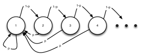
Figure 2: The age $X(t)$ under the policy $f$ forms a DTMC.

There exists a stationary and deterministic policy that is cost-optimal, independent of initial state $\mathbf{s}(0)$.

Proof.

Given initial state $\mathbf{s}(0)=\mathbf{s}$, we define the expected total discounted cost [15] under policy $\mu$ by

$$J_{\alpha}(\mathbf{s};\mu)=\limsup_{T\rightarrow\infty}E_{\mu}\left[\sum_{t=0}^{T}\alpha^{t}C(\mathbf{s}(t),a(t))|\mathbf{s}(0)=\mathbf{s}\right],$$

where $0<\alpha<1$ is a discount factor. Moreover, let $J_{\alpha}(\mathbf{s})=\min_{\mu}J_{\alpha}(\mathbf{s};\mu)$ be the minimum expected total discounted cost. A policy that minimizes the expected total $\alpha$-discounted cost is called $\alpha$-optimal policy.

According to [16], a deterministic stationary policy is cost-optimal if the following two conditions hold.

1. There exists a deterministic stationary policy of the MDP such that the associated average cost is finite: Let $f$ be the deterministic stationary policy of always choosing the action $a(t)=1$ for each slot $t$ if there is an arrival. The age $X(t)$ under the policy $f$ forms a discrete-time Markov chain (DTMC) in Fig. 2. The steady-state distribution $\boldsymbol{\pi}=(\pi_{1},\pi_{2},\cdots,)$ of the DTMC is

   $$\pi_{i}=p(1-p)^{i-1}\,\,\,\,\text{for all $i=1,2,\cdots$}.$$

   Hence, the average age is

   $$\sum_{i=1}^{\infty}i\pi_{i}=\sum_{i=1}^{\infty}ip(1-p)^{i-1}=\frac{1}{p}.$$

   On the other hand, the average updating cost is $C\cdot p$ as the arrival probability is $p$. Hence, the average cost under the policy $f$ is the average age (i.e., $1/p$) plus the average updating cost (i.e., $C\cdot p$), which is finite and yields the result.

2. There exists a non-negative $L$ such that the relative cost function $h_{\alpha}(\mathbf{s})\triangleq J_{\alpha}(\mathbf{s})-J_{\alpha}(\mathbf{0})\geq-L$ for all $\mathbf{s}$ and $\alpha$, where $\mathbf{0}$ is a reference state: Similar to [2], we can show that $J_{\alpha}(x,\lambda)$ is a non-decreasing function in age $x$ given arrival indicator $\lambda$; moreover, $J_{\alpha}(x,\lambda)$ is a non-increasing function in $\lambda$ given $x$. Then, we can choose $L=0$ by choosing the reference state $\mathbf{0}=(0,1)$.

By verifying the two conditions, the theorem immediately follows from [16]. ∎

Next, we further investigate a cost-optimal policy by showing that it is a special type of deterministic stationary policy.

Definition 3.

A threshold-type policy is a deterministic stationary policy of the MDP. The action for state $(x,0)$ is to idle, for all $x$. Moreover, if the action for state $(x,1)$ is to update, then the action for state $(x+1,1)$ is to update as well. In other words, there exists a threshold $\bar{X}\in\{1,2,\cdots\}$ such that the action is to update if there is an arrival and the age is greater than or equal to $\bar{X}$; otherwise, the action is to idle.

Theorem 4.

If $C\geq 0$, then there exists a policy of the threshold type that is cost-optimal.

Proof.

It is obvious that an optimal action for state $(x,0)$ is to idle if $C\geq 0$. To establish the optimality of the threshold structure for state $(x,1)$, we need the discounted cost optimality equation (see the proof of Theorem 2 and [15]): if the first condition in the proof of Theorem 2 holds, then for any state $\mathbf{s}$ the minimum expected total discounted cost $J_{\alpha}(\mathbf{s})$ satisfies

$$J_{\alpha}(\mathbf{s})=\min_{a\in\{0,1\}}C(\mathbf{s},a)+\alpha E[J_{\alpha}(\mathbf{s}^{\prime})],$$

where the expectation is taken over all possible next state $\mathbf{s}^{\prime}$ reachable from state $\mathbf{s}$.

Subsequently, we intend to prove that an $\alpha$-optimal policy is the threshold type. Let $\mathscr{J}_{\alpha}(\mathbf{s};a)=C(\mathbf{s};a)+\alpha E[J_{\alpha}(\mathbf{s}^{\prime})]$. Then, $J_{\alpha}(\mathbf{s})=\min_{a\in\{0,1\}}\mathscr{J}_{\alpha}(\mathbf{s};a)$. Moreover, an $\alpha$-optimal action for state $\mathbf{s}$ is $\operatornamewithlimits{arg\,min}_{a\in\{0,1\}}\mathscr{J}_{\alpha}(\mathbf{s};a)$ [15]. Suppose an $\alpha$-optimal action for state $(x,1)$ is to update, i.e.,

$$\mathscr{J}_{\alpha}(x,1;1)-\mathscr{J}_{\alpha}(x,1;0)\leq 0.$$

Then, an $\alpha$-optimal action for state $(x+1,1)$ is still to update since

$$\mathscr{J}_{\alpha}(x+1,1;1)-\mathscr{J}_{\alpha}(x+1,1;0)$$

$$= \left(1+C+\alpha E[J_{\alpha}(1,\lambda^{\prime})]\right)-\left(x+2+\alpha E[J_{\alpha}(x+2,\lambda^{\prime})]\right)$$

$$\mathop{\leq}^{(a)} \left(1+C+\alpha E[J_{\alpha}(1,\lambda^{\prime})]\right)-\left(x+1+\alpha E[J_{\alpha}(x+1,\lambda^{\prime})]\right)$$

$$= J_{\alpha}(x,1;1)-J_{\alpha}(x,1;0)\leq 0,$$

where (a) results from the non-decreasing function of $J_{\alpha}(x,\lambda)$ in $x$ given $\lambda$ (see proof of Theorem 2). Hence, an $\alpha$-optimal policy is the threshold type.

Finally, we conclude that a cost-optimal policy is the threshold type as well since a cost-optimal policy is the limit point of $\alpha$-optimal policies with $\alpha\rightarrow 1$ if both conditions in the proof of Theorem 2 hold [2] . ∎

To find an optimal threshold for minimizing the average cost, we explicitly derive the average cost in the next theorem.

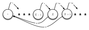
Figure 3: The post-action age $Y(t)$ under the threshold-type policy forms a DTMC.

Theorem 5.

Given the threshold-type policy with the threshold $\bar{X}\in\{1,2,\cdots\}$, then the average cost, denoted by $\mathscr{C}(\bar{X})$, under the policy is

$$\mathscr{C}(\bar{X})=\frac{\frac{\bar{X}^{2}}{2}+(\frac{1}{p}-\frac{1}{2})\bar{X}+\frac{1}{p^{2}}-\frac{1}{p}+C}{\bar{X}+\frac{1-p}{p}}.$$ (2)

Proof.

Let $Y(t)$ be the age after an action in slot $t$; precisely, if $\mathbf{s}(t)=(x,\lambda)$ and $a(t)=a$, then $Y(t)=x+1-x\cdot a\cdot\lambda$. Note that $Y(t)$, called post-action age (similar to the post-decsion state [17]), is different from the pre-action age $X(t)$.

The post-action age $Y(t)$ forms a DTMC in Fig. 3. Moreover, we associate each state in the DTMC with a cost. The DTMC incurs the cost of $C+1$ in slot $t$ when the post-action age in slot $t$ is $Y(t)=1$ since the post-action age $Y(t)=1$ implies that the BS updates the user, while incurring the cost of $y$ in slot $t$ when the post-action age is $Y(t)=y\neq 1$. Then, the steady-state distribution $\boldsymbol{\pi}=(\pi_{1},\pi_{2},\cdots)$ of the DTMC is

$$\pi_{i}=\left\{\begin{array}[]{ll}\frac{1}{\bar{X}+\frac{1-p}{p}}&\text{if $i=1,\cdots,\bar{X}$;}\\ \frac{1}{\bar{X}+\frac{1-p}{p}}(1-p)^{i-\bar{X}}&\text{if $i=\bar{X}+1,\cdots$}.\end{array}\right.$$

Therefore, the average cost of the DTMC is

$$(1+C)\pi_{1}+\sum_{i=2}^{\infty}i\pi_{i}=\frac{\frac{\bar{X}^{2}}{2}+(\frac{1}{p}-\frac{1}{2})\bar{X}+\frac{1}{p^{2}}-\frac{1}{p}+C}{\bar{X}+\frac{1-p}{p}}.$$

∎

We want to elaborate on the post-action age in the proof. There might be alternatives for obtaining the average cost as follows:

• As in many literature, e.g., [3], we can find an optimal action for each state by solving the average cost optimality equation [15]. However, we might not arrive at the average cost optimality equation as this is an infinite-state MDP [16]. Even though the average cost optimality equation is established, it is usually hard to solve the optimality equation directly.

• Given threshold $\bar{X}$, then state $(X(t),\Lambda(t))$ forms a two-dimensional DTMC. It is usually hard to solve the steady-state distribution for a multi-dimensional DTMC.

• Given threshold $\bar{X}$, the pre-action age $X(t)$ forms a DTMC as well. However, we cannot associate each state with a cost, since the cost depends on not only state but also action (see Eq. (1)). On the contrary, the cost for the post-action age $Y(t)$ is determined by state only.

III-D Deriving the Whittle index

Now, we are ready to define the Whittle index.

Definition 6.

We define the Whittle index $I(\mathbf{s})$ by the cost $C$ that makes both actions for state $\mathbf{s}$ equally desirable.

Theorem 7.

The Whittle index of the sub-problem for state $(x,\lambda)$ is

$$I(x,\lambda)=\left\{\begin{array}[]{ll}0&\text{if $\lambda=0$;}\\ \frac{x^{2}}{2}-\frac{x}{2}+\frac{x}{p}&\text{if $\lambda=1$.}\end{array}\right.$$

Proof.

It is obvious that the Whittle index for state $(x,0)$ is $I(x,0)=0$ as both actions result in the same immediate cost and the same age of next slot if $C=0$.

Let $g(x)=\mathscr{C}(x)$ in Eq. (2) for the domain of $\{x\in\mathbb{R}:x\geq 1\}$. Note that $g(x)$ is strictly convex in the domain. Let $x^{*}$ be the minimizer of $g(x)$. Then, an optimal threshold for minimizing the average cost $\mathscr{C}(\bar{X})$ is either $\lfloor x^{*}\rfloor$ or $\lceil x^{*}\rceil$: the optimal threshold is $\bar{X}^{*}=\lfloor x^{*}\rfloor$ if $\mathscr{C}(\lfloor x^{*}\rfloor)\leq\mathscr{C}(\lceil x^{*}\rceil)$ and $\bar{X}^{*}=\lceil x^{*}\rceil$ if $\mathscr{C}(\lceil x^{*}\rceil)\leq\mathscr{C}(\lfloor x^{*}\rfloor)$. If there is a tie, both choices are optimal.

Hence, both actions for state $(x,1)$ are equally desirable if and only if the age $x$ satisfies

$$\mathscr{C}(x)=\mathscr{C}(x+1),$$

i.e., $x=\lfloor x^{*}\rfloor$ and both thresholds of $x$ and $x+1$ are optimal. By solving the above equation, we obtain the cost to make both actions equally desirable, as the Whittle index in the theorem. ∎

According to Theorem 7, both actions might have a tie. If there is a tie, we break the tie in favor of idling. Then, we can explicitly express the optimal threshold in the next theorem.

Theorem 8.

The optimal threshold for minimizing the average cost is $\bar{X}^{*}=x$ if the cost satisfies $I(x-1,1)\leq C<I(x,1)$, for all $x=1,2,\cdots$.

Proof.

Since $I(x)$ is the cost to make both actions for state $(x,1)$ equally desirable and we break a tie in favor of idling, then the optimal threshold is $\bar{X}^{*}=x+1$ if the cost is $C=I(x)$, for all $x$. We claim that the optimal threshold monotonically increases with cost $C$, and then the theorem follows.

To verify the claim, we can focus on an $\alpha$-optimal policy according to the proof of Theorem 4. Suppose that an $\alpha$-optimal action, associated with a cost $C_{1}$, for state $(x,1)$ is to idle, i.e.,

$$x+1+\alpha E[J_{\alpha}(x+1,\lambda^{\prime})]\leq 1+C_{1}+\alpha E[J_{\alpha}(1,\lambda^{\prime})].$$

Then, an $\alpha$-optimal action, associated with a cost $C_{2}\geq C_{1}$, for state $(x,1)$ is to idle as well since

$$x+1+\alpha E[J_{\alpha}(x+1,\lambda^{\prime})]\leq 1+C_{1}+\alpha E[J_{\alpha}(1,\lambda^{\prime})]$$

$$\leq 1+C_{2}+\alpha E[J_{\alpha}(1,\lambda^{\prime})].$$

Then, the monotonicity is established. ∎

Next, according to [4], we have to demonstrate the indexability defined as follows.

Definition 9.

Given cost $C$, let $\mathbf{S}(C)$ be the set of states $\mathbf{s}$ such that the optimal action for the states is to idle. The sub-problem is indexable if the set $\mathbf{S}(C)$ monotonically increases from the empty set to the entire state space, as $C$ increases from $-\infty$ to $\infty$.

Theorem 10.

The sub-problem is indexable.

Proof.

If $C<0$, the optimal action for every state is to update; as such, $\mathbf{S}(0)=\emptyset$. If $C\geq 0$, then $\mathbf{S}(C)$ is composed of the set $\{\mathbf{s}=(x,0):x=1,2,\cdots\}$ and a set of $(x,1)$ for some $x$’s. According to Theorem 8, the optimal threshold monotonically increases as $C$ increases, and hence the set $\mathbf{S}(C)$ monotonically increases to the entire state space. ∎

III-E Scheduling algorithm design

Now, we are ready to propose a scheduling algorithm based on the Whittle index. For each slot $t$, the BS observes age $X_{i}(t)$ and arrival indicator $\Lambda_{i}(t)$ for every user $u_{i}$; then, update a user $u_{i}$ with the highest value of the Whittle index $I(X_{i}(t),\Lambda_{i}(t))$. We can think of the index $I(X_{i}(t),\Lambda_{i}(t))$ as the cost to update user $u_{i}$. The intuition of the scheduling algorithm is that the BS intends to send the most valuable packet. In Fig. 4, we compare the proposed algorithm with the age-optimal scheduling algorithm in [2] for two users over 100,000 slots. It turns out that the simple index algorithm almost achieves the minimum average age.

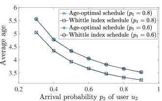
Figure 4: Average age for two users under the proposed Whittle index scheduling algorithm and an age-optimal scheduling algorithm.

IV Conclusion

This paper treated a wireless broadcast network, where many users are interested in different types of information delivered by a base-station. Under a transmission constraint, we studied a transmission scheduling problem, with respect to the age of information. We have proposed a low-complexity scheduling algorithm leveraging the Whittle’s methodology. Numerical studies showed that the proposed algorithm almost minimizes the average age. To investigate a regime under which the proposed algorithm is optimal would be an interesting extension.

References

- [1] S. Kaul, R. D. Yates, and M. Gruteser, “Real-Time Status: How Often Should One Update?” Proc of IEEE INFOCOM, pp. 2731–2735, 2012.
- [2] Y.-P. Hsu, E. Modiano, and L. Duan, “Age of Information: Design and Analysis of Optimal Scheduling Algorithms,” Proc. of IEEE ISIT, pp. 561–565, 2017.
- [3] J. Gittins, K. Glazebrook, and R. Weber, Multi-Armed Bandit Allocation Indices. John Wiley & Sons, 2011.
- [4] P. Whittle, “Restless Bandits: Activity Allocation in a Changing World,” Journal of applied probability, pp. 287–298, 1988.
- [5] R. R. Weber and G. Weiss, “On an index policy for restless bandits,” Journal of Applied Probability, vol. 27, no. 3, pp. 637–648, 1990.
- [6] M. Larranaga, U. Ayesta, and I. M. Verloop, “Stochastic and Fluid Index Policies for Resource Allocation Problems,” Proc. of IEEE INFOCOM, pp. 1230–1238, 2015.
- [7] D. P. Bertsekas, Dynamic Programming and Optimal Control Vol. I and II. Athena Scientific, 2012.
- [8] M. Costa, M. Codreanu, and A. Ephremides, “On the Age of Information in Status Update Systems with Packet Management,” IEEE Trans. Inf. Theory, vol. 62, no. 4, pp. 1897–1910, 2016.
- [9] A. M. Bedewy, Y. Sun, and N. B. Shroff, “Age-Optimal Information Updates in Multihop Networks,” Proc. of IEEE ISIT, pp. 576–580, 2017.
- [10] A. Kosta, N. Pappas, and V. Angelakis, “Age of Information: A New Concept, Metric, and Tool,” Foundations and Trends® in Networking, vol. 12, no. 3, pp. 162–259, 2017.
- [11] Q. He, D. Yuan, and A. Ephremides, “Optimal Link Scheduling for Age Minimization in Wireless Systems,” accepted to IEEE Trans. Inf. Theory, 2017.
- [12] C. Joo and A. Eryilmaz, “Wireless Scheduling for Information Freshness and Synchrony: Drift-based Design and Heavy-Traffic Analysis,” Proc. of IEEE WIOPT, pp. 1–8, 2017.
- [13] I. Kadota, E. Uysal-Biyikoglu, R. Singh, and E. Modiano, “Minimizing Age of Information in Broadcast Wireless Networks,” Proc. of Allerton, 2016.
- [14] R. D. Yates, P. Ciblat, A. Yener, and M. Wigger, “Age-Optimal Constrained Cache Updating,” Proc. of IEEE ISIT, pp. 141–145, 2017.
- [15] M. L. Puterman, Markov Decision Processes: Discrete Stochastic Dynamic Programming. The MIT Press, 1994.
- [16] L. I. Sennott, “Average Cost Optimal Stationary Policies in Infinite State Markov Decision Processes with Unbounded Costs,” Operations Research, vol. 37, pp. 626–633, 1989.
- [17] W. B. Powell, Approximate Dynamic Programming: Solving the Curses of Dimensionality. John Wiley & Sons, 2011.