Blessing of dimensionality: mathematical foundations of the statistical physics of data

Abstract

The concentration of measure phenomena were discovered as the mathematical background of statistical mechanics at the end of the XIX - beginning of the XX century and were then explored in mathematics of the XX-XXI centuries. At the beginning of the XXI century, it became clear that the proper utilisation of these phenomena in machine learning might transform the curse of dimensionality into the blessing of dimensionality.

This paper summarises recently discovered pheno-mena of measure concentration which drastically simplify some machine learning problems in high dimension, and allow us to correct legacy artificial intelligence systems. The classical concentration of measure theorems state that i.i.d. random points are concentrated in a thin layer near a surface (a sphere or equators of a sphere, an average or median level set of energy or another Lipschitz function, etc.).

The new stochastic separation theorems describe the thin structure of these thin layers: the random points are not only concentrated in a thin layer but are all linearly separable from the rest of the set, even for exponentially large random sets. The linear functionals for separation of points can be selected in the form of the linear Fisher’s discriminant.

All artificial intelligence systems make errors. Non-destructive correction requires separation of the situations (samples) with errors from the samples corresponding to correct behaviour by a simple and robust classifier. The stochastic separation theorems provide us by such classifiers and a non-iterative (one-shot) procedure for learning.

1 Introduction: Five “Foundations”, from geometry to probability, quantum mechanics, statistical physics and machine learning

It’s not given us to foretell
How our words will echo through the ages,…

F.I. Tyutchev, English Translation by F.Jude

The Sixth Hilbert Problem was inspired by the “investigations on the foundations of geometry” [1], i.e. by Hilbert’s work “The Foundations of Geometry” [2], which firmly implanted the axiomatic method not only in the field of geometry, but also in other branches of mathematics. The Sixth Problem proclaimed expansion of the axiomatic method beyond existent mathematical disciplines, into physics and further on.

The Sixth Problem sounds very unusual and not purely mathematical. This may be a reason why some great works which have been inspired by this problem have no reference to it. The most famous example is the von Neumann book [3] “Mathematical foundations of quantum mechanics”. John von Neumann was the assistant of Hilbert and they worked together on the mathematical foundation of quantum mechanics. This work was obviously in the framework of the Sixth Problem, but this framework was not mentioned in the book.

In 1933, Kolmogorov answered the Hilbert challenge of axiomatization of the theory of probability [4]. He did not cite the sixth problem but explicitly referred to Hilbert’s “Foundations of Geometry” as the prototype for “the purely mathematical development” of the theory. But Hilbert in his 6th Problem asked for more, for “a rigorous and satisfactory development of the method of the mean values in mathematical physics”. He had in mind statistical physics and “in particular the kinetic theory of gases”. The 6th chapter of Kolmogorov’s book contains a survey of some results of the author and Khinchin about independence and the law of large numbers, and the Appendix includes a description of the 0-1 laws in probability. These are the first steps to a rigorous basis of “the method of mean values”. Ten years later, in 1943, Khinchin published a book “Mathematical foundations of statistical mechanics” [5]. This has brought an answer to the Sixth Problem one step closer, but again without explicit reference to Hilbert’s talk. The analogy between the titles of von Neumann and Khinchin books is obvious.

The main idea of statistical mechanics, in its essence, can be called the blessing of dimensionality: if a system can be presented as a union of many weakly interacting subsystems then, in the thermodynamic limit (when the number of such subsystems tends to infinity), the whole system can be described by relatively simple deterministic relations in the low-dimensional space of macroscopic variables. More means less – in very high-dimensional spaces many differences between sets and functions become negligible (vanish) and the laws become simpler. This point of view on statistical mechanics was developed mainly by Gibbs (1902) (ensemble equivalence) [6] but Khinchin made the following remark about this work: “although the arguments are clear from the logical standpoint, they do not pretend to any analytical rigor”, exactly in the spirit of Hilbert’s request for “a rigorous and satisfactory development”. The devil is in the detail: how should we define the thermodynamic limit and in which sense the ensembles are equivalent? For some rigorously formulated conditions, the physical statements become exact theorems.

Khinchin considered two types of background theorems: ergodic theorems and limit theorems for high-dimensional distributions. He claimed that the foundations of statistical mechanics should be a complete abstraction from the nature of the forces. Limit theorems utilize very general properties of distributions in high dimension, indeed, but the expectations that ergodicity is a typical and universal property of smooth high-dimensional multiparticle Hamiltonian systems were not met [7]. To stress that the ergodicity problem is nontrivial, we have to refer to the Oxtoby–Ulam theorem about metric transitivity of a generic continuous transformation, which preserves volume [8]. (We see that typical properties of continuous transformations differ significantly from typical properties of smooth transformations).

Various programmes proposed for the mathematical foundation of statistical mechanics were discussed, for example, by Dobrushin [9] and Batterman [10]. Despite the impressive proof of ergodicity of some systems (hyperbolic flows or some billiard systems, for example), the Jaynes point of view [11] on the role of ergodicity in the foundations of statistical mechanics now became dominant; the Ergodic Hypothesis is neither necessary nor sufficient condition for the foundation of statistical mechanics (Dobrushin [9] attributed this opinion to Lebowitz, while Jaynes [11] referred to Gibbs [6], who, perhaps, “did not consider ergodicity as relevant to the foundation of the subject”).

Through the efforts of many mathematicians, the limit theorems from probability theory and results about ensemble equivalence from the foundation of statistical physics were developed far enough to become the general theory of measure concentration phenomena. Three works were especially important for our work [12, 13, 14]. The book [15] gives an introduction into the mathematical theory of measure concentration. A simple geometric introduction into this phenomena was given by Ball [16].

Perhaps, the simplest manifestation of measure concentration is the concentration of the volume of the high-dimensional ball near the sphere. Let $V_{n}(r)$ be a volume of the n-dimensional ball of radius $r$. It is useful to stress that the ‘ball’ here is not necessarily Euclidean and means the ball of any norm. Lévy [17] recognised this phenomenon as a very important property of geometry of high-dimensional spaces. He also proved that equidistributions in the balls are asymptotically equivalent in high dimensions to the Gaussian distributions with the same mean value of squared radius. Gibbs de-facto used these properties for sublevel sets of energy to demonstrate equivalence of ensembles (microcanonical distribution on the surface of constant energy and canonical distribution in the phase space with the same mean energy).

Maxwell used the concentration of measure phenomenon in the following settings. Consider a rotationally symmetric probability distribution on the $n$-dimensional unit sphere. Then its orthogonal projection on a line will be a Gaussian distribution with small variance $1/n$ (for large $n$ with high accuracy). This is exactly the Maxwellian distribution for one degree of freedom in a gas (and the distribution on the unit sphere is the microcanonical distribution of kinetic energy of gas, when the potential energy is negligibly small). Geometrically it means that if we look at the one-dimensional projections of the unit sphere then the “observable diameter” will be small, of the order of $1/\sqrt{n}$.

Lévy noticed that instead of orthogonal projections on a straight line we can use any $\eta$-Lipschitz function $f$ (with $\|f(x)-f(y)\|\leq\eta\|x-y\|$). Let points $x$ be distributed on a unit $n$-dimensional sphere with rotationally symmetric probability distribution. Then the values of $f$ will be distributed ‘not more widely’ than a normal distribution around the mean value $\mathbf{E}_{f}$; for all $\varepsilon>0$

$$\mathbf{P}(|f-\mathbf{E}_{f}|\geq\varepsilon)\leq 2\exp\left(-\frac{n\varepsilon^{2}}{2c\eta^{2}}\right),$$

where $c$ is a constant, $c\leq 9\pi^{3}$. Interestingly, if we use in this inequality the median value of $f$, $M_{f}$, instead of the mean, then the estimate of the constant $c$ can be decreased: $c\leq 1$. From the statistical mechanics point of view, this Lévy Lemma describes the upper limit of fluctuations in gas for an arbitrary observable quantity $f$. The only condition is the sufficient regularity of $f$ (Lipschitz property).

Hilbert’s 6th Problem influenced this stream of research either directly (Kolmogorov and, perhaps, Khinchin among others) or indirectly, through the directly affected works. And it keeps to transcend this influence to other areas, including high-dimensional data analysis, data mining, and machine learning.

On the turn of the millennium, Donoho gave a lecture about main problems of high-dimensional data analysis [18] with the impressive subtitle: “The curses and blessings of dimensionality”. He used the term curse of dimensionality “to refer to the apparent intractability of systematically searching through a high-dimensional space, the apparent intractability of accurately approximating a general high-dimensional function, the apparent intractability of integrating a high-dimensional function.” To describe the blessing of dimensionality he referred to the concentration of measure phenomenon, “which suggest that statements about very high-dimensional settings may be made where moderate dimensions would be too complicated.” Anderson et al characterised some manifestations of this phenomenon as “The More, the Merrier” [19].

In 1997, Kainen described the phenomenon of blessing of dimensionality, illustrated them with a number of different examples in which high dimension actually facilitated computation, and suggested connections with geometric phenomena in high-dimensional spaces [20].

The claim of Donoho’s talk was similar to Hilbert’s talk and he cited this talk explicitly. (“My personal research experiences, cited above, convince me of Hilbert’s position, as a long run proposition, operating on the scale of centuries rather than decades.”) The role of Hilbert’s 6th Problem in the analysis of the curse and blessing of dimensionality was not mentioned again.

The blessing of dimensionality and the curse of dimensionality are two sides of the same coin. For example, the typical property of a random finite set in a high-dimensional space is: the squared distance of these points to a selected point are, with high probability close to the average (or median) squared distance. This property drastically simplifies the expected geometry of data (blessing) [21, 22] but, at the same time, makes the similarity search in high dimensions difficult and even useless (curse) [23].

Extension of the 6th Hilbert Problem to data mining and machine learning is a challenging task. There exist no unified general definition of machine learning. Most classical texts consider machine learning through formalisation and analysis of a set of standardised tasks [24, 25, 26]. Traditionally, these tasks are:

• Classification – learning to predict a categorical attribute using values of given attributes on the basis of given examples (supervised learning);

• Regression – learning to predict numerical attributes using values of given attributes on the basis of given examples (supervised learning);

• Clustering – joining of similar objects in several clusters (unsupervised learning) [27];

• Various data approximation and reduction problems: linear and nonlinear principal components [28], principal graphs [29], independent components [30], etc. (clustering can be also considered as a data approximation problem [31]);

• Probability distribution estimation.

For example, Cucker and Smale [24] considered the least square regression problem. This is the problem of the best approximation of an unknown function $f:X\to Y$ from a random sample of pairs $(x,y)\in X\times Y$. Selection of “the best” regression function means minimization of the mean square error deviation of the observed $y$ from the value $f(x)$. They use the concentration inequalities to evaluate the probability that the approximation has a given accuracy.

It is important to mention that the Cucker–Smale approach was inspired in particular by J. von Neumann: “We try to write in the spirit of H. Weyl and J. von Neumann’s contributions to the foundations of quantum mechanics” [24]. The J. von Neumann book [3] was a step in the realisation of Hilbert’s 6th problem programme, as we perfectly know. Therefore, the Cucker–Smale “Mathematical foundation of learning” is a grandchild of the 6th problem. This is the fourth “Foundation” (after Kolmogorov, von Neumann, and Khinchin). Indeed, it was an attempt to give a rigorous development of what they “have found to be the central ideas of learning theory”. This problem statement follows Hilbert’s request for “rigorous and satisfactory development of the method of mean values”, but this time the development was done for machine learning instead of mathematical physics.

Cucker and Smale followed Gauss and proved that the least squares solution enjoys remarkable statistical properties. i.e. it provides the minimum variance estimate [24]. Nevertheless, non-quadratic functionals are employed for solution of many problems: to enhance robustness, to avoid oversensitivity to outliers, to find sparse regression with exclusion of non-necessary input variables, etc. [25, 26]. Even non-convex quasinorms and their tropical approximations are used efficiently to provide sparse and robust learning results [32]. Vapnik [26] defined a formalised fragment of machine learning using minimisation of a risk functional that is the mathematical expectation of a general loss function.

M. Gromov [33] proposed a radically different concept of ergosystems which function by building their “internal structure” out of the “raw structures” in the incoming flows of signals. The essential mechanism of egrgosystem learning is goal free and independent of any reinforcement. In a broad sense, loosely speaking, in this concept “structure” = “interesting structure” and learning of structure is goal-free and should be considered as a structurally interesting process.

There are many other approaches and algorithms in machine learning, which use some specific ideas from statistical mechanics: annealing, spin glasses, etc. (see, for example, [34]) and randomization. It was demonstrated recently that the assignment of random parameters should be data-dependent to provide the efficient and universal approximation property of the randomized learner model [35]. Various methods for evaluation of the output weights of the hidden nodes after random generation of new nodes were also tested [35]. Swarm optimization methods for learning with random re-generation of the swarm (“virtual particles”) after several epochs of learning were developed in 1990 [36]. Sequential Monte Carlo methods for learning neural networks were elaborated and tested [37]. A comprehensive overview of the classical algorithms and modern achievements in stochastic approaches to neural networks was performed by Scardapane and Wang [38].

In our paper, we do not discuss these ideas, instead we focus on a deep and general similarity between high-dimensional problems in learning and statistical physics. We summarise some phenomena of measure concentration which drastically affect machine learning problems in high dimension.

2 Waist concentration and random bases in machine learning

After classical works of Fisher [39] and Rosenblatt [40], linear classifiers have been considered as inception of Data Analytics and Machine Learning (see e.g. [26, 41, 42], and references therein). The mathematical machinery powering these developments is based on the concept of linear separability.

Definition 2.1.

Let $\mathcal{X}$ and $\mathcal{Y}$ be subsets of $\mathbb{R}^{n}$. Recall that a linear functional $l$ on $\mathbb{R}^{n}$ separates $\mathcal{X}$ and $\mathcal{Y}$ if there exists a $t\in\mathbb{R}$ such that

$$l(\boldsymbol{x})>t>l(\boldsymbol{y})\ \forall\ \boldsymbol{x}\in\mathcal{X},\ \boldsymbol{y}\in\mathcal{Y}.$$

A set $\mathcal{S}\subset\mathbb{R}^{n}$ is linearly separable if for each $\boldsymbol{x}\in\mathcal{S}$ there exists a linear functional $l$ such that $l(\boldsymbol{x})>l(\boldsymbol{y})$ for all $y\in\mathcal{S}$, $\boldsymbol{y}\neq\boldsymbol{x}$.

If $\mathcal{X}\subset\mathbb{R}^{n}$ is a set of measurements or data samples that are labelled as “Class 1”, and $\mathcal{Y}$ is a set of data labelled as “Class 2” then a functional $l$ separating $\mathcal{X}$ and $\mathcal{Y}$ is the corresponding linear classifier. The fundamental question, however, is whether such functionals exist for the given $\mathcal{X}$ and $\mathcal{Y}$, and if the answer is “Yes” then how to find them?

It is well-known that if (i) $\mathcal{X}$ and $\mathcal{Y}$ are disjoint, (ii) the cardinality, $|\mathcal{X}\cup\mathcal{Y}|$, of $\mathcal{X}\cup\mathcal{Y}$ does not exceed $n+1$, and (iii) elements of $\mathcal{X}\cup\mathcal{Y}$ are in general position, then they are vertices of a simplex. Hence, in this setting, there always is a linear functional $l$ separating $\mathcal{X}$ and $\mathcal{Y}$.

Rosenblatt’s $\alpha$-perceptron [40] used a population of linear threshold elements with random synaptic weights ($A$-elements) as layer before an $R$-element, that is a linear threshold element which learns iteratively (authors of some papers and books called the $R$-elements “perceptrons” and lose the complex structure of $\alpha$-perceptron with a layer of random $A$-elements). The randomly initiated elements of the first layer can undergo selection of the most relevant elements.

According to Rosenblatt [40], any set of data vectors becomes linear separable after transformation by the layer of $A$-elements, if the number of these randomly chosen elements is sufficiently large. Therefore the perceptron can solve any classification problem, where classes are defined by pointing out examples (ostensive definition). But this “sufficiently large” number of random elements depends on the problem and may be large, indeed. It can grow for a classification task proportionally to the number of the examples. The perceptron with sufficiently large number of $A$-elements can approximate binary-valued functions on finite domains with arbitrary accuracy. Recently, the bounds on errors of these approximations are derived [43]. It is proven that unless the number of network units grows faster than any polynomial of the logarithm of the size of the domain, a good approximation cannot be achieved for almost any uniformly randomly chosen function. The results are obtained by application of concentration inequalities.

The method of random projections became popular in machine learning after the Johnson-Lindenstrauss Lemma [44], which states that relatively large sets of $m$ vectors in a high-dimensional Euclidean space $\mathbb{R}^{d}$ can be linearly mapped into a space of much lower dimension $n$ with approximate preservation of distances. This mapping can be constructed (with high probability) as a projection on $n$ random basis vectors with rescaling of the projection with a factor $\sqrt{d}$ [45]. Repeating the projection $O(m)$ times and selecting the best of them, one can achieve the appropriate accuracy of the distance preservation. The number of points $m$ can be exponentially large with $n$ ($m\leq\exp(cn)$).

Two unit random vectors in high dimension are almost orthogonal with high probability. This is a simple manifestation of the so-called waist concentration [13]. A high-dimensional sphere is concentrated near its equator. This is obvious: just project a sphere onto a hyperplane and use the concentration argument for a ball on the hyperplane (with a simple trigonometric factor). This seems highly non-trivial, if we ask: near which equator? The answer is: near each equator. This answer is obvious because of rotational symmetry but it seems to be counter-intuitive.

We call vectors $\boldsymbol{x}$, $\boldsymbol{y}$ from Euclidean space $\mathbb{R}^{n}$ $\varepsilon$-orthogonal if $|(\boldsymbol{x},\boldsymbol{y})|<\varepsilon$ ($\varepsilon>0$). Let $\boldsymbol{x}$ and $\boldsymbol{y}$ be i.i.d. random vectors distributed uniformly (rotationally invariant) on the unit sphere in Euclidean space $\mathbb{R}^{n}$. Then the distribution of their inner product satisfies the inequality (see, for example [16] or [46] and compare to Maxwellian and Lévy’s lemma):

$$\mathbf{P}(|(\boldsymbol{x},\boldsymbol{y})|<\varepsilon)\geq 1-2\exp\left(-\frac{1}{2}n\varepsilon^{2}\right).$$

Proposition 2.1.

Let $\boldsymbol{x}_{1},\ldots,\boldsymbol{x}_{N}$ be be i.i.d. random vectors distributed uniformly (rotationally invariant) on the unit sphere in Euclidean space $\mathbb{R}^{n}$. For

$$\boxed{N<e^{\frac{\varepsilon^{2}n}{4}}\left[\ln\left(\frac{1}{1-\vartheta}\right)\right]^{\frac{1}{2}}}$$ (1)

all vectors $\boldsymbol{x}_{1},\ldots,\boldsymbol{x}_{N}$ are pairwise $\varepsilon$-orthogonal with probability $P>1-\vartheta$. [46]

There are two consequences of this statement: (i) in high dimension there exist exponentially many pairwise almost orthogonal vectors in $\mathbb{R}^{n}$, and (ii) $N$ random vectors are $\varepsilon$-orthogonal with high probability $P>1-\vartheta$ even for exponentially large $N$ (1). Existence of exponentially large $\varepsilon$-orthogonal systems in high-dimensional spaces was discovered in 1993 by Kainen and Kůrková [47]. They introduced the notion of quasiorthogonal dimension, which was immediately utilised in the problem of random indexing of high-dimensional data [21]. The fact that an exponentially large random set consists of pairwise $\varepsilon$-orthogonal vectors with high probability was demonstrated in the work [46] and used for analysis of data approximation problem in random bases. We show that not only such $\varepsilon$-orthogonal sets exist, but also that they are typical in some sense.

$N$ randomly generated vectors $\boldsymbol{x}_{i}$ will be almost orthogonal to a given data vector $\boldsymbol{y}$ (the angle between $\boldsymbol{x}$ and $\boldsymbol{y}$ will be close to $\pi/2$ with probability close to one). Therefore, the coefficients in the approximation of $\boldsymbol{y}$ by a linear combination of $\boldsymbol{x}_{i}$ could be arbitrarily large and the approximation problem will be ill-conditioned, with high probability. The following alternative is proven for approximation by random bases:

• Approximation of a high-dimensional data vector by linear combinations of randomly and independently chosen vectors requires (with high probability) generation of exponentially large “bases”, if we would like to use bounded coefficients in linear combinations.

• If arbitrarily large coefficients are allowed, then the number of randomly generated elements that are sufficient for approximation is even less than dimension. We have to pay for such a reduction of the number of elements by ill-conditioning of the approximation problem.

We have to choose between a well-conditioned approximation problem in exponentially large random bases and an ill-conditional problem in relatively small (moderate) random bases. This dichotomy is fundamental, and it is a direct consequence of the waist concentration phenomenon. In what follows, we will formally present another concentration phenomenon, stochastic separation theorems [48, 49], and outline their immediate applications in AI and neuroscience.

3 Stochastic separation theorems and their applications in Artificial Intelligence systems

3.1 Stochastic separation theorems

Existence of a linear functional that separates two finite sets $\mathcal{X},\mathcal{Y}\subset\mathbb{R}^{n}$ is no longer obvious when $|\mathcal{X}\cup\mathcal{Y}|\gg n$. A possible way to answer both questions could be to cast the problem as a constrained optimization problem within the framework of e.g. support vector machines [26]. The issue with this approach is that theoretical worst-case estimates of computational complexity for determining such functions are of the order $O(|\mathcal{X}\cup\mathcal{Y}|^{3})$ (for quadratic loss functions); a posteriori analysis of experiments on practical use cases, however, suggest that the complexity could be much smaller and than $O(|\mathcal{X}\cup\mathcal{Y}|^{3})$ and reduce to linear or even sublinear in $|\mathcal{X}\cup\mathcal{Y}|$ [50].

This apparent discrepancy between the worst-case estimates and a-posteriori evaluation of computational complexities can be resolved if concentration effects are taken into account. If the dimension $n$ of the underlying topological vector space is large then random finite but exponentially large in $n$ samples are linearly separable, with high probability, for a range of practically relevant classes of distributions. Moreover, we show that the corresponding separating functionals can be derived using Fisher linear discriminants [39]. Computational complexity of the latter is linear in $|\mathcal{X}\cup\mathcal{Y}|$. It can be made sub-linear too in if proper sampling is used to estimate corresponding covariance matrices. As we have shown in [49], the results hold for i.i.d. random points from equidistributions in a ball, a cube, and from distributions that are products of measures with bounded support. The conclusions are based on stochastic separation theorems for which the statements for relevant classes of distributions are provided below.

Theorem 3.1 (Equidistribution in $\mathbb{B}_{n}(1)$ [48, 49]).

Let $\{\boldsymbol{x}_{1},\ldots,\boldsymbol{x}_{M}\}$ be a set of $M$ i.i.d. random points from the equidustribution in the unit ball $\mathbb{B}_{n}(1)$. Let $0<r<1$, and $\rho=\sqrt{1-r^{2}}$. Then

$$\mathbf{P}\left(\|\boldsymbol{x}_{M}\|>r\mbox{ and }\left(\boldsymbol{x}_{i},\frac{\boldsymbol{x}_{M}}{\|\boldsymbol{x}_{M}\|}\right)<r\mbox{ for all }i\neq M\right)\geq 1-r^{n}-0.5(M-1)\rho^{n};$$ (2)

$$\mathbf{P}\left(\|\boldsymbol{x}_{j}\|>r\mbox{ and }\left(\boldsymbol{x}_{i},\frac{\boldsymbol{x}_{j}}{\|\boldsymbol{x}_{j}\|}\right)<r\mbox{ for all }i,j,\,i\neq j\right)\geq 1-Mr^{n}-0.5M(M-1)\rho^{n};$$ (3)

$$\mathbf{P}\left(\|\boldsymbol{x}_{j}\|>r\mbox{ and }\left(\frac{\boldsymbol{x}_{i}}{\|\boldsymbol{x}_{i}\|},\frac{\boldsymbol{x}_{j}}{\|\boldsymbol{x}_{j}\|}\right)<r\mbox{ for all }i,j,\,i\neq j\right)\geq 1-Mr^{n}-M(M-1)\rho^{n}.$$ (4)

The proof of the theorem can be illustrated with Fig. 1. The probability that a single element, $\boldsymbol{x}_{M}$, belongs to the difference $\mathbb{B}_{n}(1)\setminus\mathbb{B}_{n}(r)$ of two $n$-balls centred at $O$ is not smaller than $1-r^{n}$. Consider the hyperplane

$$l(\boldsymbol{x})=r,\mbox{ where }l(\boldsymbol{x})=\left(\boldsymbol{x},\frac{\boldsymbol{x}_{M}}{\|\boldsymbol{x}_{M}\|}\right).$$

This hyperplane partitions the unit ball $\mathbb{B}_{n}(1)$ centred at $O$ into two disjoint subsets: the spherical cap (shown as grey shaded area in Fig. 1) and the rest of the ball. The element $\boldsymbol{x}_{M}$ is in the shaded area and is on the line containing the vector $OO^{\prime}$. The volume of this spherical cap does not exceed the volume of the half-ball of radius $\rho$ centred at $O^{\prime}$ (the ball $\mathbb{B}_{n}(\rho)$ is shown as a blue dashed circle in the figure). Recall that

$$\mathbf{P}(A_{1}\&A_{2}\&\ldots\&A_{m})\geq 1-\sum_{i}(1-\mathbf{P}(A_{i}))\mbox{ for any events }A_{1},\ldots,A_{m}.$$ (5)

This assures that (2) holds. Applying the same argument to all elements of the set $\mathcal{S}$ results in (3). Finally, to show that (4) holds, observe that the length of the segment $OA$ on the tangent line to the sphere $\mathbb{S}_{n-1}(\rho)$ centred at $O^{\prime}$ is always smaller than $r=|OO^{\prime}|$. Hence the cosine of the angle between an element from $(\mathbb{B}_{n}(1)\setminus\mathbb{B}_{n}(r))\setminus\mathbb{B}_{n}(\rho)$ and the vector $OO^{\prime}$ is bounded from above by $\cos(\angle(OA^{\prime},OO^{\prime}))=r$. The estimate now follows from (5).

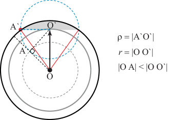
Figure 1: Illustration to Theorem 3.1.

According to Theorem 3.1, the probability that a single element $\boldsymbol{x}_{M}$ from the sample $\mathcal{S}=\{\boldsymbol{x}_{1},\dots,\boldsymbol{x}_{M}\}$ is linearly separated from the set $\mathcal{S}\setminus\{\boldsymbol{x}_{M}\}$ by the hyperplane $l(x)=r$ is at least

$$1-r^{n}-0.5(M-1)\left(1-r^{2}\right)^{\frac{n}{2}}.$$

This probability estimate depends on both $M=|\mathcal{S}|$ and dimensionality $n$. An interesting consequence of the theorem is that if one picks a probability value, say $1-\vartheta$, then the maximal possible values of $M$ for which the set $\mathcal{S}$ remains linearly separable with probability that is no less than $1-\vartheta$ grows at least exponentially with $n$. In particular, the following holds

Corollary 3.1.

Let $\{\boldsymbol{x}_{1},\ldots,\boldsymbol{x}_{M}\}$ be a set of $M$ i.i.d. random points from the equidustribution in the unit ball $\mathbb{B}_{n}(1)$. Let $0<r,\vartheta<1$, and $\rho=\sqrt{1-r^{2}}$. If

$$M<2({\vartheta-r^{n}})/{\rho^{n}},$$ (6)

then $\mathbf{P}((\boldsymbol{x}_{i},\boldsymbol{x}_{M}{)}<r\|\boldsymbol{x}_{M}\|\mbox{ for all }i=1,\ldots,M-1)>1-\vartheta.$ If

$$M<({r}/{\rho})^{n}\left(-1+\sqrt{1+{2\vartheta\rho^{n}}/{r^{2n}}}\right),$$ (7)

then $\mathbf{P}((\boldsymbol{x}_{i},\boldsymbol{x}_{j})<r\|\boldsymbol{x}_{i}\|\mbox{ for all }i,j=1,\ldots,M,\,i\neq j)\geq 1-\vartheta.$

In particular, if inequality (7) holds then the set $\{\boldsymbol{x}_{1},\ldots,\boldsymbol{x}_{M}\}$ is linearly separable with probability $p>1-\vartheta$.

The linear separability property of finite but exponentially large samples of random i.i.d. elements is not restricted to equidistributions in $\mathbb{B}_{n}(1)$. As has been noted in [22], it holds for equidistributions in ellipsoids as well as for the Gaussian distributions. Moreover, it can be generalized to product distributions in a unit cube. Consider, e.g. the case when coordinates of the vectors $\boldsymbol{x}=(X_{1},\dots,X_{n})$ in the set $\mathcal{S}$ are independent random variables $X_{i}$, $i=1,\dots,n$ with expectations $\overline{X}_{i}$ and variances $\sigma_{i}^{2}>\sigma_{0}^{2}>0$. Let $0\leq X_{i}\leq 1$ for all $i=1,\dots,n$. The following analogue of Theorem 3.1 can now be stated.

Theorem 3.2 (Product distribution in a cube [49]).

Let $\{\boldsymbol{x}_{1},\ldots,\boldsymbol{x}_{M}\}$ be i.i.d. random points from the product distribution in a unit cube. Let

$$R_{0}^{2}=\sum_{i}\sigma_{i}^{2}\geq n\sigma_{0}^{2},$$

and $0<\delta<2/3$. Then

$$\begin{split}&\mathbf{P}\left(1-\delta\leq\frac{\|\boldsymbol{x}_{j}-\overline{\boldsymbol{x}}\|^{2}}{R^{2}_{0}}\leq 1+\delta\mbox{ and }\left(\frac{\boldsymbol{x}_{i}-\overline{\boldsymbol{x}}}{R_{0}},\frac{\boldsymbol{x}_{M}-\overline{\boldsymbol{x}}}{\|\boldsymbol{x}_{M}-\overline{\boldsymbol{x}}\|}\right)<\sqrt{1-\delta}\mbox{ for all }i,j,\,i\neq M\right)\\ &\geq 1-2M\exp\left(-2\delta^{2}R_{0}^{4}/n\right)-(M-1)\exp\left(-2R_{0}^{4}(2-3\delta)^{2}/n\right);\end{split}$$ (8)

$$\begin{split}&\mathbf{P}\left(1-\delta\leq\frac{\|\boldsymbol{x}_{j}-\overline{\boldsymbol{x}}\|^{2}}{R^{2}_{0}}\leq 1+\delta\mbox{ and }\left(\frac{\boldsymbol{x}_{i}-\overline{\boldsymbol{x}}}{R_{0}},\frac{\boldsymbol{x}_{j}-\overline{\boldsymbol{x}}}{\|\boldsymbol{x}_{j}-\overline{\boldsymbol{x}}\|}\right)<\sqrt{1-\delta}\mbox{ for all }i,j,\,i\neq j\right)\\ &\geq 1-2M\exp\left(-2\delta^{2}R_{0}^{4}/n\right)-M(M-1)\exp\left(-2R_{0}^{4}(2-3\delta)^{2}/n\right).\end{split}$$ (9)

The proof is based on concentration inequalities in product spaces [14, 51]. Numerous generalisations of Theorems 3.1, 3.2 are possible for different classes of distributions, for example, for weakly dependent variables, etc.

Linear separability, as an inherent property of data sets in high dimension, is not necessarily confined to cases whereby a linear functional separates a single element of a set from the rest. Theorems 3.1, 3.2 be generalized to account for $m$-tuples, $m>1$ too. An example of such generalization is provided in the next theorem.

Theorem 3.3 (Separation of $m$-tuples [52]).

Let $\mathcal{X}=\{\boldsymbol{x}_{1},\dots,\boldsymbol{x}_{M}\}$ and $\mathcal{Y}=\{\boldsymbol{x}_{M+1},\dots,\boldsymbol{x}_{M+k}\}$ be i.i.d. samples from the equidistribution in $\mathbb{B}_{n}(1)$. Let $\mathcal{Y}_{c}=\{\boldsymbol{x}_{M+r_{1}},\dots,\boldsymbol{x}_{M+r_{m}}\}$ be a subset of $m$ elements from $\mathcal{Y}$ such that

$$\beta_{2}(m-1)\leq\sum_{r_{j},\ r_{j}\neq r_{i}}\left(\boldsymbol{x}_{M+r_{i}},\boldsymbol{x}_{M+r_{j}}\right)\leq\beta_{1}(m-1)\ \mbox{for all}\ i=1,\dots,m.$$ (10)

Then

$$\mathbf{P}\left(\exists\mbox{ a linear functional separating }\mathcal{X}\mbox{ and }\mathcal{Y}_{c}\right)\geq\max_{\varepsilon\in(0,1)}(1-(1-\varepsilon)^{n})^{m}\left(1-\frac{\Delta(\varepsilon,m)^{\frac{n}{2}}}{2}\right)^{M},$$ (11)

where

$$\Delta(\varepsilon,m)=1-\frac{1}{m}\left(\frac{(1-\varepsilon)^{2}+\beta_{2}(m-1)}{\sqrt{1+(m-1)\beta_{1}}}\right)^{2},$$

subject to:

$$(1-\varepsilon)^{2}+\beta_{2}(m-1)>0,\ 1+(m-1)\beta_{1}>0.$$

The separating linear functional is again the inner product, and the separating hyperplane can be taken in the form [52]:

$$l(\boldsymbol{x})=r;\;\mbox{ where }l(\boldsymbol{x})=\left(\boldsymbol{x},\frac{\bar{\boldsymbol{y}}}{\|\bar{\boldsymbol{y}}\|}\right),\;r=\frac{1}{\sqrt{m}}\left(\frac{(1-\varepsilon)^{2}+\beta_{2}(m-1)}{\sqrt{1+(m-1)\beta_{1}}}\right),$$ (12)

and $\varepsilon$ is the maximizer of the nonlinear program in the right-hand side of (11), and $\bar{\boldsymbol{y}}=\frac{1}{m}\sum_{i=1}^{m}\boldsymbol{x}_{M+r_{i}}$. To see this, observe that $\|\boldsymbol{x}_{M+r_{i}}\|\geq 1-\varepsilon$, $\varepsilon\in(0,1)$, for all $i=1,\dots,m$, with probability $(1-(1-\varepsilon)^{n})^{m}$. With this probability the following estimate holds:

$$\left(\frac{\bar{\boldsymbol{y}}}{\|\bar{\boldsymbol{y}}\|},\boldsymbol{x}_{M+r_{i}}\right)\geq\frac{1}{m\|\bar{\boldsymbol{y}}\|}\left((1-\varepsilon)^{2}+\beta_{2}(m-1)\right).$$

Hence

$$\frac{1}{m}\left(1+(m-1)\beta_{1}\right)\geq\left(\bar{\boldsymbol{y}},\bar{\boldsymbol{y}}\right)\geq\frac{1}{m}\left((1-\varepsilon)^{2}+\beta_{2}(m-1)\right),$$

and $l(\boldsymbol{x})$ in (12) is the required functional (see also Fig. 1).

If the elements of $\mathcal{Y}_{c}$ are uncorrelated, i.e. the values of $\beta_{1}(m-1),\beta_{2}(m-1)$ are small, then the distance from the spherical cap induced by linear functional (12) to the center of the ball decreases as $O(1/\sqrt{m})$. This means that the lower-bound probability estimate in (11) is expected to decrease too. On the other hand, if the elements of $\mathcal{Y}_{c}$ are all positively correlated, i.e. $1\geq\beta_{1}>\beta_{2}>0$, then one can derive a lower-bound probability estimate which does not depend on $m$.

Peculiar properties of data in high dimension, expressed in terms of linear separability, have several consequences and applications in the realm of Artificial Intelligence and Machine Learning of which the examples are provided in the next sections.

3.2 Correction of legacy AI systems

Legacy AI systems, i.e. AI systems that have been deployed and are currently in operation, are becoming more and more wide-spread. Well-known commercial examples are provided by global multi-nationals, including Google, IMB, Amazon, Microsoft, and Apple. Numerous open-source legacy AIs have been created to date, together with dedicated software for their creation (e.g. Caffe [53], MXNet [54], Deeplearning4j [55], and Tensorflow [56] packages). These AI systems require significant computational and human resources to build. Regardless of resources spent, virtually any AI and/or machine learning-based systems are likely to make a mistake. Real-time correction of these mistakes by re-training is not always viable due to the resources involved. AI re-training is not necessarily desirable either, since AI’s performance after re-training may not always be guaranteed to exceed that of the old one. We can, therefore, formulate the technical requirements for the correction procedures. Corrector should: (i) be simple; (ii) not change the skills of the legacy system; (iii) allow fast non-iterative learning; and (iv) allow correction of new mistakes without destroying of previous corrections.

A possible remedy to this issue is the AI correction method [22] based on stochastic separation theorems. Suppose that at a time instance $t$ values of signals from inputs, outputs, and internal state of a legacy AI system could be combined together to form a single measurement object, $\boldsymbol{x}=(x_{1},\dots,x_{n})$. All $n$ entries in this object are numerical values, and each measurement $\boldsymbol{x}$ corresponds to a relevant decision of the AI system at time $t$. Over the course of the system’s existence a set $\mathcal{S}$ of such measurements is collected. For each element in the set $\mathcal{S}$ a label “correct” or “incorrect” is assigned, depending on external evaluation of the system’s performance. Elements corresponding to “incorrect” labels are then filtered out and dealt with separated by an additional subsystem, a corrector. A diagram illustrating the process is shown in Fig. 2.

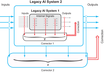
Figure 2: Cascade of AI correctors

In this diagram, the original legacy AI system (shown as Legacy AI System 1) is supplied with a corrector altering its responses. The combined new AI system can in turn be augmented by another corrector, leading to a cascade of AI correctors (see Fig. 2).

If distributions modelling elements of the set $\mathcal{S}$ are e.g. an equidistribution in a ball or an ellipsoid, product of measures distribution, a Gaussian etc., then

• Theorems 3.1–3.3 guarantee that construction of such AI correctors can be achieved using mere linear functionals.

• These linear functions admit a closed-form formulae (Fisher linear discriminant) and can be determined in a non-iterative way.

• Availability of explicit closed-form formulae in the form of Fisher discriminant offers major computational benefits as it eliminates the need to employ iterative and more computationally expensive alternatives such as e.g. SVMs.

• If a cascade of correctors is employed, performance of the corrected system drastically improves [22].

The results, perhaps, can be generalized to other classes of distributions that are regular enough to enjoy the stochastic separability property.

The corrector principle has been demonstrated in [22] for a legacy AI system in the form of a convolutional neural network trained to detect pedestrians in images. AI errors were set to be false positives, and the corrector system had to remove labeled false positives by a single linear functional. Detailed description of the experiment is provided in [22], and a performance snapshot is shown in Fig. 3.

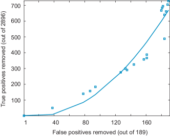
Figure 3: True positives removed as a function of false positives removed by a single-functional corrector [22].

Dimensionality $n$ of the vectors $\boldsymbol{x}$ was $2000$. As we can see from Fig. 3, single linear functionals are capable of removing several errors of a legacy AI without compromising the system’s performance. Note that AI errors, i.e. false positives, were chosen at random and have not been grouped or clustered to take advantage of positive correlation. (The definition of clusters could vary [27].) As the number of errors to be removed grows, performance starts to deteriorate. This is in agreement with our theoretical predictions (Theorem 3.3).

3.3 Knowledge transfer between AI systems

Legacy AI correctors can be generalized to a computational framework for automated AI knowledge transfer whereby labelling of the set $\mathcal{S}$ is provided by an external AI system. AI knowledge transfer has been in the focus of growing attention during last decade [57]. Application of stochastic separation theorems to AI knowledge transfer was proposd in [52], and the corresponding functional diagram of this automated setup is shown in Fig. 4.

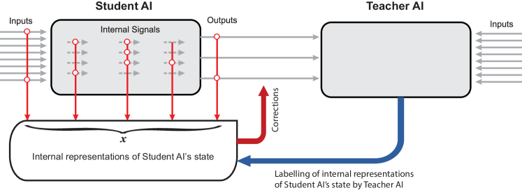
Figure 4: AI Knowledge Transfer

In this setup a student AI, denoted as $\mathrm{AI}_{s}$, is monitored by a teacher AI, denoted as $\mathrm{AI}_{t}$. Over a period of activity system $\mathrm{AI}_{s}$ generates a set $\mathcal{S}$ of objects $\boldsymbol{x}$, $\boldsymbol{x}\in\mathbb{R}^{n}$. Exact composition of the set $\mathcal{S}$ depends on a task at hand. If $\mathrm{AI}_{s}$ outputs differ to that of $\mathrm{AI}_{t}$ for the same input then an error is registered in the system. Objects $\boldsymbol{x}\in\mathcal{S}$ associated with errors are combined into the set $\mathcal{Y}$. The process gives rise to two disjoint sets:

$$\mathcal{X}=\{\boldsymbol{x}_{1},\dots,\boldsymbol{x}_{M}\},\ \mathcal{X}=\mathcal{S}\setminus\mathcal{Y},\mbox{ and }\mathcal{Y}=\{\boldsymbol{x}_{M+1},\dots,\boldsymbol{x}_{M+k}\}.$$

Having created these two sets, knowledge transfer from $\mathrm{AI}_{t}$ to $\mathrm{AI}_{s}$ can now be organized in accordance with Algorithm 1. Note that data regularization and whitening are included in the pre-processing step of Algorithm 1.

Algorithm 1 AI Knowledge Transfer/Correction [52]

1. Pre-processing

   1. Centering. For the given set $\mathcal{S}$, determine the set average, $\bar{\boldsymbol{x}}(\mathcal{S})$, and generate sets $\mathcal{S}_{c}$

      $$\begin{array}[]{ll}{\mathcal{S}_{c}}&=\{\boldsymbol{x}\in\mathbb{R}^{n}\ |\boldsymbol{x}=\boldsymbol{\xi}-\bar{\boldsymbol{x}}(\mathcal{S}),\ \boldsymbol{\xi}\in\mathcal{S}\},\\ {\mathcal{Y}_{c}}&=\{\boldsymbol{x}\in\mathbb{R}^{n}\ |\boldsymbol{x}=\boldsymbol{\xi}-\bar{\boldsymbol{x}}(\mathcal{S}),\ \boldsymbol{\xi}\in\mathcal{Y}\}.\end{array}$$

   2. Regularization. Determine covariance matrices $\mathrm{Cov}(\mathcal{S}_{c})$, $\mathrm{Cov}(\mathcal{S}_{c}\setminus\mathcal{Y}_{c})$ of the sets $\mathcal{S}_{c}$ and $\mathcal{S}_{c}\setminus\mathcal{Y}_{c}$. Let $\lambda_{i}(\mathrm{Cov}(\mathcal{S}_{c}))$, $\lambda_{i}(\mathrm{Cov}(\mathcal{S}_{c}\setminus\mathcal{Y}_{c}))$ be their corresponding eigenvalues, and $h_{1},\dots,h_{n}$ be the eigenvectors of $\mathrm{Cov}(\mathcal{S}_{c})$. If some of $\lambda_{i}(\mathrm{Cov}(\mathcal{S}_{c}))$, $\lambda_{i}(\mathrm{Cov}(\mathcal{S}_{c}\setminus\mathcal{Y}_{c}))$ are zero or if the ratio $\frac{\max_{i}\{\lambda_{i}(\Sigma(\mathcal{S}_{c}))\}}{\min_{i}\{\lambda_{i}(\Sigma(S_{c}))\}}$ is too large, project $\mathcal{S}_{c}$ and $\mathcal{Y}_{c}$ onto appropriately chosen set of $m<n$ eigenvectors, $h_{n-m+1},\dots,h_{n}$:

      $$\begin{array}[]{ll}{\mathcal{S}_{r}}&=\{\boldsymbol{x}\in\mathbb{R}^{n}\ |\boldsymbol{x}=H^{T}\boldsymbol{\xi},\ \boldsymbol{\xi}\in\mathcal{S}_{c}\},\\ {\mathcal{Y}_{r}}&=\{\boldsymbol{x}\in\mathbb{R}^{n}\ |\boldsymbol{x}=H^{T}\boldsymbol{\xi},\ \boldsymbol{\xi}\in\mathcal{Y}_{c}\},\end{array}$$

      where $H=\left(h_{n-m+1}\cdots h_{n}\right)$ is the matrix comprising of $m$ significant principal components of $\mathcal{S}_{c}$.

   3. Whitening. For the centred and regularized dataset $\mathcal{S}_{r}$, derive its covariance matrix, $\mathrm{Cov}(\mathcal{S}_{r})$, and generate whitened sets

      $$\begin{array}[]{ll}{\mathcal{S}_{w}}&=\{\boldsymbol{x}\in\mathbb{R}^{m}\ |\boldsymbol{x}=\mathrm{Cov}(\mathcal{S}_{r})^{-\frac{1}{2}}\boldsymbol{\xi},\ \boldsymbol{\xi}\in\mathcal{S}_{r}\},\\ {\mathcal{Y}_{w}}&=\{\boldsymbol{x}\in\mathbb{R}^{m}\ |\boldsymbol{x}=\mathrm{Cov}(\mathcal{S}_{r})^{-\frac{1}{2}}\boldsymbol{\xi},\ \boldsymbol{\xi}\in\mathcal{Y}_{r}\}.\end{array}$$

2. Knowledge transfer

   1. Clustering. Pick $p\geq 1$, $p\leq k$, $p\in\mathbb{N}$, and partition the set $\mathcal{Y}_{w}$ into $p$ clusters $\mathcal{Y}_{w,1},\dots\mathcal{Y}_{w,p}$ so that elements of these clusters are, on average, pairwise positively correlated. That is there are $\beta_{1}\geq\beta_{2}>0$ such that:

      $$\beta_{2}(|\mathcal{Y}_{w,i}|-1)\leq\sum_{\xi\in\mathcal{Y}_{w,i}\setminus\{\boldsymbol{x}\}}\left(\boldsymbol{\xi},\boldsymbol{x}\right)\leq\beta_{1}(|\mathcal{Y}_{w,i}|-1)\ \mbox{for any}\ \boldsymbol{x}\in\mathcal{Y}_{w,i}.$$

   2. Construction of Auxiliary Knowledge Units. For each cluster $\mathcal{Y}_{w,i}$, $i=1,\dots,p$, construct separating linear functionals $\ell_{i}$ and thresholds $c_{i}$:

      $$\begin{array}[]{ll}\ell_{i}(\boldsymbol{x})&=\left(\frac{\boldsymbol{w}_{i}}{\|\boldsymbol{w}_{i}\|},\boldsymbol{x}\right),\\ \boldsymbol{w}_{i}&=\left(\mathrm{Cov}(\mathcal{S}_{w}\setminus\mathcal{Y}_{w,i})+\mathrm{Cov}(\mathcal{Y}_{w,i})\right)^{-1}\left(\bar{\boldsymbol{x}}(\mathcal{Y}_{w,i})-\bar{\boldsymbol{x}}(\mathcal{S}_{w}\setminus\mathcal{Y}_{w,i})\right),\\ c_{i}&=\min_{\boldsymbol{\xi}\in\mathcal{Y}_{w,i}}\left(\frac{\boldsymbol{w}_{i}}{\|\boldsymbol{w}_{i}\|},\boldsymbol{\xi}\right),\end{array}$$

      where $\bar{\boldsymbol{x}}(\mathcal{Y}_{w,i})$, $\bar{\boldsymbol{x}}(\mathcal{S}_{w}\setminus\mathcal{Y}_{w,i})$ are the averages of $\mathcal{Y}_{w,i}$ and $\mathcal{S}_{w}\setminus\mathcal{Y}_{w,i}$, respectively. The separating hyperplane is $\ell_{i}(\boldsymbol{x})=c_{i}$.

   3. Integration. Integrate Auxiliary Knowledge Units into decision-making pathways of $\mathrm{AI}_{s}$. If, for an $\boldsymbol{x}$ generated by an input to $\mathrm{AI}_{s}$, any of $\ell_{i}(\boldsymbol{x})\geq c_{i}$ then report $\boldsymbol{x}$ accordingly (swap labels, report as an error etc.)

The algorithm can be used for AI correctors too. Similar to AI correction, AI knowledge transfer can be cascaded as well. Specific examples and illustrations of AI knowledge transfer based on stochastic separation theorems are discussed in [52].

3.4 Grandmother cells, memory, and high-dimensional brain

Stochastic separation theorems are a generic phenomenon, and their applications are not limited to AI and machine learning systems. An interesting consequence of these theorems for neuroscience has been discovered and presented in [58]. Recently, it has been shown that in humans new memories can be learnt very rapidly by supposedly individual neurons from a limited number of experiences [59]. Moreover, neurons can exhibit remarkable selectivity to complex stimuli, the evidence that has led to debates around the existence of the so-called “grandmother” and “concept” cells [60, 61, 62], and their role as elements of a declarative memory. These findings suggest that not only the brain can learn rapidly but also it can respond selectively to “rare” individual stimuli. Moreover, experimental evidence indicates that such a cognitive functionality can be delivered by single neurons [59, 60, 61]. The fundamental questions, hence, are: How is this possible? and What could be the underlying functional mechanisms?

It has been shown in [58] that stochastic separation theorems offer a simple answer to these fundamental questions. In particular, extreme neuronal selectivity and rapid learning can already be explained by these theorems. Model-wise, explanation of extreme selectivity is based on conventional and widely accepted phenomenological generic description of neural response to stimulation. Rapid acquisition of selective response to multiple stimuli by single neurons is ensured by classical Hebbian synaptic plasticity [63].

4 Conclusion

Twenty-three Hilbert’s problems created important “focus points” for the concentration of efforts of mathematicians for a century. The Sixth Problem differs significantly from the other twenty-two problems. It is very far from being a purely mathematical problem. It seems to be impossible to imagine it’s “final solution”. The Sixth Problem is a “programmatic call” [64], and it works:

• We definitely know that the Sixth Problem had great influence on the formulation of the mathematical foundation of quantum mechanics [3] and on the development of axiomatic quantum field theory [65].

• We have no doubt (but the authors have no direct evidence) that Sixth Problem has significantly affected research in the foundation of probability theory [4] and statistical mechanics [5].

• The modern theory of measure concentration phenomena has direct relations to the mathematical foundations of probability and statistical mechanics, uses results of Kolmogorov and Khinchin (among others), and definitely helps to create “a rigorous and satisfactory development of the method of the mean values…”.

• Some of the recent attempts of rigorous approach to machine learning [24] used parts of the Sixth Problem programme [3] as a prototype for their conceptual approach.

• The modern idea of blessing of dimensionality in high-dimensional data analysis [18, 19, 48] is, in its essence, an extension and further development of ideas from the mathematical foundations of statistical mechanics.

The classical measure concentration theorems state that random points in a highly-dimensional data distribution are concentrated in a thin layer near an average or median level set of a Lipschitz function. The stochastic separation theorems describe the fine structure of these thin layers: the random points are all linearly separable from the rest of the set even for exponentially large random sets. Of course, for all these concentration and separation theorems the probability distribution should be “genuinely” high-dimensional. Equidistributions in balls or ellipsoids or the products of distributions with compact support and non-vanishing variance are the simple examples of such distributions. Various generalizations are possible.

For which dimensions does the blessing of dimensionality work? This is a crucial question. The naïve point of view that dimension of data is just a number of coordinates is wrong. This is the dimension of the dataspace, where data are originally situated. The notion of intrinsic dimension of data is needed [66, 67]. The situation when the number of data points $N$ is less (or even much less) than the dimension $d$ of the data space is not exotic. Moreover, Donoho [18] considered the property $d>N$ as a generic case in the “post-classical world” of data analysis. In such a situation we really explore data on a $d-1$ dimensional plane and should modestly reduce our high-dimensional claim. Projection of data on that plane can be performed by various methods. We can use as new coordinates projections of points on the known datapoints or Pearson’s correlation coefficients, when it is suitable, for example, when the datapoints are fragments of time series or large spectral images, etc. In these new coordinates the datatable becomes a square matrix and further dimensionality reduction could be performed using good old PCA (principal component analysis), or its nonlinear versions like principal manifolds [28] or neural autoencoders [68].

A standard example can be found in [69]: the initial dataspace consisted of fluorescence diagrams and had dimension $5.2\cdot 10^{5}$. There were 62 datapoints, and a combination of correlation coordinates with PCA showed intrinsic dimension 4 or 5. For selection of relevant principal components the Kaiser rule, the broken stick models or other heuristical or statistical methods can be used [70].

Similar preprocessing ritual is helpful even in more “classical” cases when $d<N$. The correlation (or projection) transformation is not essential here, but formation of relevant features with dimension reduction is important. If after model reduction and whitening (transformation of coordinates to get the unit covariance matrix, step i.c in Algorithm 1) the new dimension $D\gtrsim 100$ then for $\lesssim 10^{6}$ datapoints we can expect that the stochastic separation theorems work with probability $>99\%$. Thus separation of errors with Fisher’s linear discriminant is possible, and many other “blessing of dimensionality benefits” are achievable. Of course, some additional hypotheses about the distribution functions are needed for a rigorous proof, but there is practically no chance to check them a priori and the validation of the whole system a posteriori is necessary. In smaller dimensions (for example, less than 10), nonlinear data approximation methods can work well capturing the intrinsic complexity of data, like principal graphs do [29, 71].

We have an alternative: either essentially high-dimensional data with thin shell concentrations, stochastic separation theorems, and efficient linear methods, or essentially low-dimensional data with efficient complex nonlinear methods. There is a problem of the ‘no man’s land’ in-between. To explore this land, we can extract the most interesting low-dimensional structure and then consider the residual as an essentially high-dimensional random set, which obeys stochastic separation theorems. We do not know now a theoretically justified efficient approach to this area, but here we should say following Hilbert: “Wir müssen wissen, wir werden wissen” (“We must know, we shall know”).

The authors declare that they have no competing interests.

Both authors made substantial contributions to conception, proof of the theorems, analysis of applications, drafting the article, revising it critically, and final approval of the version to be published.

This work was supported by Innovate UK grants KTP009890 and KTP010522. IT was supported by the Russian Ministry of Education and Science, projects 8.2080.2017/4.6 (assessment and computational support for knowledge transfer algorithms between AI systems) and 2.6553.2017/BCH Basic Part.

References

- [1] Hilbert D. 1902 Mathematical problems. Bull. Amer. Math. Soc. 8(10), 437–479. (doi:10.1090/S0002-9904-1902-00923-3)
- [2] Hilbert D. 1902 The Foundations of Geometry. La Salle IL: Open court publishing Company. See http://www.gutenberg.org/ebooks/17384.
- [3] Von Neumann J. 1955 Mathematical Foundations of Quantum Mechanics. Princeton: Princeton University Press. (English translation from German Edition, Springer, Berlin, 1932.)
- [4] Kolmogorov AN. 1956 Foundations of the Theory of Probability. New York: Chelsea Publ. (English translation from German edition, Springer, Berlin, 1933.)
- [5] Khinchin AY. 1949 Mathematical Foundations of Statistical Mechanics. New York: Courier Corporation. (English translation from the Russian edition, Moscow – Leningrad, 1943.)
- [6] Gibbs GW. 1960 [1902] Elementary Principles in Statistical Mechanics, Developed With Especial Reference to the Rational Foundation of Thermodynamics. Dover Publications, New York.
- [7] Markus L, Meyer KR. 1974 Generic Hamiltonian Dynamical Systems are Neither Integrable Nor Ergodic. Memoirs of Amer. Math. Soc. 144. (http://dx.doi.org/10.1090/memo/0144)
- [8] Oxtoby JC, Ulam SM. 1941 Measure-preserving homeomorphisms and metrical transitivity. Ann. Math. 42. 874–920. (doi:10.2307/1968772)
- [9] Dobrushin RL. 1997 A mathematical approach to foundations of statistical mechanics. Atti dei Convegni Lincei – Accademia Nazionale dei Lincei 131, 227–244. See http://www.mat.univie.ac.at/esiprpr/esi179.pdf
- [10] Batterman RW. 1998 Why equilibrium statistical mechanics works: universality and the renormalization group. Philos. Sci. 65, 183–208. (doi:10.1086/392634)
- [11] Jaynes ET. 1967 Foundations of probability theory and statistical mechanics. In Delaware Seminar in the Foundations of Physics. Springer, Berlin – Heidelberg, 77–101. (doi:10.1007/978-3-642-86102-4_6
- [12] Giannopoulos AA, Milman VD. 2000 Concentration property on probability spaces. Adv. Math. 156. 77–106. (doi:10.1006/aima.2000.1949)
- [13] Gromov M. 2003 Isoperimetry of waists and concentration of maps. Geom. Funct. Anal. 13, 178–215. (doi:10.1007/s00039-009-0703-1)
- [14] Talagrand M. 1995 Concentration of measure and isoperimetric inequalities in product spaces. Publications Mathematiques de l’IHES 81, 73–205. (doi:10.1007/BF02699376)
- [15] Ledoux M. 2001 The Concentration of Measure Phenomenon. (Mathematical Surveys & Monographs No. 89). Providence: AMS. (doi:10.1090/surv/089)
- [16] Ball K. 1997 An Elementary Introduction to Modern Convex Geometry. Flavors of Geometry, Vol. 31. Cambridge, UK: MSRI Publications. See http://citeseerx.ist.psu.edu/viewdoc/summary?doi=10.1.1.43.4601.
- [17] Lévy P. 1951 Problèmes concrets d’analyse fonctionnelle. Paris: Gauthier-Villars.
- [18] Donoho DL. 2000 High-dimensional data analysis: The curses and blessings of dimensionality. AMS Math Challenges Lecture, 1, 32 pp. See http://statweb.stanford.edu/donoho/Lectures/AMS2000/Curses.pdf.
- [19] Anderson J, Belkin M, Goyal N, Rademacher L, Voss J. 2014 The More, the Merrier: the Blessing of dimensionality for learning large Gaussian mixtures, Journal of Machine Learning Research: Workshop and Conference Proceedings 35, 1–30. See http://proceedings.mlr.press/v35/anderson14.pdf.
- [20] Kainen PC.1997 Utilizing geometric anomalies of high dimension: when complexity makes computation easier. In Computer-Intensive Methods in Control and Signal Processing: The Curse of Dimensionality. New York, Springer, 283–294. (10.1007/978-1-4612-1996-5_18)
- [21] Hecht-Nielsen R. 1994 Context vectors: General-purpose approximate meaning representations self-organized from raw data. In Zurada J, Marks R, Robinson C, eds. Computational Intelligence: Imitating Life. New York: IEEE Press, 43–56.
- [22] Gorban AN, Romanenko I, Burton R, Tyukin I. 2016 One-trial correction of legacy AI systems and stochastic separation theorems. See arXiv:1610.00494 [stat.ML]
- [23] Pestov V. 2013 Is the -NN classifier in high dimensions affected by the curse of dimensionality? Comput. Math. Appl. 65, 1427–1437. (doi:10.1016/j.camwa.2012.09.011)
- [24] Cucker F, Smale S. 2002 On the mathematical foundations of learning. Bull. Amer. Math. Soc., 39, 1–49. (doi:10.1090/S0273-0979-01-00923-5)
- [25] Friedman J, Hastie T, Tibshirani R. 2009 The Elements of Statistical Learning. New York: Springer. (doi:10.1007/978-0-387-84858-7)
- [26] Vapnik V. 2000 The Nature of Statistical Learning Theory. New York: Springer. (doi:10.1007/978-1-4757-3264-1)
- [27] Xu R, Wunsch D. 2008. Clustering. Hoboken: John Wiley & Sons. (doi:10.1002/9780470382776)
- [28] Gorban AN, Kégl B, Wunsch D, Zinovyev A. (Eds.) 2008 Principal Manifolds for Data Visualisation and Dimension Reduction. Lect. Notes Comput. Sci. Eng., Vol. 58. Berlin – Heidelberg: Springer. (doi:10.1007/978-3-540-73750-6)
- [29] Gorban AN, Zinovyev A. 2010 Principal manifolds and graphs in practice: from molecular biology to dynamical systems. Int. J. Neural Syst. 20, 219–232. (doi:10.1142/S0129065710002383)
- [30] Hyvärinen A, Oja E. 2000 Independent component analysis: algorithms and applications. Neural Netw. 13, 41–430. (doi:10.1016/S0893-6080(00)00026-5)
- [31] Mirkin B. 2012 Clustering: A Data Recovery Approach. Boca Raton: CRC Press. (doi:10.1201/b13101)
- [32] Gorban AN, Mirkes EM, Zinovyev A. 2016. Piece-wise quadratic approximations of arbitrary error functions for fast and robust machine learning. Neural Netw. 84 (2016), 28–38. (doi:10.1016/j.neunet.2016.08.007)
- [33] Gromov M. 2011 Structures, Learning and Ergosystems: Chapters 1-4, 6. IHES, Bures-sur-Ivette, Île-de-France. See http://www.ihes.fr/gromov/PDF/ergobrain.pdf.
- [34] Engel A, Van den Broeck C. 2001 Statistical Mechanics of Learning. Cambridge, UK: Cambridge University Press.
- [35] Wang D, Li M. 2017 Stochastic configuration networks: Fundamentals and algorithms.IEEE Trans. On Cybernetics 47, 3466–3479. (doi:10.1109/TCYB.2017.2734043)
- [36] Gorban AN. 1990 Training Neural Networks, Moscow: USSR-USA JV “ParaGraph”. (doi:10.13140/RG.2.1.1784.4724)
- [37] De Freitas N, Andrieu C, Højen-Sørensen P, Niranjan M, Gee A. 2001 Sequential Monte Carlo methods for neural networks. In Sequential Monte Carlo Methods in Practice. New York: Springer, 359–379. (doi:10.1007/978-1-4757-3437-9_17)
- [38] Scardapane S, Wang D. 2017 Randomness in neural networks: an overview. WIREs Data Mining Knowl. Discov. 7, e1200. (doi:doi.org/10.1002/widm.1200)
- [39] Fisher RA. 1936 The use of multiple measurements in taxonomic problems. Ann. Hum. Genet. 7, 179–188. (doi:10.1111/j.1469-1809.1936.tb02137.x)
- [40] Rosenblatt F. 1962 Principles of Neurodynamics: Perceptrons and the Theory of Brain Mechanisms. Washington DC: Spartan Books. See http://www.dtic.mil/docs/citations/AD0256582.
- [41] Duda RD, Hart PE, and Stork DG. 2012 Pattern classification. New York: John Wiley and Sons.
- [42] Aggarwal CC. 2015 Data Mining: The Textbook. Cham – Heidelberg – New York – Dordrecht – London: Springer. (doi:10.1007/978-3-319-14142-8)
- [43] Kůrková V, Sanguineti M. 2017 Probabilistic lower bounds for approximation by shallow perceptron networks. Neural Netw. 91, 34–41. (doi:10.1016/j.neunet.2017.04.003)
- [44] Johnson WB, Lindenstrauss J. 1984 Extensions of Lipschitz mappings into a Hilbert space. Contemp. Math. 26, 189–206. (doi:10.1090/conm/026/737400)
- [45] Dasgupta S, Gupta A. 2003 An elementary proof of a theorem of Johnson and Lindenstrauss. Random Structures & Algorithms 22, 60–65. (doi:10.1002/rsa.10073)
- [46] Gorban AN, Tyukin I, Prokhorov D, Sofeikov K. 2016 Approximation with random bases: Pro et contra. Inf. Sci. 364–365, 129–145. (doi:10.1016/j.ins.2015.09.021)
- [47] Kainen P, Kůrková V. 1993 Quasiorthogonal dimension of Euclidian spaces. Appl. Math. Lett. 6, 7–10. (doi:10.1016/0893-9659(93)90023-G)
- [48] Gorban AN, Tyukin IY, Romanenko I. 2016. The blessing of dimensionality: Separation theorems in the thermodynamic limit. IFAC-PapersOnLine 49, 64–69. See doi:10.1016/j.ifacol.2016.10.755).
- [49] Gorban AN, Tyukin IY. 2017 Stochastic separation theorems. Neural Netw. 94, 255–259. (doi:10.1016/j.neunet.2017.07.014)
- [50] Chapelle O. 2007 Training a Support Vector Machine in the Primal. Neural Comput. 19, 1155–1178. doi:10.1162/neco.2007.19.5.1155)
- [51] Hoeffding W. 1963. Probability inequalities for sums of bounded random variables. J. Amer. Statist. Assoc. 301, 13–30. (doi:10.1080/01621459.1963.10500830)
- [52] Tyukin IY, Gorban AN, Sofeikov K, Romanenko I. 2017 Knowledge transfer between artificial intelligence systems. See arXiv:1709.01547 [cs.AI].
- [53] Jia Y. 2013 Caffe: An open source convolutional architecture for fast feature embedding. See http://caffe.berkeleyvision.org/.
- [54] Chen T, Li M, Li Y, Lin M, Wang N, Xiao T, Xu B, Zhang C, Zhang Z. 2015 MXNet: A Flexible and Efficient Machine Learning Library for Heterogeneous Distributed Systems. See https://github.com/dmlc/mxnet.
- [55] Team DD. 2016 Deeplearning4j: Open-source distributed deep learning for the JVM, Apache Software Foundation License 2.0. See http://deeplearning4j.org.
- [56] Abadi M, Agarwal A, Barham P et al. 2015 TensorFlow: Large-scale machine learning on heterogeneous systems. Software available from An open-source software library for Machine Intelligence. See https://www.tensorflow.org/.
- [57] Buchtala O, Sick B. 2007 Basic technologies for knowledge transfer in intelligent systems. In Artificial Life, ALIFE’07. New York: IEEE Press. 251–258. (10.1109/ALIFE.2007.367804)
- [58] Tyukin IY, Gorban AN, Calvo C, Makarova J, Makarov VA. 2017 High-dimensional brain. A tool for encoding and rapid learning of memories by single neurons. See arXiv:1710.11227 [q-bio.NC].
- [59] Ison MJ, Quian Quiroga R, Fried I. 2015 Rapid encoding of new memories by individual neurons in the human brain. Neuron 87:220–230. (doi:10.1016/j.neuron.2015.06.016)
- [60] Quian Quiroga R, Reddy, L, Kreiman, G, Koch, C, Fried, I. 2005 Invariant visual representation by single neurons in the human brain. Nature 435, 1102–1107. (doi:10.1038/nature03687)
- [61] Viskontas IV, Quian Quiroga R, Fried, I. 2009. Human medial temporal lobe neurons respond preferentially to personally relevant images. Proc. Nat. Acad. Sci. 106, 21329–21334. (doi:10.1073/pnas.0902319106)
- [62] Quian Quiroga, R. 2012 Concept cells: the building blocks of declarative memory functions. Nat. Rev. Neurosci. 13, 587–597. (doi:10.1038/nrn3251)
- [63] Oja E. 1982 A simplified neuron model as a principal component analyzer. J. Math. Biol. 15, 267–273. (doi:10.1007/BF00275687)
- [64] Corry L. 1997 David Hilbert and the axiomatization of physics (1894–1905). Arch. Hist. Exact Sci. 51, 83–198. (doi:10.1007/BF00375141)
- [65] Wightman AS. 1976 Hilbert’s sixth problem: Mathematical treatment of the axioms of physics. In Browder FE (ed.). Mathematical Developments Arising from Hilbert Problems. Proceedings of Symposia in Pure Mathematics. XXVIII. AMS, 147–240. (doi:10.1090/pspum/028.1/0436800)
- [66] Kégl B. 2003 Intrinsic dimension estimation using packing numbers. In Advances in neural information processing systems 15 (NIPS 2002), Cambridge, US: MIT Press, 697–704.
- [67] Levina E, Bickel PJ. 2005 Maximum likelihood estimation of intrinsic dimension. In Advances in neural information processing systems 17 (NIPS 2004). Cambridge, US: MIT Press, 777–784.
- [68] Bengio Y. 2009 Learning deep architectures for AI. Found. Trends Mach. Learn. 2, 1–127. (doi:10.1561/2200000006)
- [69] Moczko E, Mirkes EM, Ceceres C, Gorban AN, Piletsky S. 2016 Fluorescence-based assay as a new screening tool for toxic chemicals. Sci. Rep. 6, 33922. (doi:10.1038/srep33922)
- [70] Cangelosi R, Goriely A. 2007 Component retention in principal component analysis with application to cDNA microarray data. Biol. Direct 2, 2. (doi:10.1186/1745-6150-2-2)
- [71] Zinovyev A, Mirkes E. 2013. Data complexity measured by principal graphs. Comput. Math. Appl. 65, 1471–1482. (doi:10.1016/j.camwa.2012.12.009)