Isovector and flavor-diagonal charges of the nucleon

Abstract

We present an update on the status of the calculations of isovector and flavor-diagonal charges of the nucleon. The calculations of the isovector charges are being done using ten $2+1+1$-flavor HISQ ensembles generated by the MILC collaboration covering the range of lattice spacings $a\approx$ 0.12, 0.09, 0.06 $\mathop{\rm fm}\nolimits$ and pion masses $M_{\pi}\approx$ 310, 220, 130 $\mathop{\rm MeV}\nolimits$. Excited-states contamination is controlled by using four-state fits to two-point correlators and three-states fits to the three-point correlators. The calculations of the disconnected diagrams needed to estimate flavor-diagonal charges are being done on a subset of six ensembles using the stocastic method. Final results are obtained using a simultaneous fit in $M_{\pi}^{2}$, the lattice spacing $a$ and the finite volume parameter $M_{\pi}L$ keeping only the leading order corrections.

1 Introduction

This talk presents an update on results given in Refs. Bhattacharya:2015wna ; Bhattacharya:2015esa ; Bhattacharya:2016zcn on isovector and flavor diagonal charges of the nucleon using our clover-on-HISQ lattice approach. A summary of the $2+1+1$-flavor HISQ ensembles generated by the MILC collaboration Bazavov:2012xda , and the number of measurements made on them in the ongoing clover-on-HISQ study is given in Table 1. The improvements made since the results reported in Refs. Bhattacharya:2015wna ; Bhattacharya:2015esa ; Bhattacharya:2016zcn are

• cost-effective increase in statistics using the truncated solver method and the coherent source sequential propagator technique.

• The correction for possible bias in the truncated solver method is now made on all ensembles.

• Addition of a second physical mass ensemble at weaker coupling, $a06m135$.

• Excited-state contamination (ESC) is controlled using 4-states in the analysis of the 2-point correlation functions and 3-states for the 3-point functions.

• Fits to 2- and 3-point functions are done using the full covariance matrix in the mimimization of $\chi^{2}$.

• A simultaneous fit in $a$, $M_{\pi}$ and $M_{\pi}L$ is used to extract physical results in the limits $a\to 0$, $M_{\pi}=135$ MeV and $M_{\pi}L\to\infty$ from lattice data obtained at different values of $a$, $M_{\pi}$ and $M_{\pi}L$.

Associated results for the isovector form factors, $G_{A}(Q^{2})$, $\tilde{G}_{P}(Q^{2})$, $G_{E}(q^{2})$ and $G_{M}(q^{2})$, on these ensembles were presented by Yong-Chull Jang at this conference Jang:2017 .

Ensemble ID	$a$ (fm)	$M_{\pi}^{\rm sea}$ (MeV)	$M_{\pi}^{\rm val}$ (MeV)	$L^{3}\times T$	$M_{\pi}^{\rm val}L$	$N_{\text{conf}}$	$N_{\rm meas}^{\rm HP}$	$N_{\rm meas}^{\rm AMA}$
$a12m310$	0.1207(11)	305.3(4)	310(3)	$24^{3}\times 64$	4.55	1013	8104	64,832
$a12m220S$	0.1202(12)	218.1(4)	225(2)	$24^{3}\times 64$	3.29	946	3784	60,544
$a12m220$	0.1184(10)	216.9(2)	228(2)	$32^{3}\times 64$	4.38	744	2976	47,616
$a12m220L$	0.1189(9)	217.0(2)	228(2)	$40^{3}\times 64$	5.49	1010	8080	68,680
$a09m310$	0.0888(8)	312.7(6)	313(3)	$32^{3}\times 96$	4.51	2264	9056	114,896
$a09m220$	0.0872(7)	220.3(2)	226(2)	$48^{3}\times 96$	4.79	964	3856	123,392
$a09m130$	0.0871(6)	128.2(1)	138(1)	$64^{3}\times 96$	3.90	883	7064	84,768
$a06m310$	0.0582(4)	319.3(5)	320(2)	$48^{3}\times 144$	4.52	1000	8000	64,000
$a06m310^{\ast}$						500	2000	64,000
$a06m220$	0.0578(4)	229.2(4)	235(2)	$64^{3}\times 144$	4.41	650	2600	41,600
$a06m220^{\ast}$						650	2600	41,600
$a06m135$	0.0568(1)	135.5(2)	136(2)	$96^{3}\times 192$	3.74	322	1288	20,608

Table 1: Summary of the 2+1+1-flavor HISQ ensembles generated by the MILC Collaboration Bazavov:2012xda and used in our clover-on-HISQ study. The $a06m310^{\ast}$ and the $a06m220^{\ast}$ ensembles represent a second analysis with larger source smearings, $\sigma=12$ and $11$, respectively, as described in Ref. Bhattacharya:2016zcn .

2 Controlling excited-state contamination

Our goal is to extract the matrix elements of various bilinear quark operators between ground state nucleons. The lattice operator $\chi(x)=\epsilon^{abc}\left[{q_{1}^{a}}^{T}(x)C\gamma_{5}\frac{(1\pm\gamma_{4})}{2}q_{2}^{b}(x)\right]q_{1}^{c}(x)$ used to create and annihilate the nucleon state couples to the nucleon, all its excitations and multiparticle states with the same quantum numbers. The correlation functions, therefore, get contributions from all these intermediate states. This ESC can be evaluated and controlled using fits including as many states as the data allow in the spectral decomposition of the two- and three-point functions. In our study we use:

$$C^{\text{2pt}}(t_{f},t_{i})={|{\cal A}_{0}|}^{2}e^{-aM_{0}(t_{f}-t_{i})}+{|{\cal A}_{1}|}^{2}e^{-aM_{1}(t_{f}-t_{i})}+{|{\cal A}_{2}|}^{2}e^{-aM_{2}(t_{f}-t_{i})}+{|{\cal A}_{3}|}^{2}e^{-aM_{3}(t_{f}-t_{i})}+\ldots\,,$$ (1)

$$C^{\text{3pt}}_{\Gamma}(t_{f},t,t_{i}) =|{\cal A}_{0}|^{2}\langle 0|\mathcal{O}_{\Gamma}|0\rangle e^{-aM_{0}(t_{f}-t_{i})}+{}|{\cal A}_{1}|^{2}\langle 1|\mathcal{O}_{\Gamma}|1\rangle e^{-aM_{1}(t_{f}-t_{i})}+{}|{\cal A}_{2}|^{2}\langle 2|\mathcal{O}_{\Gamma}|2\rangle e^{-aM_{2}(t_{f}-t_{i})}+{}$$

$${\cal A}_{1}{\cal A}_{0}^{*}\langle 1|\mathcal{O}_{\Gamma}|0\rangle e^{-aM_{1}(t_{f}-t)}e^{-aM_{0}(t-t_{i})}+{}{\cal A}_{0}{\cal A}_{1}^{*}\langle 0|\mathcal{O}_{\Gamma}|1\rangle e^{-aM_{0}(t_{f}-t)}e^{-aM_{1}(t-t_{i})}+{}$$

$${\cal A}_{2}{\cal A}_{0}^{*}\langle 2|\mathcal{O}_{\Gamma}|0\rangle e^{-aM_{2}(t_{f}-t)}e^{-aM_{0}(t-t_{i})}+{}{\cal A}_{0}{\cal A}_{2}^{*}\langle 0|\mathcal{O}_{\Gamma}|2\rangle e^{-aM_{0}(t_{f}-t)}e^{-aM_{2}(t-t_{i})}+{}$$

$${\cal A}_{1}{\cal A}_{2}^{*}\langle 1|\mathcal{O}_{\Gamma}|2\rangle e^{-aM_{1}(t_{f}-t)}e^{-aM_{2}(t-t_{i})}+{}{\cal A}_{2}{\cal A}_{1}^{*}\langle 2|\mathcal{O}_{\Gamma}|1\rangle e^{-aM_{2}(t_{f}-t)}e^{-aM_{1}(t-t_{i})}+\ldots\,,$$ (2)

where we have shown all contributions from the ground state $|0\rangle$ and the first three excited states $|1\rangle$, $|2\rangle$ and $|3\rangle$ with masses $M_{1}$, $M_{2}$ and $M_{3}$ to the two-point functions, and from the first two excited states for the three-point functions. The analysis, using Eqs. (1) and (2), is called a “3-state fit” or “4-state fit” depending on the number of intermediate states included. The 2-state analysis (keeping one excited state) of 3-point functions requires extracting seven parameters ($M_{0}$, $M_{1}$, ${\cal A}_{0}$, ${\cal A}_{1}$, $\langle 0|\mathcal{O}_{\Gamma}|0\rangle$, $\langle 1|\mathcal{O}_{\Gamma}|0\rangle$ and $\langle 1|\mathcal{O}_{\Gamma}|1\rangle$) from fits to the two- and three-point functions. The 3-state analysis introduces five additional parameters: $M_{2}$, ${\cal A}_{2}$, $\langle 0|\mathcal{O}_{\Gamma}|2\rangle$, $\langle 1|\mathcal{O}_{\Gamma}|2\rangle$ and $\langle 2|\mathcal{O}_{\Gamma}|2\rangle$. On each ensemble we generate data at multiple values of $\mathop{t_{\rm sep}}\nolimits\equiv t_{f}-t_{i}\equiv\tau$. A simultaneous fits to the data at all $\tau$ and $t$ allows us to extract the charges in the limit $\mathop{t_{\rm sep}\to\infty}\nolimits$, i.e., the ground state matrix element $\langle 0|\mathcal{O}_{\Gamma}|0\rangle$. Throughout this paper, values of $t$ and $\tau=\mathop{t_{\rm sep}}\nolimits$ are in lattice units unless explicitly stated.

Fig. 1 shows data from the $a09m220$ ensemble and highlights a number of features in the data and control over ESC using the simultaneous fit in $t$ and $\tau$: (i) with increased statistical precision (HP $\to$ AMA), the convergence w.r.t. $\tau$ is demonstrated to be monotonic in all three charges, $g_{A,S,T}$. Previous HP estimates for both $g_{S,T}$ were affected by a lack thereof. In fact, we now require this monotonic behavior when evaluating the statistical reliablity of data. (ii) Increasing the source smearing size $\sigma=5.5\to 7.0$ reduced ESC in $g_{A,S}$, but marginally increases it in $g_{T}$. (iii) The fits including $\tau=16$ data (right panels) confirm the results of the fits without it (middle panels), indicating convergence.

The renormalized values of the isovector charges, using the renormalization factors given in Ref. Bhattacharya:2016zcn , are summarized in Table 2. The table also reproduces the CalLat results for $g_{A}^{u-d}$ from Ref. Berkowitz:2017gql on the five ensembles analyzed by both Collaborations. We compare these results in Sec. 4.

Charge	$a12m310$	$a12m220S$	$a12m220$	$a12m220L$	$a09m310$	$a09m220$	$a09m130$	$a06m310$	$a06m220$	$a06m130$
$g_{A}^{u-d}$	1.251(19)	1.223(44)	1.238(24)	1.264(20)	1.217(14)	1.239(17)	1.245(32)	1.209(28)	1.206(21)	1.213(37)
								1.205(24)	1.240(26)
$g_{A}^{u-d}$ CL	1.237(07)	1.272(28)	1.259(15)	1.252(21)	1.258(14)
$g_{S}^{u-d}$	0.840(54)	0.902(253)	0.952(99)	0.742(53)	0.919(51)	0.896(56)	0.926(128)	1.110(90)	0.978(74)	0.943(188)
								0.970(78)
$g_{T}^{u-d}$	1.035(37)	1.009(53)	1.021(38)	1.003(38)	1.043(29)	1.011(29)	0.969(35)	1.015(30)	1.022(27)	1.029(36)
								1.037(30)	1.018(34)

Table 2: Results for the renormalized isovector charges in the $\overline{\rm MS}$ scheme at 2 GeV. In the third row we reproduce CalLat’s results (labeled CL) for $g_{A}^{u-d}$ from Ref. Berkowitz:2017gql on the five HISQ ensembles analyzed by both collaborations Berkowitz:2017gql .

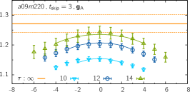
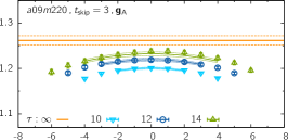
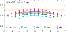
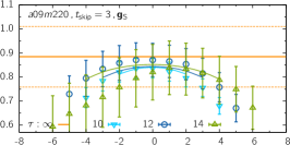
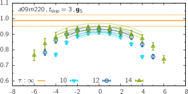
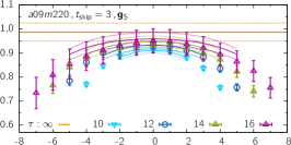
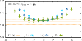
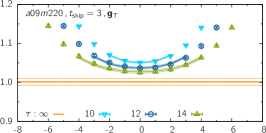
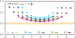
Figure 1: Illustration of the control over ESC in the isovector charges, $g_{A}^{u-d}$, $g_{S}^{u-d}$ and $g_{T}^{u-d}$, with higher statistics on the $a09m220$ ensemble. The left panels give the results based on 8000 HP measurements reported in Ref. Bhattacharya:2016zcn . The middle and right panels show new results with 123,392 AMA measurements. While the results from all three fits are consistent, the reliability of the fits, especially for $g_{S}^{u-d}$, is greatly improved when (i) the monotonic convergence in $\tau$ is manifest, and (ii) the fits and the values without (middle panels) and with (right panels) the $\mathop{t_{\rm sep}}\nolimits=16$ data overlap.

3 Simultaneous fit in $a$, $M_{\pi}$ and $M_{\pi}L$

Having calculated renormalized charges at various values of $a$, $M_{\pi}$ and $M_{\pi}L$, we perform a simultaneous fit to obtain results in the limit $a\to 0$, $M_{\pi}=135$ MeV and $M_{\pi}L\to\infty$. When fitting data given in Table 2 from the 10 HISQ ensembles, we include only the lowest order correction terms  Bhattacharya:2016zcn :

$$g_{A,S,T}^{u-d}(a,M_{\pi},L)=c_{1}+c_{2}a+c_{3}M_{\pi}^{2}+c_{4}M_{\pi}^{2}{e^{-M_{\pi}L}}\,.$$ (3)

Eq. (3) corrects a mistake made in Ref. Bhattacharya:2016zcn for the analysis of the isovector $g_{S}^{u-d}$. The leading chiral term is proportional to $M_{\pi}^{2}$ for the isovector case, and proportional to $M_{\pi}$ for the flavor diagonal cases.

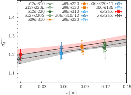
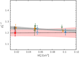
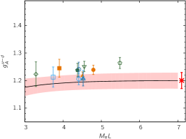
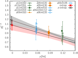
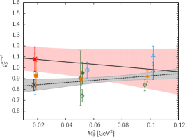
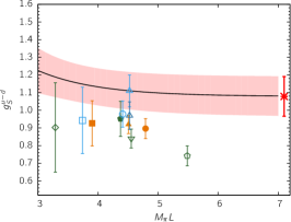
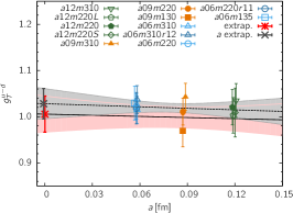
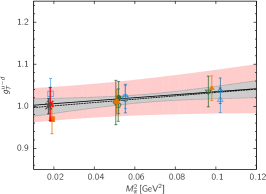
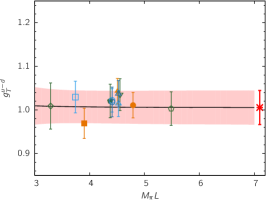
Figure 2: The 12-point fit using Eq. (3) to the data for the renormalized isovector charges $g_{A}^{u-d}$ and $g_{T}^{u-d}$ in the $\overline{{\rm MS}}$ scheme at $2\mathop{\rm GeV}\nolimits$, and the 11-point fit for $g_{S}^{u-d}$. (The $a06m220^{\ast}$ point is neglected as the 3-point data for $g_{S}^{u-d}$ are not monotonic in $\tau$.) The result of the simultaneous extrapolation to the physical point defined by $a\rightarrow 0$, $M_{\pi}\rightarrow M_{\pi^{0}}^{{\rm phys}}=135$ MeV and $L\rightarrow\infty$ are marked by a red star. The error bands in each panel are the result of a simultaneous fit but shown as a function of a single variable in the three panels. The overlay in the left (middle) panels with the dashed line within the grey band, is the fit to the data versus $a$ ($M_{\pi}^{2}$), i.e., neglecting dependence on the other two variables.

Fig. 2 shows that with reduced errors due to higher statistics data from 4 ensembles ($a12m220S$, $a12m220$, $a09m220$ and $a09m310$) and the addition of the second physical-mass ensemble $a06m135$, the behavior versus $a$, $M_{\pi}$ and $M_{\pi}L$ in the simultaneous fits is visibly clearer compared to the “9-point” fits presented in Ref. Bhattacharya:2016zcn . There is no significant evidence for finite volume corrections in any of the three charges for $M_{\pi}L>3.5$. There is some dependence of $g_{S}^{u-d}$ on $M_{\pi}^{2}$. The most evident trends are the positive slope versus $a$ in $g_{A}^{u-d}$ and the negative slope versus $a$ in $g_{S}^{u-d}$. Based on these fits shown in Fig. 2 and made using Eq. (3), our final estimates for the isovector charges, in the $\overline{\rm MS}$ scheme at 2 GeV, are:

$$g_{A}^{u-d} =1.20(3)\,,$$ (4)

$$g_{S}^{u-d} =1.08(11)\,,$$ (5)

$$g_{T}^{u-d} =1.01(4)\,.$$ (6)

Given the improved data and the fits in Fig. 2, the continued $2.5\sigma$ deviation of $g_{A}^{u-d}$ from the experimental value indicates that we are underestimating our errors. The largest change from results presented in Ref. Bhattacharya:2016zcn is the $1\sigma$ increase in the estimate of $g_{S}^{u-d}$. Most of this increase is due to correcting the form of the leading chiral term, i.e., $M_{\pi}\to M_{\pi}^{2}$, in Eq. (3). The major source of error in $g_{T}^{u-d}$ is now from the renormalization factor due to the poor convergence of the perturbative matching between the $\overline{\rm MS}$ and RI-sMOM schemes.

4 Comparison with CalLat Results for $g_{A}^{u-d}$

It is important to understand why our result for $g_{A}^{u-d}=1.20(3)$ presented in Eq. (6) differs from a similarly precise CalLat result $g_{A}^{u-d}=1.278(21)(26)$ that agrees with the experimental value $g_{A}^{u-d}=1.276(2)$ when the data shown in Table 2 on the 5 common ensembles are consistent. Our conclusion is that the majority of the difference comes from the final extrapolation in $a$. While we find a positive slope controlled by the data on the three $a=0.06$ fm ensembles, CalLat finds a negative slope anchored by the data on the coarser lattices. So the question is whether the differences in the two methods are manifest only at weaker couplng or are there systematic effects being missed in one or both calculations?

The two sets of calculations are being done on the same 2+1+1-flavor HISQ ensembles, but there are notable differences. These include: (i) Möbius domain wall versus clover for the valence quark action; (ii) gradient flow smearing with $t_{gf}/a=1$ versus one HYP smearing to smooth the lattices; (iii) different construction of the sequential propagator. CalLat inserts a zero-momentum projected axial current in all timeslices on the lattice simultaneously. This gives a summed contribution from all timeslices between and on the source and sink points plus all timeslices outside. CalLat thus uses a 2-state fit to $g_{A}=C_{3}(\tau+1)/C_{2}(\tau+1)-C_{3}(\tau)/C_{2}(\tau)$ to extract the charge where $C_{3}$ are 3-point functions with the insertion on all timeslices; (iv) CalLat report a much better statistical signal with fewer measurements.

The better statistical precision of the CalLat results for a given number of measurements is easy to understand: the CalLat fits to extract $g_{A}^{u-d}$ are based on a range of $\tau$ values that is shifted by 6–8 timeslices to smaller $\tau$ compared to our fit range. Since the errors in the data increase by a factor of two for every increase in $\tau$ by two lattice units, they gain a factor of up to $2^{4}$. Choosing values of $\tau$ within the range we have simulated, our estimates for the quantity they calculate, $g_{A}=C_{3}(\tau+1)/C_{2}(\tau+1)-C_{3}(\tau)/C_{2}(\tau)$, have similar errors. Note, also, that the CPU cost of the CalLat calculation is, ensemble by ensemble, higher because they simulate domain wall fermions and did not use the multigrid algorithm for propagator inversion.

The question, therefore, reduces to why their data can be fit starting at much smaller values of $\tau$? The correction due to ESC in their smeared-smeared data is less than $10\%$ even at $\tau\sim 3$ on the five common ensembles. The necessary condition to achieve this in our approach is reducing the overlap of the nucleon interpolating operator with the excited/multiparticle states to essentially zero. Since the source smearing used by the two collaborations is similar and the neutron interpolating operator is the same, the difference “must” come from the use of the gradient flow to smear the lattices. Further investigations are needed to confirm this interpretation (similar source smearing on gradient flow smoothed lattices produces sources with much smaller overlap with excited states) since one does not, a priori, expect the gradient flow smoothed lattices to change the overlap with the excited states, but only to reduce ultraviolet fluctuations.

5 Disconnected Contributions

We have calculated the disconnected contributions of light quarks on 5 ensembles $a12m310$, $a12m220$, $a09m310$, $a09m220$ and $a06m310$. For the strange quark we added the physical mass ensemble $a09m130$ and increased the statistics. The stocastic method used is the same as described in Ref. Bhattacharya:2015wna . The chiral-continuum plots for these data are shown in Fig. 3. The renormalization is carried out using the same factors as for isovector currents. While this has been shown to be a good approximation for $g_{A}$ and $g_{T}$ Green:2017keo , the same is not true for $g_{S}$. So the data for $g_{S}$ in Fig. 3 is shown only for completeness. Our estimates for the axial and tensor charges, after a simultaneous chiral-continuum extrapolation are:

$$g_{A}^{l} =-0.125(21)\qquad\qquad\ \ g_{A}^{s}=-0.065(12)\,,$$ (7)

$$g_{T}^{l} =\phantom{-}0.0042(79)\qquad\qquad g_{T}^{s}=\phantom{-}0.0043(34)\,.$$ (8)

Our new result $g_{T}^{s}=0.0043(34)$ is an improvement over the previously published value $g_{T}^{s}=0.008(9)$ Bhattacharya:2015wna . The result for $g_{T}^{l}$ is also still consistent with zero. Based on the current data, it is reasonable to assume that the magnitude of both after extrapolation is $\lesssim 0.01$. Therefore, to get a precise value will require higher precision data on more ensembles to improve the chiral-continuum extrapolation in $M_{\pi}^{2}$ and $a$. Given that we can bound their magnitude to be $\lesssim 0.01$, we will continue to neglect the disconnected compared to the connected contribution to $g_{T}^{u}$ and $g_{T}^{d}$ as discussed below.

These flavor diagonal tensor charges give the contribution of each quark’s electric dipole moment (qEDM) to the neutron EDM as discussed in Refs. Bhattacharya:2015esa ; Bhattacharya:2015wna . They are also probed in the measurements of transversity in deep inelastic scattering: the tensor charges are the integral over the longitudinal momentum fraction of the experimentally measured quark transversity distributions Ye:2016prn ; Bhattacharya:2015wna .

Results for the connected parts of the flavor diagonal charges, using the same renormalization factor as for the isovector currents, are

$$g_{A}^{u,{\rm conn}} =0.868(25)\qquad\qquad\ g_{A}^{d,{\rm conn}}=-0.331(16)\,,$$ (9)

$$g_{S}^{u,{\rm conn}} =4.78(29)\qquad\qquad\ \ \ g_{S}^{d,{\rm conn}}=\phantom{-}3.71(22)\,,$$ (10)

$$g_{T}^{u,{\rm conn}} =0.806(34)\qquad\qquad\ g_{T}^{d,{\rm conn}}=-0.203(14)\,.$$ (11)

Estimates for all three charges are consistent with those given in Ref. Bhattacharya:2015wna , and there is no significant reduction in the errors, which are still dominated by the final simultaneous chiral-continuum extrapolation.

Adding the connected and disconnected contributions for the axial charges and combining their errors in quadratures because the number of ensembles analyzed and the statistics are different in the two calculations, we get

$$g_{A}^{u} =0.743(33)\qquad\qquad g_{A}^{d}=-0.458(26)\qquad\qquad g_{A}^{s}=-0.065(12)\,,$$

$$g_{A}^{u,{\rm Expt.}} =0.843(12)\qquad\qquad g_{A}^{d,{\rm Expt.}}=-0.427(12)\,,$$ (12)

were we also give the experimental values Patrignani:2016xqp . There is a 2–3$\sigma$ difference between the lattice and experimental results for both $g_{A}^{u}$ and $g_{A}^{d}$. The analogous results for the neutron are given by the $u\leftrightarrow d$ interchange. From these axial charges, one gets the contribution of the quarks to the spin of the proton, $\Delta\Sigma_{q}/2=(g_{A}^{u}+g_{A}^{d}+g_{A}^{s})/2=0.11(5)$.

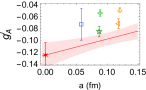
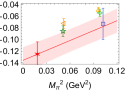
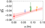
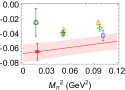
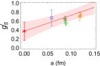
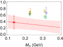
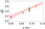
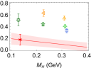
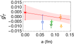
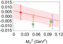
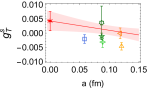
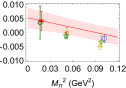
Figure 3: The continuum-chiral extrapolation for the contributions of the disconnected light (left 2 panels) and strange (right 2 panels) quarks. Each pair of panels shows the simultaneous fit versus $a$ and $M_{\pi}^{2}$ ($M_{\pi}$ for $g_{S}$), and the extrapolated value is marked with a red star. Possible finite volume corrections are neglected for lack of sufficient volume dependent data.

6 Summary

This talk presents the current status of our results for isovector and flavor diagonal charges of the nucleons using 10 ensembles of $2+1+1$-flavor HISQ ensembles generated by the MILC collaboration Bazavov:2012xda . The increase in statistics and the addition of a second physical mass ensemble has improved the fits, both to control excited state contamination as well as for the final chiral-continuum-finite volume extrapolation. Our estimate $g_{A}^{u-d}=1.20(3)$ is $2.5\sigma$ below the experimental value. We find deviations of similar size for the flavor diagonal charges $g_{A}^{u}$ and $g_{A}^{d}$. Results for the tensor charges are stable and the error in them is now dominated by the uncertainty in the renormalization factor. We have corrected an error in the form of the leading chiral correction used in the final simultaneous fit to the data for $g_{S}^{u-d}$, $M_{\pi}\to M_{\pi}^{2}$. As a result, the estimate for $g_{S}^{u-d}=1.08(11)$ is about $1\sigma$ larger than the value reported in Ref. Bhattacharya:2015wna . Our immediate goal is to double the statistics on the second physical mass ensemble $a06m135$ and finalize the analysis for publication.

Acknowledgement We thank the MILC Collaboration for providing the 2+1+1-flavor HISQ lattices and Emanuele Mereghetti for pointing out the correct form of the chiral correction in the isovector scalar charge. Simulations were carried out on computer facilities of (i) the USQCD Collaboration, which are funded by the Office of Science of the U.S. Department of Energy, (ii) the National Energy Research Scientific Computing Center, a DOE Office of Science User Facility supported by the Office of Science of the U.S. Department of Energy under Contract No. DE-AC02-05CH11231; (iii) Oak Ridge Leadership Computing Facility at the Oak Ridge National Laboratory, which is supported by the Office of Science of the U.S. Department of Energy under Contract No. DE-AC05- 00OR22725; (iv) Institutional Computing at Los Alamos National Laboratory; and (v) the High Performance Computing Center at Michigan State University. The calculations used the Chroma software suite Edwards:2004sx . This work is supported by the U.S. Department of Energy, Office of Science of High Energy Physics under contract number DE-KA-1401020 and the LANL LDRD program. The work of H-W. Lin was supported in part by the M. Hildred Blewett Fellowship of the American Physical Society.

References

- (1) T. Bhattacharya, V. Cirigliano, S. Cohen, R. Gupta, A. Joseph, H.W. Lin, B. Yoon (PNDME), Phys. Rev. D92, 094511 (2015), 1506.06411
- (2) T. Bhattacharya, V. Cirigliano, R. Gupta, H.W. Lin, B. Yoon, Phys. Rev. Lett. 115, 212002 (2015), 1506.04196
- (3) T. Bhattacharya, V. Cirigliano, S. Cohen, R. Gupta, H.W. Lin, B. Yoon, Phys. Rev. D94, 054508 (2016), 1606.07049
- (4) A. Bazavov et al. (MILC Collaboration), Phys.Rev. D87, 054505 (2013), 1212.4768
- (5) Y. Jang et al., ibid (2016)
- (6) E. Berkowitz et al. (2017), 1704.01114
- (7) J. Green, N. Hasan, S. Meinel, M. Engelhardt, S. Krieg, J. Laeuchli, J. Negele, K. Orginos, A. Pochinsky, S. Syritsyn, Phys. Rev. D95, 114502 (2017), 1703.06703
- (8) Z. Ye, N. Sato, K. Allada, T. Liu, J.P. Chen, H. Gao, Z.B. Kang, A. Prokudin, P. Sun, F. Yuan, Phys. Lett. B767, 91 (2017), 1609.02449
- (9) C. Patrignani et al. (Particle Data Group), Chin. Phys. C40, 100001 (2016)
- (10) R.G. Edwards, B. Joo (SciDAC Collaboration, LHPC Collaboration, UKQCD Collaboration), Nucl.Phys.Proc.Suppl. 140, 832 (2005), hep-lat/0409003