Existence and continuity of solution trajectories of generalized equations with application in electronics

Abstract.

We consider a special form of parametric generalized equations arising from electronic circuits with AC sources and study the effect of perturbing the input signal on solution trajectories. Using methods of variational analysis and strong metric regularity property of an auxiliary map, we are able to prove the regularity properties of the solution trajectories inherited by the input signal. Furthermore, we establish the existence of continuous solution trajectories for the perturbed problem. This can be achieved via a result of uniform strong metric regularity for the auxiliary map.

1. Introduction

This paper deals with parametric generalized equations of the form

$$0\in f(x)-p(t)+F(x),$$ (1)

where $f:\mathbb{R}^{n}\longrightarrow\mathbb{R}^{n}$ is a (usually) smooth function, $p:\mathbb{R}\longrightarrow\mathbb{R}^{n}$ is a function of parameter $t\in[0,1]$, and $F:\mathbb{R}^{n}\rightrightarrows\mathbb{R}^{n}$ is a set-valued map with closed graph.
Generalized equations (when $p$ is a constant function) has been well studied in the literature of variational analysis (see, for instance, [implicit, Mordukhovich] and references therein). Robinson in [robinson1979generalized, robinson1982generalized, robinson1983generalized, robinson] studied in details the case where $F$ is the normal cone at a point $x\in\mathbb{R}^{n}$ (in the sense of convex analysis) to a closed and convex set, and found the setting of generalized equations as an appropriate way to express and analyse problems in complementarity systems, mathematical programming, and variational inequalities.
In recent years, the formalism of generalized equations has been used to describe the behaviour of electronic circuits ([adly2, adly, adly3]). In the study of electrical circuits, power supplies (that is, both current and voltage sources) play an important role. Not only their failure in providing the minimum voltage level for other components to work would be a problem, but also small changes in the provided voltage level will affect the whole circuit and the goal it has been designed for. These small changes around a desired value could happen mainly because of failure in precise measurements, ageing process, and thermal effects (see [Iman2017, Sedra]). Thus, based on the type of voltage/current sources in the circuits, two different cases may be considered:

1. static case:
   This is the situation when the signal sources in the circuit are DC (that is, their value is not changing with respect to time). For practical reasons, we would prefer to rewrite (1) as $p\in f(x)+F(x)$, where $p\in\mathbb{R}^{n}$ is a fixed vector representing the voltage or current sources in the circuit, and $x\in\mathbb{R}^{n}$ represents the mixture of $n$ variables which are unknown currents of branches or voltages of components. The corresponding solution mapping can be defined as follows:

   $$p\longmapsto S(p):=\left\{x\in\mathbb{R}^{n}~{}|~{}p\in f(x)\,+F(x)\right\}.$$ (2)

   In this framework, small deviations of $x$ with respect to perturbations of $p$ around a presumed point $(\bar{p},\bar{x})\in\mathrm{gph}\,S$ could be formulated in terms of local stability properties of $S$ at $\bar{p}$ for $\bar{x}$. Providing some first order and second order criteria to check the local stability properties of a set-valued map has been the subject of many papers [adly2, adly, durea2012openness, Mordukhovich] to mention a few.

2. dynamic case:
   When an AC signal source (that is, its value is a function of time) is in the circuit, the problem could be more complicated. First of all, the other variables of the model would become a function of time, too. Second, it is not appropriate any more to formulate the solution mapping as $S(p)$. One can consider a parametric generalized equation like (1) where $p$ now depends on a scalar parameter $t\in[0,1]$, and define the corresponding solution mapping as

   $$S:t\mapsto S(t)=\{x\in\mathbb{R}^{n}~{}|~{}-p(t)+f(x)+F(x)\ni 0\}.$$ (3)

   The third difficulty rises here: the study of the effects of perturbations of $p$ is not equivalent any more to searching the local stability properties of $S$.
   Clearly, in this framework for any fixed $t\in[0,1]$ one has a static case problem. This approach is well known and well studied in the literature, both as a pointwise study (see for instance [Mordukhovich, Bianchi2013279, Artacho20101149, uderzo2009some] and references therein), or as a numerical method and for designing algorithms (see for example [ferreira2016kantorovich, ferreira2016unifying, dontchev2010newton, adly2016newton, adly2015newton]). In this paper, instead of looking at the sets $S(t)$, we focus on solution trajectories, functions like $x:[0,1]\to\mathbb{R}^{n}$ such that $x(t)\in S(t),\mathrm{~{}~{}~{}~{}for~{}all~{}}t\in[0,1]$, that is, $x(\cdot)$ is a selection for $S$ over $[0,1]$.

The main aim of this paper is to investigate the dependence of the solution trajectories on the regularity and changes of the input signal $p$. A side goal is to develop a relationship between pointwise stability properties and their “uniform” version. This has been done with reference to the property of strong metric regularity.
The paper is organized as follows: In Section 2, we provide the preliminary definitions. in Section 3, we give the sketch of the mathematical model for perturbation study of the input signal in the circuits. In Section 4, which contains the main contributions of this paper, we answer questions related to the existence of selections which are regular functions, their relationship with the input signal (Subsection 4.1), and their reaction to the small perturbations of the input signal (Subsection LABEL:Perturbations_of_the_Input_Signal). We also extend a previous result in [dontchev2013] about uniform strong metric regularity with respect to $t$ over an interval in Subsection LABEL:Uniform_Strong_Metric_Regularity-subsection.

2. Preliminaries

In working with $\mathbb{R}^{n}$ we will denote by $\|x\|$ the Euclidean norm associated with the canonical inner product. The closed ball around $\bar{x}$ with radius $r$ is $\mathbb{B}_{r}(\bar{x})=\{x\in\mathbb{R}^{n}~{}|~{}~{}\|x-\bar{x}\|\leq r\}$, where the open ball is denoted by int $\mathbb{B}_{r}(\bar{x})$. We denote the closed unit ball $\mathbb{B}_{1}(0)$ by $\mathbb{B}$.
The graph, domain, and range of a given set-valued map $F:\mathbb{R}^{n}\rightrightarrows\mathbb{R}^{m}$ are defined, respectively, by gph $F:=\{(x,y)\in\mathbb{R}^{n}\times\mathbb{R}^{m}~{}|~{}x\in\mathbb{R}^{n}~{},~{}y\in F(x)\}$, dom $F:=\{x\in\mathbb{R}^{n}~{}|~{}F(x)\neq\emptyset\}$, and rge $F:=\{y\in\mathbb{R}^{m}~{}|~{}y\in F(x)~{}~{}\mathrm{for~{}some}~{}x\in\mathbb{R}^{n}\}$.
A mapping $S:\mathbb{R}^{m}\rightrightarrows\mathbb{R}^{n}$ is said to have the Aubin property at $\bar{y}\in\mathbb{R}^{m}$ for $\bar{x}\in\mathbb{R}^{n}$ if $\bar{x}\in S(\bar{y})$, the graph of $S$ is locally closed at $(\bar{y},\bar{x})$, and there is a constant $\kappa\geq 0$ together with neighborhoods $U$ of $\bar{x}$ and $V$ of $\bar{y}$ such that

$$e(S(y^{\prime})\cap U,S(y))\leq\kappa~{}\|y^{\prime}-y\|\mathrm{~{}~{}~{}for~{}all~{}~{}}y^{\prime},y\in V,$$ (4)

where $e(A,B)$ is the excess of $A$ beyond $B$ defined as

$$e\,(A,B):=\sup_{x\in A}d(x,B)=\sup_{x\in A}\,\inf_{y\in B}d(x,y).$$ (5)

The infimum of $\kappa$ over all such combinations of $\kappa,U,$ and $V,$ is called the Lipschitz modulus of $S$ at $\bar{y}$ for $\bar{x}$ and is denoted by lip $(S;\bar{y}|\bar{x})$.
$S$ is said to be calm at $\bar{y}$ for $\bar{x}$ if $(\bar{y},\bar{x})\in\mathrm{gph}\,S$, and there is a constant $\kappa\geq 0$ along with neighborhoods $U$ of $\bar{x}$ and $V$ of $\bar{y}$ such that

$$e(S(y)\cap U,S(\bar{y}))\leq\kappa~{}\|y-\bar{y}\|\mathrm{~{}~{}~{}~{}for~{}all~{}}y\in V.$$ (6)

The infimum of $\kappa$ over all such combinations of $\kappa$, $U$ and $V$ is called the calmness modulus of $S$ at $\bar{y}$ for $\bar{x}$ and is denoted by clm $(S;\bar{y}|\bar{x})$.
A mapping $S$ is said to have the isolated calmness property if it is calm at $\bar{y}$ for $\bar{x}$ and, in addition, $S$ has a graphical localization at $\bar{y}$ for $\bar{x}$ that is single-valued at $\bar{y}$ itself (with value $\bar{x}$). Specifically, this refers to the existence of a constant $\kappa\geq 0$ and neighborhoods $U$ of $\bar{x}$ and $V$ of $\bar{y}$ such that

$$\|x-\bar{x}\|~{}\leq\kappa~{}\|y-\bar{y}\|\mathrm{~{}~{}~{}~{}when~{}}x\in S(y)\cap U\mathrm{~{}~{}and~{}~{}}y\in V.$$ (7)

A mapping $F:\mathbb{R}^{n}\rightrightarrows\mathbb{R}^{m}$ is said to be metrically regular at $\bar{x}$ for $\bar{y}$ when $\bar{y}\in F(\bar{x})$, the graph of $F$ is locally closed at $(\bar{x},\bar{y})$, and there is a constant $\kappa\geq 0$ together with neighborhoods $U$ of $\bar{x}$ and $V$ of $\bar{y}$ such that

$$d\big{(}x,F^{-1}(y)\big{)}\leq\kappa~{}d(y,F(x))\mathrm{~{}~{}~{}whenever~{}~{}}(x,y)\in U\times V.$$ (8)

The infimum of $\kappa$ over all such combinations of $\kappa$, $U$ and $V$ is called the regularity modulus of $F$ at $\bar{x}$ for $\bar{y}$ and is denoted by reg $(F;\bar{x}|\bar{y})$.
A mapping $F$ with $(\bar{x},\bar{y})\in\mathrm{gph}\,F$ whose inverse $F^{-1}$ has a Lipschitz continuous single-valued localization around $\bar{y}$ for $\bar{x}$ will be called strongly metrically regular (SMR for short) at $\bar{x}$ for $\bar{y}$. Indeed, strong metric regularity is just metric regularity plus the existence of a single-valued localization of the inverse (see [implicit, Proposition 3G.1, p. 192]).
$F$ is called metrically sub-regular at $\bar{x}$ for $\bar{y}$ if $(\bar{x},\bar{y})\in\mathrm{gph}\,F$ and there exists $\kappa\geq 0$ along with neighborhoods $U$ of $\bar{x}$ and $V$ of $\bar{y}$ such that

$$d(x,F^{-1}(\bar{y}))~{}\leq~{}\kappa\,d(\bar{y},F(x)\cap V)\mathrm{~{}~{}~{}~{}for~{}all~{}}x\in U.$$ (9)

The infimum of all $\kappa$ for which (9) holds is the modulus of metric sub-regularity, denoted by $\mathrm{subreg\,}(F;\bar{x}|\bar{y})$. Finally, $F$ is said to be strongly metrically sub-regular at $\bar{x}$ for $\bar{y}$ if $(\bar{x},\bar{y})\in\mathrm{gph}\,F$ and there is a constant $\kappa\geq 0$ along with neighborhoods $U$ of $\bar{x}$ and $V$ of $\bar{y}$ such that

$$\|x-\bar{x}\|\leq\,\kappa\,d(\,\bar{y},\,F(x)\cap V)~{}\mathrm{~{}~{}~{}~{}for~{}all~{}}x\in U.$$ (10)

For a function $f:\mathbb{R}^{d}\times\mathbb{R}^{n}\longrightarrow\mathbb{R}^{m}$ and a point $(\bar{p},\bar{x})\in\mathrm{int~{}dom}\,f$, a function $h:\mathbb{R}^{n}\longrightarrow\mathbb{R}^{m}$ is said to be an estimator of $f$ with respect to $x$ uniformly in $p$ at $(\bar{p},\bar{x})$ with constant $\mu$ if $h(\bar{x})=f(\bar{p},\bar{x})$ and $\widehat{\mathrm{clm}}_{x}\,(e;(\bar{p},\bar{x}))\leq\mu<\infty$ for $e(p,x)=f(p,x)-h(x)$, where $\widehat{\mathrm{clm}}_{x}$ is the uniform partial calmness modulus

$$\widehat{\mathrm{clm}}_{x}\,(e;(\bar{p},\bar{x})):=\limsup_{\mathclap{\begin{subarray}{c}x\rightarrow\bar{x},p\rightarrow\bar{p}\\ (p,x)\,\in\,\mathrm{dom}\,e,x\not=\bar{x}\end{subarray}}}\dfrac{\|e(p,x)-e(p,\bar{x})\|}{\|x-\bar{x}\|}.$$

It is a strict estimator in this sense if the stronger condition holds that

$$\widehat{\mathrm{lip}}_{x}\,(e;(\bar{p},\bar{x}))\leq\mu<\infty~{}~{}\mathrm{~{}~{}~{}~{}~{}~{}~{}~{}~{}for~{}~{}}e(p,x)=f(p,x)-h(x),$$

and similarly, $\widehat{\mathrm{lip}}_{x}$ is the uniform partial Lipschitz modulus. In the case of $\mu=0$, such an estimator is called a partial first-order approximation.

3. Modelling

In this section we will briefly present the practical problem we would face thorough the paper and provide the appropriate mathematical models for it.
An electrical circuit is made of some electrical (or electronic) components connected together in a special way with wires to serve a specific duty. For describing a component $Z$, we would look at the current passing through it, referred to as $i_{Z}$ and the electric potential difference between its terminals, that is voltage over it, referred to as $v_{Z}$.
The behaviour of the component under different voltages and various currents is usually described with a graph in the $i-v$ plane, and referred to as the $i-v$ characteristic of the component. These graphs could be presented with functions, like the resistors with the linear relation $v_{R}=Ri_{R}$ (where $R>0$ is a fixed number called Resistance), or set-valued maps, like Diodes.
Based on the components in the circuit, and the exactness of the solution required, there is a huge theory and lots of work done around it till now, in electrical engineering literature. We are not exactly interested in this topic, but we will use the setting and rules of circuit theory to formulate our problem.

3.1. Static case.

We start with a simple circuit as shown below (Figure 1) which involves a Zener Diode. Our aim is to find a relation between the given input voltage ($E$, here) and the variable $I$, current, in the circuit using the Kirchoff’s voltage and current laws.

        

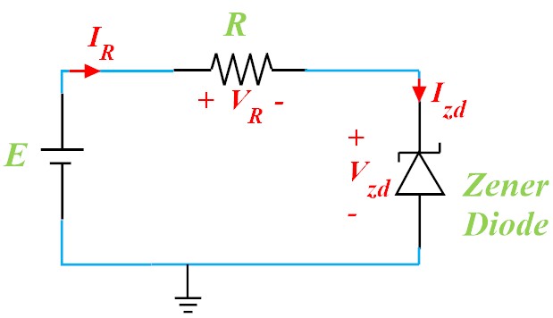
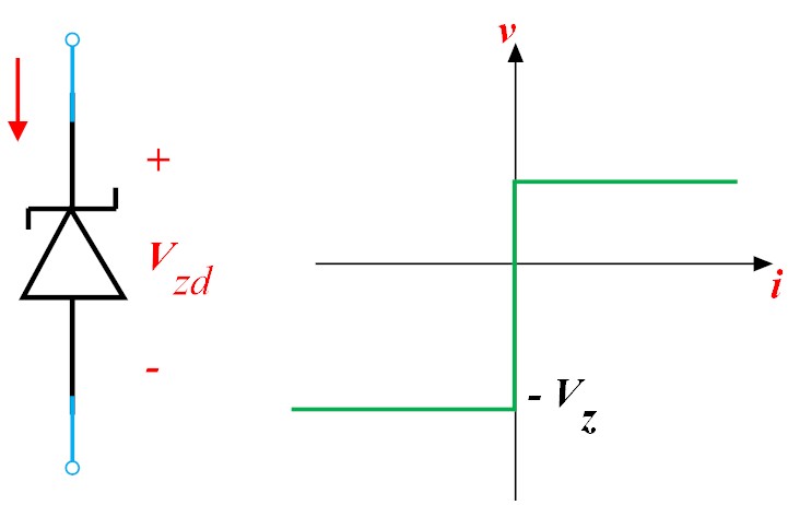
Figure 1. A simple electrical circuit, the schematic and $i-v$ characteristic of Zener Diode

$$\left.\begin{matrix}\mathrm{KVL:}&-E+V_{R}+V_{zd}=0~{}\\ \mathrm{KCL:}&I_{R}=I_{zd}=I~{}~{}~{}~{}~{}~{}~{}~{}\\ ~{}~{}&V_{R}=R\,I_{R}\\ ~{}~{}&V_{zd}\in F(I_{zd})\end{matrix}\right\}~{}~{}\Rightarrow~{}~{}~{}E\in R\,I~{}+F(I),$$ (11)

in which $F(I)$ describes the relation between $I_{zd}$ and $V_{zd}$ as the set-valued map given by the $i-v$ characteristic of the diode. Let us change $E$ to $p$, in order to indicate that it is a parameter; and $I$ to $z$, to show that $z$ is the variable, thus we get

$$p\in f(z)+F(z),$$ (12)

in which $f(z)=R\,z$, in this particular example. For a given $p$, we are interested in the solution mapping defined as $S(p)=\left\{z\in\mathbb{R}~{}|~{}p\in f(z)+F(z)\right\}$.
Regarding different electronic components in the circuit and various circuit schematics, one might need to use some correction matrices to differ those branches that have diodes from others. The general form of the solution mapping in this case would be

$$\begin{matrix}\Phi(z):=f(z)\,+BF(Cz)\\ S(p):=\big{\{}z\in\mathbb{R}^{n}~{}|~{}p\in\Phi(z)\big{\}},~{}\end{matrix}$$ (13)

where $p\in\mathbb{R}^{n}$ is a fixed vector, $f:\mathbb{R}^{n}\longrightarrow\mathbb{R}^{n}$ is a function, and $F:\mathbb{R}^{m}\rightrightarrows\mathbb{R}^{m}$ is a set-valued map (with certain assumptions), and $B\in\mathbb{R}^{n\times m},~{}C\in\mathbb{R}^{m\times n}$ are given matrices.
We are going to answer the question concerning the change of source voltage from $\bar{p}$ to $p^{\prime}$. We try to provide an interpretation of the local stability properties of the solution mapping in terms of the circuit parameters. Let us note that based on the problem one may face during the design process, one of these properties would fit better to his/her demands.

Stability Formulation. Suppose that for a given $\bar{p}$, we know the previous current of operating point, say $\bar{z}$. We also assume that the input change is small, that is, in mathematical terms, $p^{\prime}\in\mathbb{B}_{r}(\bar{p})=:V$ for some small $r>0$.
We are interested in those circuits that keep the small input-change, small. More precisely, the distance between a $z\in S(p^{\prime})$ and $\bar{z}$, is controlled by the distance $\|~{}p^{\prime}-\bar{p}~{}\|$. Thus we wish (and search for) $S$ having the following property

$$\|~{}z-\bar{z}~{}\|\,\leq\,\kappa~{}\|~{}p^{\prime}-\bar{p}~{}\|~{}~{}\mathrm{~{}~{}when~{}~{}~{}}~{}z\in S(p^{\prime})\cap U,~{}~{}p^{\prime}\in V$$ (14)

where $U$ is a neighborhood of $\bar{z}$, $V$ is a neighborhood of $\bar{p}$, and $\kappa\geq 0$ is a constant. This property has already been introduced as isolated calmness.
The reason we considered the intersection $S(p^{\prime})\cap U$ in the above formulation, is that while it is possible to have different values in $S(p^{\prime})$, we are just interested in quarantining the existence of a $z$ near enough to $\bar{z}$.
$S$ may be not single-valued at $p^{\prime}$, hence, with a slight modification of the previous formulation, one can obtain the property of calmness as defined in (6). If we are investigating a general local property of the solution mapping and the point $(\bar{p},\bar{z})\in\mathrm{gph}\,S$ does not play a crucial role in our study, we would be interested in the “two-variable” version of the previous condition, and hence search for the Aubin property (4).

Regularity Formulation. Up to now, the construction has been built under the assumption that the explicit form of the solution mapping $S(\cdot)$ is in hand and so we can easily calculate values like $S(p^{\prime})$, which is not true in general. All we are sure we can get from the circuit is $\Phi=S^{-1}$. It is not always simple (or even possible) to derive the formula of $S$, so we need to provide the proper formulation of the desired properties with $\Phi$.
One can start from a point $(\bar{z},\bar{p})\in\mathrm{gph}\,\Phi$, take an arbitrary $z^{\prime}\in U=:\mathbb{B}_{r_{1}}(\bar{z})$, calculate $\Phi(z^{\prime})$, take a $p\in V=:\mathbb{B}_{r_{2}}(\bar{p})$, and then ask for the chance of having the output distance $d\left(z^{\prime},\Phi^{-1}(p)\right)$ being controlled by the input distance $d\left(p,\Phi(z^{\prime})\right)$, that is,

$$d\left(z^{\prime},\Phi^{-1}(p)\right)\leq\kappa~{}d\left(p,\Phi(z^{\prime})\right)\mathrm{~{}~{}~{}whenever~{}~{}}(z^{\prime},p)\in U\times V,$$ (15)

which is introduced as metric regularity (8).
Then, make slight modifications by considering the additional condition of single-valuedness at $\bar{z}$ (that is, demanding strong metric regularity); or considering the one-variable version of the above condition (introduced as metric sub-regularity). The relations that hold between the local stability and metric regularity properties of an arbitrary set-valued map have been well studied in the literature [implicit].
Let us note that if $f$ is not smooth, one can face the problem by means of generalized derivatives as in [izmailov2014, cibulka2016strong].

3.2. Dynamic case.

Let us start with an example. In Figure 2, a simple regulator circuit with a practical model for the diode is shown. The voltage source is made of $n$ batteries connected to each other in a serial scheme, that provides $n+1$ different levels between $0\,V_{s}$, and $1\,V_{s}$.

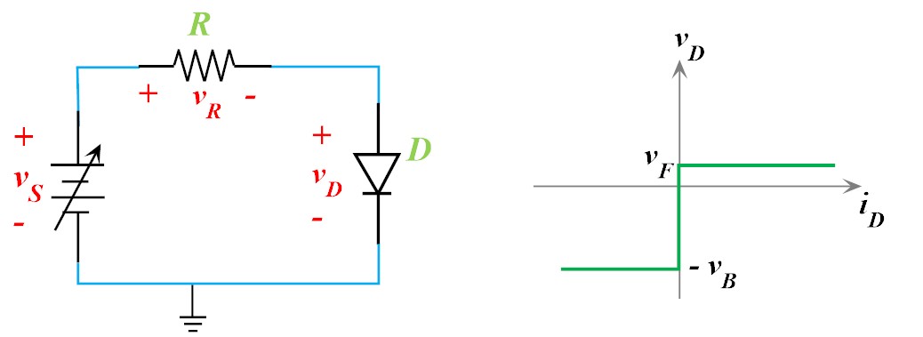
Figure 2. A regulator circuit with multiple DC sources

Using Kirchhoff’s laws and $i-v$ characteristics of diode and resistor, we obtain that:

$$\left.\begin{matrix}\mathrm{KVL:}&-\frac{m}{n}V_{S}+V_{R}+V_{D}=0~{}\\ \mathrm{KCL:}&I_{D}=I_{R}=:I~{}~{}~{}~{}~{}~{}~{}~{}~{}~{}~{}\\ ~{}~{}~{}~{}&\,V_{R}=R\,I_{R}~{}~{}~{}~{}~{}~{}~{}~{}~{}~{}\\ ~{}~{}~{}~{}&\,V_{D}\in F(I_{D})~{}~{}~{}~{}~{}~{}~{}~{}\\ \end{matrix}\right\}~{}~{}\Rightarrow\quad 0\in-p+Rz+F(z),$$ (16)

where $p=\frac{m}{n}V_{S}$, $z=I$, and $m=0,1,\,\dots,n$, indicates the number of turned-on batteries in the circuit. Then, the solution mapping would be

$$S(p)=\{\,z\in\mathbb{R}\,|\,-p+Rz+F(z)\ni 0\,\}.$$

In order to find $S(p)$, we can consider the three parts of $\mathrm{gph}\,F$ separately to solve the generalized equation, fortunately, analytically this time.

1. For $z>0$, with $F(z)=\{v_{F}\}$.
   Then, we would have an equation, $-p+Rz+v_{F}=0$. Thus, $z=\dfrac{p-v_{F}}{R}$ which is only valid for $z>0$, that is, when $p>v_{F}$.

2. For $z=0$, with $F(z)=[-v_{B},v_{F}]$.
   Then, $-p+0+[-v_{B},v_{F}]\ni 0$. That is, $z=0$ for $p\in[-v_{B},v_{F}]$.

3. For $z<0$, with $F(z)=\{-v_{B}\}$.
   Then, again we would have an equation, $-p+Rz-v_{B}=0$. Thus, $z=\dfrac{p+v_{B}}{R}$, as long as $p<-v_{B}$.

Therefore, $S$ is a single-valued map in this problem, with the graph shown in Figure 3 (left), and the rule given as:

$$S(p)=\left\{\begin{matrix}~{}\Big{\{}\dfrac{p+v_{B}}{R}\Big{\}}&&p<-v_{B}\\ &&\\ ~{}\Big{\{}0\Big{\}}&&~{}~{}~{}~{}~{}~{}~{}p\in[-v_{B},v_{F}]\\ &&\\ ~{}\Big{\{}\dfrac{p-v_{F}}{R}\Big{\}}&&p>v_{F}\end{matrix}\right.$$ (17)

When we deal with an AC voltage source, theoretically we can follow the same procedure. For any $t\in[0,1]$, use the specific value $p(t)$ and the transformation graph to find the value of $z$ at that time, that is $z(t)$. Then, we can obtain the graph of $z(\cdot)$ with respect to time, similar to the one shown in Figure 3 (right) for a sinusoid signal.
There are two interesting facts to highlight here:

1. Very naturally, instead of asking for the graph of the solution mapping with respect to the input signal, we focused on the graph of the solution mapping with respect to the time. Of course, when the solution mapping is not a function like this problem, the latter expression needs a clarification.

2. Dealing with a function as the input signal, we searched for a function as the output signal. In order to keep the notations consistent, yet without ambiguity, we will refer to these functions as $p(\cdot)$, $p:\mathbb{R}\longrightarrow\mathbb{R}^{n}$, $z(\cdot)$, and so on.

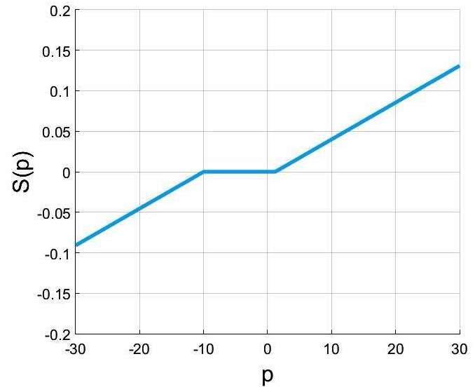
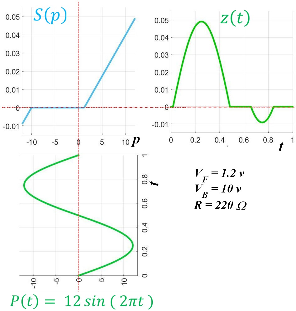
Figure 3. Solution mapping for the circuit in Figure 2 (left), graphical method to find the output for a typical input (right)

Therefore, in the case of time varying sources, we can assume that $t$ is a parameter, it belongs to a set like $[0,1]$, and it would be more appropriate to consider the solution mapping as the (generally set-valued) map that associates to every $t\in[0,1]$, the set of all possible vectors $z$ in $\mathbb{R}^{n}$ that fits the generalized equation

$$f(z)-p(t)+F(z)\ni 0.$$ (18)

The solution mapping is therefore given by

$$S:t\mapsto S(t)=\{z\in\mathbb{R}^{n}~{}|~{}f(z)-p(t)+F(z)\ni 0\},$$ (19)

and a solution trajectory over $[0,1]$ is, in this case, a function $\bar{z}(\cdot)$ such that $\bar{z}(t)\in S(t)$ for all $t\in[0,~{}1]$, that is, $\bar{z}(\cdot)$ is a selection for $S$ over $[0,1]$.
Defining the solution mapping in terms of the parameter $t$, and not directly of the input signal $p$, will cause some difficulties to study the perturbation problem.
Comparing to the static case, although for each $t$ one needs to solve a generalized equation of the type discussed in depth in equation (13), the Aubin property of the solution mapping at a certain point is not sufficient any more to guarantee the stability of the output with respect to the perturbations of the input signal. In other words, the relation between $S$ and $p(\cdot)$ is not explicitly expressed now.
Let us note that when $p$ is a continuous function and under the general assumptions:

1. $f$ is continuously differentiable in $\mathbb{R}^{n}$;

2. $F$ has closed graph;

the map $S$ has closed graph. Consider a function $h:\mathbb{R}\times\mathbb{R}^{n}\longrightarrow\mathbb{R}^{n}$, defined as $h(t,v)=-p(t)+f(v)$. Then, the generalized equation (18) can be written as

$$h(t,v)+F(v)\ni 0.$$ (20)

For any given $(t,z)\in\mathrm{gph}\,S$, define the mapping

$$v\mapsto G_{t,z}(v):=h(t,z)+\nabla_{z}h(t,z)\,(v-z)+F(v).$$ (21)

A point $(t,z)\in\mathbb{R}^{1+n}$ is said to be a strongly regular point (see Robinson [robinson]) for the generalized equation (18, or equivalently, 20) when $(t,z)\in\mathrm{gph}\,S$ and the mapping $G_{t,z}$ is strongly metrically regular at $z$ for $0$. That is, there exist constants $a_{t},~{}b_{t},~{}\lambda_{t}>0$ such that the mapping

$$\mathbb{B}_{b_{t}}(0)\ni y\longmapsto G_{t,z}^{-1}(y)\cap\mathbb{B}_{a_{t}}(z(t))$$ (22)

is a Lipschitz continuous function with a Lipschitz constant $\lambda_{t}$.
From [implicit, Theorem 2B.7, p. 89], one obtains that when $(\bar{t},\bar{z})$ is a strongly regular point for (18), there are open neighborhoods $T$ of $\bar{t}$ and $U$ of $\bar{z}$ such that the mapping

$$T\cap[0,1]\ni\tau\mapsto S(\tau)\cap U$$ (23)

is single-valued and Lipschitz continuous on $T\cap[0,~{}1]$. Then, [implicit, Theorem 6G.1, p. 426] shows that if each point in $\mathrm{gph}\,S$ is strongly regular, then there are finitely many Lipschitz continuous solution trajectories defined on $[0,1]$ whose graphs never intersect each other. In addition, along any such trajectory $\bar{u}(\cdot)$ the mapping $G_{t,\bar{u}(t)}$ is strongly regular uniformly in $t\in[0,1]$, meaning that the neighborhoods and the constants involved in the definition do not depend on $t$. Although this theorem is an important result in our study, there is an unpleasant assumption there: $S(t)$ is uniformly bounded. Even if this condition is fulfilled, it is hard to be checked since it requires the whole set $S(t)$ to be clarified and available for any $t\in[0,1]$. In the next section it will be shown that the uniform bound could be obtained without this extra assumption.

4. Time-varying case

In this sections we will focus on the problem that is modelled with equations (18 - 21). Although we are inspired by Robinson’s idea of strongly regular points in defining the auxiliary map (21), and the techniques in [implicit, Theorems 2B.7, 5G.3, and 6G.1], we find it more convenient to do some modifications in the setting in order to adapt it to our problem.
Since our aim in this section is the study of the solution trajectories with respect to variations of the input function, $p(t)$, and since working with the function $f(z)$ or with its first order approximation does not play an important role in our case (the proof of this statement will follow soon), we assume to deal with $f(z)$ itself and so to consider the auxiliary mapping

$$v\mapsto G_{t}(v):=f(v)-p(t)+F(v).$$ (24)

For more details on different possible choices of auxiliary maps and how the strong metric regularity would be affected, we state the following proposition:

Proposition 4.1 (Different Auxiliary Maps).

Suppose that $F:\mathbb{R}^{n}\rightrightarrows\mathbb{R}^{n}$ is a set-valued map with closed graph, and $f:\mathbb{R}\times\mathbb{R}^{n}\longrightarrow\mathbb{R}^{n}$ is a function admitting $h$ as a strict estimator with respect to $u$ uniformly in $t$, at $(\bar{t},\bar{u})$ with a constant $\mu$. Given the generalized equation $f(t,u)+F(u)\ni 0$, consider the following auxiliary maps:

$$G_{\bar{t},\bar{u}}(v)=h(v)+F(v),\,$$ (25)

$$G_{\bar{t}}(v)=f(\bar{t},v)+F(v).$$ (26)

Then, $G_{\bar{t},\bar{u}}$ is SMR at $\bar{u}$ for $0$, if and only if $G_{\bar{t}}$ is SMR at $\bar{u}$ for $0$, provided that the conditions $\mu\,\mathrm{reg}\,(G_{\bar{t},\bar{u}}\,;\,\bar{u})<1$, and $\mu\,\mathrm{reg}\,(G_{\bar{t}}\,;\,\bar{u})<1$ holds.

Proof. First observe that, by definition of a strict estimator, $h(\bar{u})=f(\bar{t},\bar{u})$ and so, $0\in G_{\bar{t},\bar{u}}(\bar{u})$ is equivalent to $0\in G_{\bar{t}}(\bar{u})$. Now taking into account the pointwise relation

$$G_{\bar{t}}(v)=f(\bar{t},v)+F(v)=G_{\bar{t},\bar{u}}(v)+f(\bar{t},v)-h(v),$$

one can define a map $g_{\bar{t},\bar{u}}:\mathbb{R}^{n}\longrightarrow\mathbb{R}^{n}$ with $g_{\bar{t},\bar{u}}(v)=f(\bar{t},v)-h(v)$. For any $v_{1},v_{2}\in U$ (a neighborhood of $\bar{u}$), we get

$$\begin{split}\left\|g_{\bar{t},\bar{u}}(v_{1})-g_{\bar{t},\bar{u}}(v_{2})\right\|&=\left\|f(\bar{t},v_{1})-h(v_{1})-f(\bar{t},v_{2})+h(v_{2})\right\|\\ &=\left\|e(\bar{t},v_{1})-e(\bar{t},v_{2})\right\|\\ &\leq\mu\left\|v_{1}-v_{2}\right\|\end{split}$$

where the last inequality is obtained by definition of strict estimator. Thus, $g_{\bar{t},\bar{u}}$ is Lipschitz continuous around $\bar{u}$.
Now one can use [implicit, Theorem 2B.8, p. 89] with $G=G_{\bar{t},\bar{u}}$ and $g=g_{\bar{t},\bar{u}}$ and, by assuming that $\mu\,\mathrm{reg}\,(G_{\bar{t},\bar{u}}\,;\,\bar{u})<1$, to conclude that $g+G=G_{\bar{t}}$ has a Lipschitz continuous single-valued localization around $0+g(\bar{u})$ for $\bar{u}$. Since $g_{\bar{t},\bar{u}}(\bar{u})=h(\bar{u})-f(\bar{t},\bar{u})=0$, the latter could be expressed as the SMR of $G_{\bar{t}}$ at $\bar{u}$ for $0$.
The converse implication is satisfied in a similar way by letting $G=G_{\bar{t}}$, $g=-g_{\bar{t},\bar{u}}$ and assuming $\mu\,\mathrm{reg}\,(G_{\bar{t}}\,;\,\bar{u})<1$. $\Box$

Remark 4.2.

(a) A closer look at the proof reveals that if $h$ is a strict estimator, then the regularity modulus of $G_{\bar{t}}$ and $G_{\bar{t},\bar{u}}$ are related to each other with $\kappa^{\prime}=\dfrac{\kappa}{1-\kappa\mu}$.
Considering a partially first order approximation of $f$ like $h(v)=f(\bar{t},\bar{u})+\nabla f_{u}(\bar{t},\bar{u})(v-\bar{u})$, will result in the same modulus for auxiliary maps (since $\mu=0$ in this case).

(b) One should note that in general, $h_{1}(\cdot)=f(\bar{t},\cdot)$ is not a strict estimator of $f$ at the reference point. To guarantee this, one needs an extra assumption like the following:

$f(t,\cdot)$ is Lipschitz continuous, for any $t$ in a neighborhood of $\bar{t}$.

However, this is not a necessary condition. For example, in the specific case we are interested in, that is $h(t,u)=f(u)-p(t)$, $h_{1}$ is automatically a strict estimator with $\mu=0$ (in fact, a partial first order approximation).

4.1. Continuity of Solution Trajectories

In this subsection we will discuss the relation between the input signal and solution trajectories under the strong metric regularity assumption of the auxiliary map (24). Throughout the whole subsection we will assume that, given a function $p(\cdot)$, a solution trajectory $z(\cdot)$ exists.
Let us start with a simple observation that will be used several times in this chapter. The following easy to prove remark will provide a rule for moving from one auxiliary map to another. This simple yet handy result is a consequence of our choice of auxiliary map and our setting.

Remark 4.3.

Consider the generalized equation (18), and the auxiliary map (24). For arbitrary points $t,t^{\prime}\in[0,1]$, the following equalities hold

$$G_{t}(v)=G_{t^{\prime}}(v)+p(t^{\prime})-p(t),\hskip 5.69046pt$$ (27)

$$G_{t}^{-1}(w)=G_{t^{\prime}}^{-1}\big{(}w+p(t)-p(t^{\prime})\big{)}.$$ (28)

In the following proposition, we will prove a continuity result for a given solution trajectory under suitable assumptions. One of the assumptions is that “different” trajectories, that is, trajectories without intersections, may not get arbitrary close to each other. We use an expression based on the graphs of trajectories (see [MRDGE2016], and check [Iman2017, Example 4.2.7.] for the difficulties that may arise by “bad” formulations).

Proposition 4.4 (Regularity Dependence of Trajectories on Input Signal).

For the generalized equation (18), and the solution mapping (19), assume that

• $z(\cdot)$ is a given solution trajectory which is isolated from other trajectories; that is, there is an open set $\mathcal{O}\in\mathbb{R}^{n+1}$ such that

  $$\{(t,v)~{}|~{}t\in[0,1]\mathrm{~{}and~{}}0\in G_{t}(v)\}\cap\mathcal{O}=\mathrm{gph}\,z.$$ (29)

• $p(\cdot)$ is a continuous function;

• $G_{t}$ is pointwise strongly metrically regular; i.e. for any $t\in[0,1]$, $G_{t}$ is strongly metrically regular at $z(t)$ for $0$, with constants $a_{t},b_{t}$, and $\kappa_{t}>0$ defined as (22).

Then $z(\cdot)$ is a continuous function.

Proof. Fix $t\in[0,1]$. We know that $(t,z(t))\in\mathrm{gph}\,S$, so $0\in G_{t}(z(t))$ or $z(t)\in G_{t}^{-1}(0)$. For any $\epsilon>0$, let $\epsilon_{1}:=\min\,\{\frac{\epsilon}{\kappa_{t}},b_{t}\}$, in which $b_{t}$ is the radius of the neighborhood around $0$ in the assumption $(iii)$. By the uniform continuity of $p(\cdot)$, there exists $\delta_{p}>0$ such that

$$\left\|p(t)-p(\tau)\right\|<\epsilon_{1}\mathrm{~{}~{}whenever~{}~{}}\|\,\tau-t\,\|<\delta_{p}.$$

Let $\delta<\delta_{p}$ and consider $\tau\in[0,1]$ such that $\|\,\tau-t\,\|<\delta$. By definition, $z(\tau)\in G_{\tau}^{-1}(0)$. Using Remark 4.3 we obtain $z(\tau)\in G_{t}^{-1}(p(\tau)-p(t))$.
On the other hand, by assumption $(i)$ we also know that $z(\tau)\in\mathbb{B}_{a_{t}}(z(t))$.
Indeed, assuming $z(\tau)\not\in\mathbb{B}_{a_{t}}(z(t))$, allows us to define a Lipschitz continuous function $\widetilde{z}$ as

$$\widetilde{z}(\tau):=G_{t}^{-1}\big{(}p(\tau)-p(t)\big{)}\cap\mathbb{B}_{a_{t}}(z(t))$$

on $\mathbb{B}_{\delta}(t)$. By Remark 4.3, $\widetilde{z}(\tau)\in G_{\tau}^{-1}(0)$ and thus, is (part of) a solution trajectory. Now, consider a sequence $(t_{n})$ in $\mathbb{B}_{\delta}(t)$ converging to $t$, and recall that, by definition, $z(t)=G_{t}^{-1}(0)\cap\mathbb{B}_{a_{t}}(z(t))$. Thus, $\widetilde{z}(t_{n})\longrightarrow z(t)$.
This means that $\widetilde{z}$ is a solution trajectory that could get arbitrarily close to $z(\cdot)$ at $\big{(}t,z(t)\big{)}$, which contradicts assumption $(i)$.
So $z(\tau)\in G_{t}^{-1}(y)\cap\mathbb{B}_{a_{t}}(z(t))$ where $y\in\mathbb{B}_{b_{t}}(0)$.
Now, by assumption $(iii)$, the mapping $G_{t}^{-1}(\cdot)\cap\mathbb{B}_{a_{t}}(z(t))$ is single-valued and Lipschitz continuous on $\mathbb{B}_{b_{t}}(0)$ with Lipschitz constant $\kappa_{t}$. So

$$\left\|z(t)-z(\tau)\right\|\,\leq\,\kappa_{t}\left\|p(t)-p(\tau)\right\|\,<\,\epsilon.$$

Since $t$ was an arbitrary point in $[0,1]$, the proof is complete. $\Box$