Multi-threaded Sparse Matrix-Matrix Multiplication for Many-Core and GPU Architectures

Abstract

Sparse Matrix-Matrix multiplication is a key kernel that has applications in several domains such as scientific computing and graph analysis. Several algorithms have been studied in the past for this foundational kernel. In this paper, we develop parallel algorithms for sparse matrix-matrix multiplication with a focus on performance portability across different high performance computing architectures. The performance of these algorithms depend on the data structures used in them. We compare different types of accumulators in these algorithms and demonstrate the performance difference between these data structures. Furthermore, we develop a meta-algorithm, kkSpGEMM, to choose the right algorithm and data structure based on the characteristics of the problem. We show performance comparisons on three architectures and demonstrate the need for the community to develop two phase sparse matrix-matrix multiplication implementations for efficient reuse of the data structures involved.

1 Introduction

Modern supercomputer architectures are following various different paths, e.g., Intel’s XeonPhi processors, NVIDIA’s Graphic Processing Units (gpus) or the Emu systems [14]. Such an environment increases the importance of designing flexible algorithms for performance-critical kernels and implementations that can run well on various platforms. We develop multi-threaded algorithms for sparse matrix-matrix multiply (spgemm) kernels in this work. spgemm is a fundamental kernel that is used in various applications such as graph analytics [28] and scientific computing, especially in the setup phase of multigrid solvers [21]. The kernel has been studied extensively in the contexts of sequential [17], shared memory parallel [26, 18] and gpu [10, 22, 16, 8] implementations. There are optimized kernels available on different architectures [18, 22, 8, 27, 25] providing us with good comparison points. In this work, we provide portable algorithms for the spgemm kernel and their implementations using Kokkos [15] programming model with minimal changes for the architectures’ very different characteristics. For example, traditional cpus have powerful cores with large caches, while XeonPhi processors have many lightweight cores, and GPUs provide extensive hierarchical parallelism with very simple computational units. The algorithms in this paper aim to minimize revisiting algorithmic design for these different architectures. The code divergence in the implementation and how different levels of algorithmic parallelism are mapped to computational units. is limited to access strategies of different data structures and how different levels of parallelism in the algorithm are mapped to computational units.

An earlier version of this paper [13] focuses on spgemm from the perspective of performance-portability. It addressed the issue of performance-portability for spgemm with an algorithm called kkmem. It demonstrated better performance on gpus and the current generation of XeonPhi processors, Knights Landing (knls), w.r.t. state-of-art libraries. Our contributions in [13] is summarized below.

• We design two thread-scalable data structures (multilevel hashmap accumulators and a memory pool) to achieve scalability on various platforms, and a graph compression technique to speedup the symbolic factorization of spgemm.

• We design hierarchical, thread-scalable spgemm algorithms and implement them using the Kokkos programming model. Our implementation is available at
  https://github.com/kokkos/kokkos-kernels and also in the Trilinos framework
  (https://github.com/trilinos/Trilinos).

• We also present results for the practical case of matrix structure reuse, and demonstrate its importance for application performance.

This paper extends [13] with several new algorithm design choices and additional data structures. Its contributions are summarized below.

• We present results for the selection of kernel parameters e.g., partitioning scheme and data structures with trade-offs for memory access vs. computational overhead cost, and provide heuristics to choose the best parameters depending on the problem characteristics.

• We extend the evaluation of the performance of our methods on various platforms, including traditional cpus, knls, and gpus. We show that our method achieves better performance than native methods on IBM Power8 cpus, and knls. It outperforms two other native methods on gpus, and achieves similar performance to a third highly-optimized implementation.

The rest of the paper is organized as follows: Section 2 covers the background for spgemm. Our spgemm algorithm and related data structures are described in Section 3. Finally, the performance comparisons that demonstrate the efficiency of our approach is given in Section 4.

2 Background

Given matrices $A$ of size $m\times n$ and $B$ of size $n\times k$ spgemm finds the $m\times k$ matrix $C$ s. t. $C=A\times B$. Multigrid solvers use triple products in their setup phase, which are of the form $A_{coarse}=R\times A_{fine}\times P$ ($R=P^{T}$ if $A_{fine}$ is symmetric), to coarsen the matrices. spgemm is also widely used for various graph analytic problems [28].

Algorithm 1 spgemm for $C=A\times B$. $C(i,:)$ ($C(:,i)$) refer to $i^{th}$ row (column) of $C$.

0:  Matrices $A$, $B$

1:  for $i\leftarrow 0$ to $m-1$ do

2:     for $j\in A(i,:)$ do

3:        //accumulate partial row results

4:        $C(i,:)\leftarrow C(i,:)+A(i,j)\times B(j,:)$

Most parallel spgemm methods follow Gustavson’s algorithm [17] (Algorithm 1). This algorithm iterates over rows of $A$ (line 1) to compute all entries in the corresponding row of $C$. Each iteration of the second loop (line 2) accumulates the intermediate values of multiple columns within the row using an accumulator. The number of multiplications needed to perform this matrix multiplication is called $f_{m}$ (there are $f_{m}$ additions too) for the rest of the paper.

Design Choices: There are three design choices that can be made in Algorithm 1: (a) the partitioning needed for the iterations, (b) how to determine the size of $C$ as it is not known ahead of time, and (c) the different data structures for the accumulators. The key differences in past work are related to these three choices in addition to the parallel programming model.

First design choice is how to distribute the computation over execution units. A 1D partitioning method [1] partitions $C$ along a single dimension, and each row is computed by a single execution unit. On the other hand, 2D [26, 6] and 3D [4] methods assign each nonzero of $C$ or each multiplication to a single execution unit, respectively. Hypergraph partitioning methods have also been used to improve the data locality in 1D [2, 3] and 3D [5] methods. 1D row-wise is the most popular choice for scientific computing applications. Using partitioning schemes for spgemm that differ from the application’s scheme requires reordering and maintaining a copy of one or both of the input matrices. For gpus, hierarchical algorithms are also employed, where rows are assigned to a first level of parallelism (blocks or warps), and the calculations within the rows are done using a second level of parallelism [10, 27, 22, 8]. In this work, we use such a hierarchical partitioning of the computation, where the first level will do 1D partitioning and the second level will exploit further thread/vector parallelism.

The second design choice is how to determine the size of $C$. Finding the structure of $C$ is usually as expensive as finding $C$. There exists some work to estimate its structure [7]. However, it does not provide a robust upper bound and it is not significantly cheaper than calculating the exact size in practice. As a result, both one-phase and two-phase methods are commonly used. One-phase methods rely either on finding an upper bound for the size of $C$ [20] or doing dynamic reallocations when needed. The former could result in over-allocation and the latter is not feasible for gpus. Two-phase methods first compute the structure of $C$ (symbolic phase), before computing its values in the second phase (numeric phase). They allow reusing the structure $C$ for different multiplies with the same structure of $A$ and $B$ [25, 10]. This is an important use case in scientific computing, where matrix structures stay constant while matrix values change frequently [13]. The two-phase method also provides significant advantages in graph analytics. Most of them work only on the symbolic structure, skipping the numeric phase [28]. In this work, we use a two-phase approach, and speed the symbolic phase up using matrix compression.

The third design choice is the data structure to use for the accumulators. Some algorithms use a dense data structure of size $k$. The intermediate results for a row are stored in an array of size $k$ in its “dense” format. These dense thread-private arrays may not be scalable for massive amounts of threads and large $k$ values. Therefore, sparse accumulators such as heaps or hashmaps are preferred. In this work, we use both multi-level hashmaps as sparse accumulators and dense accumulators to achieve scalability in spgemm.

Related Work: There are a number of distributed-memory algorithms for spgemm [6, 2, 5, 4, 1]. Most of the multithreaded spgemm studies  [26, 4, 27, 16, 18] follow Gustavson’s algorithm, and differ in the data structure used for row accumulation. Some use dense accumulators [26], others a heap with an assumption of sorted columns in $B$ rows [4], or sorted row merges [27, 16].

Most of the spgemm algorithms for gpus are hierarchical. CUSP [8] uses a hierarchical algorithm where each multiplication is computed by a single thread and later accumulated with a sort operation. AmgX [10] follows a hierarchical Gustavson algorithm. Each row is calculated by a single warp, and multiplications within a row are done by different threads of the warp. It uses $2$-level cuckoo-hash accumulators, and does not make any assumption on the order of the column indices. On the other hand, the row merge algorithm [16] and its implementation in ViennaCL [27] uses merge sorts for accumulations of the sorted rows. bhSPARSE [22] also exploits this assumption on gpus. It chooses different accumulators based on the size of the row. A recent work Nsparse [24] also employs a hierarchical method and uses linear probing for accumulations. It places rows into bins based on the required number of multiplications and the output row size, and launches different concurrent kernels for each bin. Different from most of the spgemm work, McCourt et. al [23] computes a distance-2 graph coloring on the structure of $C$ in order to reduce spgemm to spmm.

Kokkos: Kokkos [15] is a C++ library providing an abstract data and task parallel programming model, which enables performance portability for various architectures. It provides a single programming interface but allows different optimizations for backends such as OpenMP and cuda. Using Kokkos enables us to run the same code on the cpus, knls and gpus just compiled differently.

The kokkos-parallel hierarchy consists of teams, threads and vector lanes. A team in Kokkos handles a workset assigned to a group of threads sharing resources. On gpus, it is mapped to a thread block, which has access to a software managed L1 cache. A team on cpus (or knls) is a collection of threads sharing some common resources. Depending on the granularity of the work units, a team is commonly chosen as the group of hyperthreads that share an L2/L1 cache or even just a single hyperthread. In this work, we use a team size of one (a single hyperthread) on cpus. On gpus, a typical team size is between $4$ and $64$. There is no one-to-one mapping from teams to the number of execution units. That is, the number of teams, even on cpus, can be much higher than the number of execution units. It is therefore useful to think of teams as a logical concept, with a one-to-one mapping to work items. A kokkos-thread within a team maps to a warp or warp fraction (half, quarter, etc.) on gpus and to a single thread on cpus. A kokkos-thread uses multiple vector lanes, which map to cuda-threads within a warp in gpus and the vectorization units on cpus. The length of the vector lanes, vector length, is a runtime parameter on gpus and can be at most the length of a warp, while on cpus it is fixed depending on the architecture. We use the terms teams, threads (for kokkos-threads) and vector lanes in the rest of the paper.

The portability provided by Kokkos comes with some overhead. For example, heavily used template meta-programming causes some compilers to fail to perform certain optimizations. Portable data structures have also small overheads. While Kokkos allows us to write portable kernels, complex ones as spgemm can benefit from some code divergence for better performance. For example, our implementations favor atomic operations on gpus, and reductions on cpus.

3 Algorithms

Algorithm 2 Overall structure of SpGEMM Methods.

0:  Input matrices $A$, $B$ s.t. $C=A\times B$

1:  allocate $C_{\tt row\_pointers}$

2:  $B_{c}\leftarrow$ compress_matrix$(B)$

3:  $C_{\tt row\_pointers}\leftarrow$ core_spgemm $(`symbolic^{\prime},A,B_{c})$ //symbolic phase

4:  allocate $C_{\tt columns}$, $C_{\tt values}$

5:  $C\leftarrow$ core_spgemm $(`numeric^{\prime},A,B,C_{\tt row\_pointers})$ //numeric phase

The overall structure of our spgemm methods is given in Algorithm 2. It consists of a two-phase approach, in which the first (symbolic) phase computes the number of nonzeros in each row (line $3$) of $C$, and the second (numeric) phase (line $5$) computes $C$. Both phases use the core_spgemm kernel with small changes. The main difference of the two phases is that the symbolic phase does not use the matrix values, and thus performs no floating point operations. We aim to improve memory and runtime of the symbolic phase by compressing $B$.

3.1 Core spgemm Kernel

The core spgemm kernel used by the symbolic and the numeric phase uses a hierarchical, row-wise algorithm (3) with two thread-scalable data structures: a memory pool and an accumulator. A team of threads, which depending on the architecture may be a single thread or many, is assigned a set of rows over which it loops. For each row $i$ of $A$ within the assigned rows, we traverse the nonzeroes $A(i,j)$ of $A(i,:)$ (Line $4$). Column/Value pairs of the corresponding row of $B(j,:)$ are multiplied and inserted (either as a new value or accumulated to an existing one) into a small-sized level-1 ($\mathcal{L}_{1}$) accumulator. $\mathcal{L}_{1}$ is located in fast memory and allocated using team resources (e.g., shared memory on gpus). If $\mathcal{L}_{1}$ runs out of space, the partial results are inserted into a level-2 ($\mathcal{L}_{2}$) accumulator located in global memory.

Algorithm 3 core_spgemm Kernel for $C=A\times B$. Based on the phase (symbolic/numeric), $B$ is either a compressed or standard matrix. Either $C_{\tt row\_pointers}$ or $C$ is filled.

0:  Phase, Matrices $A$, $B$, $C$.

1:  allocate the first level accumulator $\mathcal{L}_{1}$

2:  $TeamRows\leftarrow$ getTeamRows(thread_team)

3:  for $i$ $\in$ $TeamRows$ do

4:     for j $\in$ $A(i,:)$ do

5:        for $col,val$ $\in$ $B(j,:)$ do

6:           $tmpval\leftarrow$ $val\times A(i,j)$)

7:           if Full $=$$\mathcal{L}_{1}$.insert$(col,tmpval)$ then

8:              if $\mathcal{L}_{2}$ is not allocated then

9:                 allocate the second level accumulator $\mathcal{L}_{2}$

10:              $\mathcal{L}_{2}$.insert$(col,tmpval)$

11:     if Phase is Symbolic           then $C_{\tt row\_pointers}(i)\leftarrow$ total $\mathcal{L}_{1}$/$\mathcal{L}_{2}$ Acc sizes

12:     else if Phase is Numeric then $C(i,:)\leftarrow$ values from $\mathcal{L}_{1}$/$\mathcal{L}_{2}$ Acc

13:     reset $\mathcal{L}_{1}$, release $\mathcal{L}_{2}$ if allocated.

First, we focus on partitioning the computation using hierarchical parallelism. The first level parallelism is trivially achieved by assigning disjoint sets of rows of $C$ to teams (Line $2$). Further parallelization can be achieved on the three loops highlighted with red, blue and green (Lines $3$, $4$ and $5$). Each of these loops can either be executed sequentially by the whole processing unit (team), or be executed in parallel by partitioning over threads of the teams.

3.1.1 spgemm Partitioning Schemes

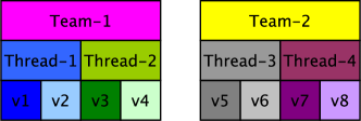
Figure 1: Thread hierarchy used in Figure 2 and Figure 3. Two teams have two threads with two vector lanes each.

Figure 2 and  3 give examples of different partitioning schemes. Figure 1 shows our Kokkos-thread hierarchy used in this example.

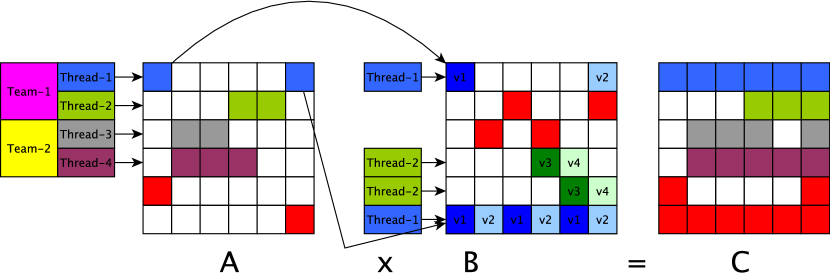
(a) Thread-Sequential: Thread-1 is assigned to a single row of $A$. It sequentially traverses the corresponding rows of $B$, one and six. It exploits vector parallelism for rows of $B$.

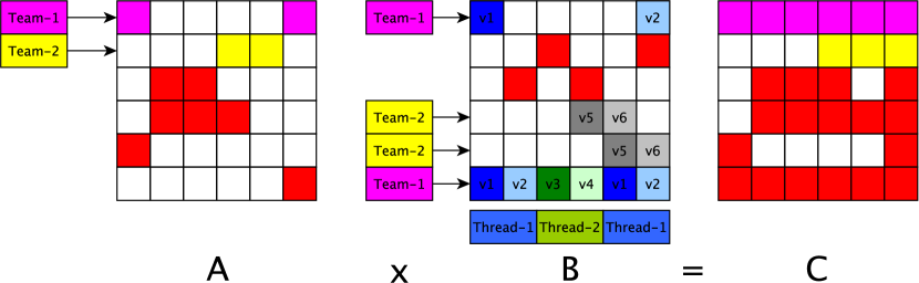
(b) Team-Sequential:Team-1 is assigned to a single row of $A$. It sequentially traverses the corresponding rows of $B$, one and six. It exploits both thread and vector parallelism for rows of $B$.

Figure 2: Partitioning schemes for spgemm using Kokkos-thread hierarchy. Nonzeroes and zeroes are shown in red and white, respectively. Other colors represent the mapping of the data to execution units given in Figure 1.

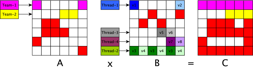
(a) Thread-Parallel: Team-1 is assigned to a single row of $A$. Thread-1 and Thread-2 work on first and sixth rows of $B$ in parallel. They further exploit vector parallelism for rows of $B$.

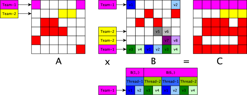
(b) Thread-Flat-Parallel: Team-1 is assigned to single row of $A$. The multiplications are flattened as shown in the bottom, and both thread and vector parallelism are exploited in this single dimension. Thread-1 and thread-2 work on different portions of the sixth row of $B$

Figure 3: Partitioning schemes for spgemm using Kokkos-thread hierarchy.

Thread-Sequential: As shown in Figure 2a, this partitioning scheme assigns a group of rows to different teams, e.g. team-1 gets the first two rows. Each thread within the team works on a different row (Line-3 of Algorithm 3 is executed in parallel by threads). Threads traverse the nonzeroes ($A(i,j)$) of their assigned row $A(i,:)$, and the corresponding rows $B(j,:)$ sequentially (Line-4). The nonzeroes of $B(j,:)$ are traversed, multiplied and inserted into accumulators using vector parallelism (Line-5). A single thread computes the result for a single row of $C$ using vectorlanes. Our previous work, kkmem [13], and AmgX follow this partitioning scheme. Team resources (e.g., shared memory used for $\mathcal{L}_{1}$ accumulators in gpus) are disjointly shared by the threads. This might cause more frequent use of $\mathcal{L}_{2}$ accumulators (located in slower memory space) for larger rows. The partitioning scheme, on the other hand, allows atomic-free accumulations. All computational units work on a single row of $B$ at a time, which guarantees unique value insertions to the accumulators.

Team-Sequential: In Figure 2b, team-1 and team-2 are assigned the first and second row, respectively. Different from Thread-Sequential, a whole team works on a single row of $A$ (Line-3 sequential). Then, the whole team also sequentially traverses the nonzeroes ($A(i,j)$) of $A(i,:)$ (Line-4). Finally, the nonzeroes in row $B(j,:)$ are traversed, multiplied and inserted into accumulators using both thread and vector parallelism (Line-5). This approach can use all of a team’s resources when computing the result of a single row. This allows $\mathcal{L}_{1}$ to be larger, and thus reduces the number of $\mathcal{L}_{2}$ accesses. It also guarantees unique value insertions. However, execution units are likely to be underutilized when the average row size of $B$ is small. Unless we have a very dense multiplication, our preliminary experiments show that this method does not have advantages over other methods. As a result, we do not use this method in our comparisons.

Thread-Parallel: Figure 3a gives an example of this scheme. This scheme assigns a whole team to a single row of $A$ (sequential Line-3). The method parallelizes both of the loops at Line-4 and Line-5. Threads are assigned to different nonzeroes of ($A(i,j)$) of row $A(i,:)$, and the corresponding row $B(j,:)$. Nonzeroes in $B(j,:)$ are traversed, multipled and inserted into accumulators using vector parallelism (Line-5). As in Team-Sequential, more team resources are available for $\mathcal{L}_{1}$. The chance of underutilization is lower than in the previous method, but it can still happen when rows require a very small number of multiplications. In addition, threads may suffer from load imbalance, when rows of $B$ differ in sizes. This scheme does not guarantee unique insertions to accumulators, as different rows of $B$ are handled in parallel. This method is used in Nsparse [24] and Kunchum et al. [19].

Thread-Flat-Parallel: We use a Thread-Flat-Parallel scheme (Figure 3b) to overcome the limitations of the previous methods. This has also been explored in [8] and [19]. In this scheme, a row of $A$ is assigned to a team, but as opposed to the Thread-Parallel scheme, this method flattens the second and third loop (Line-4 and Line-5). The single loop iterates over the total number of multiplications required for the row, which is parallelized using both vector and thread parallelism. Each vector unit calculates the index entries of $A$ and $B$ to work on, and inserts its multiplication result into the accumulators. This achieves a load-balanced distribution of the multiplications to execution units. For example, both $B(1,:)$ and $B(6,:)$ are used for the multiplication of $A(1,:)$ in Figure 3b. Vectorlanes are assigned uniformly to the $8$ multiplications. In this scheme, a row of $B$ can be processed by multiple threads, and a single thread can work accross multiple rows. Regardless of the differing row sizes in $B$, this method achieves perfect load-balancing at the cost of performing index calculations for both $A$ and $B$. The approach also provides larger shared memory for $\mathcal{L}_{1}$ than Thread-Sequential. It may underutilize compute units only when rows require a very small number of total multiplications. Parallel processing of the rows of $B$ does not guarantee unique insertions to accumulators.

In this work, we use the Thread-Sequential and the Thread-Flat-Parallel scheme on gpus. These schemes behave similarly when teams have a single thread, our choice for cpus and knls. However, Thread-Flat-Parallel incurs index calculation overhead, which is not amortized when there is not enough parallelism within a team. Thus, Thread-Sequential is used on cpus and knls.

3.1.2 Accumulators and Memory Pool Data Structures

Our main methods use two-level, sparse hashmap-based accumulators. Accumulators are used to compute the row size of $C$ in the symbolic phase, and the column indices and their values of $C$ in the numeric phase. Once teams/threads are created, they allocate some scratch memory (Line 1) for their private level-1 ($\mathcal{L}_{1}$) accumulator (not to be confused with the L1 cache). This scratch memory maps to the gpu shared memory in gpus and the default memory (i.e., ddr4 or high bandwidth memory) on knls. If the $\mathcal{L}_{1}$ accumulator runs out of space, global memory is allocated (Line 9) in a scalable way using memory pools (explained below) for a row private $\mathcal{L}_{2}$ accumulator. Its size is chosen to guarantee that it can hold all insertions. Upon the completion of a row computation, any allocated $\mathcal{L}_{2}$ accumulator is explicitly released. Scratch spaces used by $\mathcal{L}_{1}$ accumulators are automatically released by Kokkos when the threads retire.

We implemented three different types of accumulators. Two of these are sparse hashmap based accumulators, while the third one is a dense accumulator.

Linked List based HashMap Accumulator (LL): Accumulators are either thread or team private based on the partitioning scheme, so they need to be highly scalable in terms of memory. The hashmap accumulator here extends the hashmap used in [12] for parallel insertions. It consists of $4$ parallel arrays. Figure 4b shows an example of a hashmap that has a capacity of $8$ hash entries and $5$ (key, value) pairs. The hashmap is implemented as a linked list structure. $Ids$ and $Values$ store the (key, value) pairs. $Begins$ holds the beginning indices of the linked lists corresponding to the hash values, and $Nexts$ holds the indices of the next elements within the linked list. For example, the set of keys that have a hash value of $4$ are stored with a linked list. The first index of this linked list is stored at $Begins[4]$. We use this index to retrieve the (key, value) pairs ($Ids[0]$, $Values[0]$). The linked list is traversed using the $Nexts$ array. An index value $-1$ corresponds to the end of the linked list for the hash value. We choose the size of $Begins$ to be a power of $2$, therefore hash values can be calculated using BitwiseAnd, instead of slow modulo ($\%$) operation. Each vector lane calculates the hash values, and traverses the corresponding linked list. If a key already exists in the hashmap, values are accumulated.The implementation assumes that no values with the same keys are inserted concurrently. If the key does not exist in the hashmap, vector lanes reserve the next available slot with an atomic counter, and insert it to the beginning of the linked list (atomic_compare_and_swap) of the corresponding hash. If it runs out out memory, it returns “FULL” and the failed insertions are accumulated in $\mathcal{L}_{2}$. Because of its linked list structure, its performance is not affected by the occupancy of the hashmap. Even when it is full, extra comparisons are performed only for hash collisions. This provides constant complexity not only for $\mathcal{L}_{1}$ but also for $\mathcal{L}_{2}$ insertions, which are performed only when $\mathcal{L}_{1}$ is full. This method assumes that concurrent insertions are duplicate-free and avoids atomic operations for accumulations, which holds for Thread-Sequential and Team-Sequential. When this assumption does not hold (Thread-Parallel and Thread-Flat-Parallel), a more complex implementation with reduced performance is necessary.

Linear Probing HashMap Accumulator (LP): Linear probing is a common technique that is used for hashing in the literature. Nsparse applies this method for spgemm. Figure 4c gives the example of a hashmap using LP. The data structure consists of two parallel arrays ($Ids$, $Values$). Initially each hash entry is set to $-1$ to indicate that it is empty. Given an ($id$, $value$) pair, LP calculates a hash value and attempts to insert the pair into the hash location. If the slot is taken, it performs a linear scan starting at the hash location and inserts it to the first available space. For example, in Figure 4c hash for $28$ is calculated as $4$, but as the slot is taken it is inserted to the next available space. The implementation is straightforward and LP can easily be used with any of the $4$ partitioning schemes. However, as the occupancy of the hashmap becomes close to full, the hash lookups become very expensive. This makes it difficult to use LP in a two-level hashing approach. Each insertion to $\mathcal{L}_{2}$ would first perform a full scan of $\mathcal{L}_{1}$, resulting in a complexity of $O(\|$$\mathcal{L}_{1}$$\|)$. Nsparse uses single-level LP, and when rows do not fit into gpus shared memory, this accumulator is directly allocated in global memory. In order to overcome this, we introduce a max occupancy parameter. If the occupancy of $\mathcal{L}_{1}$ is larger than this cut-off, we do not insert any new $Ids$ to $\mathcal{L}_{1}$ and use $\mathcal{L}_{2}$ for failed insertions. We observe significant slowdowns with LP once occupancy is higher than $50\%$, which is used as a max occupancy ratio.

Dense Accumulators: This approach accumulates rows in their dense format, requiring space $O(k)$ per thread/team. A dense structure allows columns to be accessed simply using their indices. This removes some overheads such as hash calculation and collisions. Its implementation usually requires $2$ parallel arrays. The first is used for floating point values (initialized with $0$s). A second boolean array acts as a marker array to check if a column index was inserted previously. The column array of $C$ is used to hold the indices that are inserted in the dense accumulator (requires an extra array in the symbolic phase). This is a single-level accumulator, and because of its high memory requirements dense accumulators are not suitable for gpus. The approach is used by Patwary et al. [26] with a column-wise partitioning of $B$ to reduce this memory overhead.

Memory Pool: Algorithm 3 requires a portable, thread-scalable memory pool to allocate memory for $\mathcal{L}_{2}$ “sparse” accumulators, in case a row of $C$ cannot fit into the $\mathcal{L}_{1}$ accumulator. The memory pool is allocated and initialized before the kernel call and services requests to allocate and release memory from thousands of threads/teams. As a result, allocate and release have to be thread scalable. Its allocate function returns a chunk of memory to a requestor thread and locks it. This lock is released as soon as the thread releases the chunk back to the pool. The memory pool reserves numChunks memory chunks, where each has a fixed size (chunkSize). chunkSize is chosen based on the “maximum row size in $C$” (maxrs) to guarantee enough space for the work in any row of $C$. maxrs is not known before performing the symbolic phase so it uses an upper bound. The upper bound is the maximum number of multiplies (maxrf) required by any row. That number can be computed by summing the size of all rows of $B$ that contribute to a row. The memory pool has two operational modes: unique and non-unique mapping of chunks to threads (one2one and many2many).

The parameters of the memory pool are architecture specific. numChunks is chosen based on the available concurrency in an architecture. It is an exact match to the number of threads on the knls/cpus. On gpus, we over-estimate the concurrency to efficiently acquire memory. We check the available memory, and reduce numChunks if the memory allocation becomes too expensive on gpus. cpus/knls use one2one and gpus use many2many. The allocate function of the memory pool uses thread indices. These indices assist the look-up for a free chunk. The pool directly returns the chunk with the given thread index when using the one2one mode. This allows cpu/knl threads to reuse local NUMA memory regions. In the many2many mode, the pool starts a scan from the given thread-index until an available chunk is found. If the memory pool does not immediately have a memory chunk available to fulfill a request, the requesting computational unit spins until it successfully receives an allocation.

3.2 Compression

Compression is applied to $B$ in the symbolic phase. This method, based on packing columns of $B$ as bits, can reduce the size of $B$’s graph up to $32\times$ (the number of bits in an integer). The graph structure of $B$ encodes binary relations - existence of a nonzero in $(i,j)$ or not. This can be represented using single bits. We compress the rows of $B$ such that $32$ columns of $B$ are represented using a single integer following the color compression idea in [11]. In this scheme, the traditional column index array in a compressed-row matrix is represented with $2$ arrays of smaller size: “column set” (cs) and “column set index” (csi). Set bits in cs denote existing columns. That is, if the $i^{th}$ bit in cs is $1$, the row has a nonzero entry at the $i^{th}$ column. cs is used to represent more than $32$ columns. Figure 4a shows an example of the compression of a row with $10$ columns. The original symbolic phase would insert all $10$ columns for this row into accumulators. Compression reduces the row size, and only $2$ are inserted into an accumulator with BitwiseOr operation on cs values. It is more successful if the column indices in each row are packed close to each other.

In Algorithm 3, which computational units scan the rows of $A$ and $C$ only once. However, a nonzero value in $B$ is read multiple times, and there are $flops$ accesses to $B$; i.e., $B(i,:)$ is read as many times as the size of $A(:,i)$. Assuming uniform structure for $A$ with $\delta_{A}$ (average degree of $A$) nonzeroes in each column, each row of $B$ is accessed $\delta_{A}$ times. Thus, $f_{m}$ becomes $O(\delta_{A}\times nnz_{B})$, where $nnz_{B}$ is the number of nonzeroes in $B$. If a compression method with linear time complexity ($O(nnz_{B})$), as the one above, reduces the size of $B$ by some ratio $CF$, the amount of work in the symbolic can be reduced by $O(CF\times\delta_{A}\times nnz_{B})$.

Compression reduces the problem size, allows faster row-union operations using BitwiseOr, and makes the symbolic phase more efficient. The reduction in row lengths of $B$ also reduces the calculated maxrf, the upper bound prediction for the required memory of accumulators in the symbolic phase, further improving the robustness and scalability of the method. However, compression is not always successful at reducing the matrix size. For matrices in which column indices are spread, the compression may not reduce the input size, and introduction of the extra values (cs) may slow the symbolic phase down. For this reason, we run compression in two phases. We first calculate the row sizes in the compressed matrix, and calculate the overall $f_{m}$ after the compression. If $f_{m}$ is reduced more than $15\%$, the matrix is compressed and the symbolic phase is executed using this compressed matrix. Otherwise, we do not perform compression and run the symbolic phase using the original matrices. We find this compression method to be very effective in practice; e.g., the $f_{m}$ reduction is less than $15\%$ only for $7$ of $83$ test cases used in this paper. See [28] for the effect of this compression method on solving the triangle counting problem.

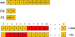
(a) Compression

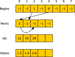
(b) LL

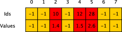
(c) LP

Figure 4: Compression and Hashmap examples

3.3 KokkosKernels SpGEMM Methods

Our previous work [13] proposes the kkmem algorithm. It uses a Thread-Sequential approach with LL accumulators. Its auto parameter detection focuses on the selection of vector-length. This size is fixed for all threads in a parallel kernel. We set it on gpus by rounding $\delta_{B}$ (average degree of $B$) to the closest power of $2$ (bounded by warp size $32$). On knls and cpus, Kokkos sets the length depending on the compiler and underlying architecture specifications. The size of its $\mathcal{L}_{1}$ accumulators depends on the available shared memory on gpus. The size of the $\mathcal{L}_{2}$ accumulator (in the global memory) is chosen as maxrs in the numeric (maxrf in the symbolic). In contrast to gpus, both $\mathcal{L}_{1}$ and $\mathcal{L}_{2}$ accumulators are in the same memory space on knls/cpus. Since there are more resources per thread on the knls/cpus, we make $\mathcal{L}_{1}$ big enough to hold maxrs (or maxrf). This is usually small enough to fit into cache on knls/cpus.

kkmem is designed to be scalable to run on large datasets with large thread counts. It aims to minimize the memory use ($O($maxrs$)$) and to localize memory accesses at the cost of increased hash operations/collisions. In this work, we add kkdense that uses dense accumulators ($O(k)$) and runs only on cpus and knls. It does not have the extra cost of hash operations. However, its memory accesses may not be localized depending on the structure of a problem. When $k$ is small, using sparse accumulators does not have much advantage over dense accumulators (on knls/cpus) as a dense accumulator would also fit into cache. Moreover, some matrix multiplications might result in maxrs to be very close to $k$ (e.g. squaring RMAT matrices results in maxrs to be $95\%$ of $k$). In such cases sparse accumulators allocate as much memory as dense accumulators, while still performing extra hash operations. Sparse accumulators are naturally not expected to perform better than dense accumulators for these cases.

This work proposes a meta algorithm kkspgemm that chooses either of these methods on cpus and knls based on the size of $k$. We observe superior performance of kkdense for $k<250,000$ on knl’s ddr memory. As $k$ gets larger kkmem outperforms kkdense. We introduce a cut-off parameter for $k$ based on this observation. The meta-algorithm runs kkdense for $k<250,000$, and kkmem otherwise. As the columns are compressed in the symbolic phase by a factor of $32$, kkspgemm may run kkdense for the symbolic phase, and kkmem for the numeric phase. A more sophisticated selection of this parameter requires consideration of the underlying architecture. If the architecture has a larger memory bandwidth, it may be more tolerant to larger dense accumulators. For example, using mcdram or cache-mode in knls provides larger memory bandwidth, and kkdense also achieves better performance than kkmem for $k>250,000$. Yet, in the rest of the paper we use $k=250,000$ as cut-off across different architectures, which captures the best methods for most cases.

The parameter selection on gpus is more complicated with additional variables, i.e., shared memory, warp (vector-length) and block sizes. This work introduces kklp, which uses the Thread-Flat-Parallel partitioning with two-level LP accumulators. For problems in which rows require few (on average $<256$) multiplications, our meta algorithm runs kkmem; otherwise it runs kklp. Once the algorithm is chosen, based on the average output row size (ars), we adjust the shared memory size (initially $16$KB per team) to minimize the use of $\mathcal{L}_{2}$ accumulators. For kkmem, if ars does not fit into $\mathcal{L}_{1}$, we reduce the number of threads within teams (by increasing the vector length up to $32$ and reducing threads at the same time) to increase the shared memory per thread, so that most of the entries can fit into $\mathcal{L}_{1}$. For kklp, if initial available shared memory for the team ($16$KB) provides more space than ars, we reduce the team size and its shared memory to be able to run more blocks concurrently on the streaming multiprocessors of gpus. If ars requires larger memory than $16$KB, we increase the shared memory at most to $32$KB (and block size to $512$). As the row sizes are unknown at the beginning of the symbolic phase, it is more challenging to select these parameters then. We estimate ars from $f_{m}$ by assuming every $n$th ($8$th is used for the experiments) multiplication will reduce to the same nonzero.

The experiments run our old method kkmem without this parameter selection to highlight the improvements w.r.t. previous work. Table 1 summarizes the methods used in this paper. Our implementations cannot launch concurrent kernels using cuda-streams as Nsparse does, as Kokkos does not support that yet. Instead, we launch a single kernel using the above parameter selection.

Table 1: The KokkosKernels variants used in this paper.

cpus & knls	kkmem [13]	kkdense: Dense Acc.	kkspgemm: kkmem for $k<250,000$, kkdense otherwise.
gpus	kkmem [13]	kklp: 2-level LP with Thread-Flat-Parallel	kkspgemm: kkmem for average row flops$<256$, kklp otherwise.

4 Experiments

Table 2: The specifications of the architectures used in the experiments. The experiments set OMP_PROC_BIND=spread and OMP_PLACES=threads.

Cluster - cpu/gpu	Bowman - Intel KNL	White (Host) - IBM Power8	White (GPU) - NVIDIA P100-SXM2
Compiler	intel 18.0.128	gnu 5.4.0	gnu 5.4.0, nvcc 8.0.44
Core specs	$68\times 1.40$GHz cores, 4 hyperthreads	$16\times 3.60$ GHz cores, 8 hyperthreads	$1.48$GHz
Memory	$16$ GB MCDRAM $460$ GB/s, $96$ GB DDR4 $102$ GB/s	$512$ GB DDR4, $2$ NUMA	$16$ GB HBM

Performance experiments are performed on three different configurations, representing two of the most commonly HPC leadership class machine hardware designs: Intel XeonPhi and IBM Power with NVIDIA GPUs. The configurations of the nodes are listed in Table 2. Our methods are implemented using the Kokkos library (2.5.00), and will be available in KokkosKernels (2.5.10). Detailed explanation about the raw experiment results and reproducing them can be found at https://github.com/kokkos/kokkos-kernels/wiki/SpGEMM_Benchmarks. Each run reported in this paper is the average of $5$ executions (preceded with $1$ excluded warmup run) with double precision arithmetic and $32$ bit integers. We evaluate $83$ matrix multiplications, $24$ of which are of the form $R\times A\times P$ as found in multigrid, while the rest are of the form $A\times A$ using matrices from the UF sparse suite [9]. The problems are listed in Table 3.Experiments are run for both a NoReuse and a Reuse case. Both the symbolic and the numeric phase are executed for NoReuse. Reuse executes only the numeric phase, and reuses the previous symbolic computations. Unless specifically stated, the results refer to the NoReuse case.

Table 3: The list of the matrices used in the experiments in this paper. CF and CMRF gives the ratio of the reduction in overall number of flops and maximum row flops. Last four columns list the achieved GFLOPs/sec by kkspgemm on $4$ architectures.

ID	Multiplication	$m$	$n$	$k$	$f_{m}$	maxrf	$\|$C$\|$	maxrs	CF	CMRF	Power8	P100	KNL DDR	KNL CACHE
1	amazon0302	262,111	262,111	262,111	6,021,131	25	3,896,236	25	0.71	1.00	1.63	1.64	0.80	0.89
2	belgium_osm	1,441,295	1,441,295	1,441,295	7,017,228	25	5,323,073	18	0.65	0.80	1.36	1.13	0.60	0.66
3	mac_econ_fwd500	206,500	206,500	206,500	7,556,897	229	6,704,899	215	0.57	0.59	2.22	1.49	0.51	0.72
4	mc2depi	525,825	525,825	525,825	8,391,680	16	5,245,952	10	0.76	0.94	2.55	1.51	1.00	1.65
5	delaunay_n18	262,144	262,144	262,144	9,907,810	214	5,430,294	154	0.47	0.62	3.25	2.18	1.07	1.38
6	2cubes_sphere	101,492	101,492	101,492	27,450,606	544	8,974,526	180	0.48	0.63	5.15	5.80	1.45	2.57
7	ca-HepPh	12,008	12,008	12,008	30,793,000	93,923	3,284,660	3,211	0.73	0.03	7.59	1.48	2.36	2.35
8	rgg_n_2_18_s0	262,144	262,144	262,144	39,648,378	716	9,179,295	67	0.81	0.70	5.09	6.82	2.51	3.20
9	hugetrace-00000	4,588,484	4,588,484	4,588,484	41,260,426	9	28,308,760	7	0.74	1.00	1.06	3.16	0.54	0.83
10	web-Stanford	281,903	281,903	281,903	44,110,669	13,682	20,811,442	3,421	1.00	0.64	3.60	2.12	1.69	2.13
11	Stanford	281,903	281,903	281,903	44,110,669	491,041	20,811,442	68,455	0.86	0.03	1.99	0.19	0.44	0.83
12	amazon-2008	735,323	735,323	735,323	46,082,867	100	25,366,745	100	0.38	0.93	3.88	3.65	2.03	2.67
13	web-Google	916,428	916,428	916,428	60,687,836	4,334	29,710,164	2,256	1.00	1.00	2.13	1.81	1.21	1.92
14	webbase-1M	1,000,005	1,000,005	1,000,005	69,524,195	116,179	51,111,996	12,383	0.25	0.27	4.23	1.19	1.54	1.82
15	offshore	259,789	259,789	259,789	71,342,515	562	23,356,245	182	0.61	0.68	5.22	7.29	2.75	3.97
16	conf5_4-8x8-05	49,152	49,152	49,152	74,760,192	1,521	10,911,744	222	0.21	0.26	12.34	10.78	4.42	5.45
17	delaunay_n21	2,097,152	2,097,152	2,097,152	79,241,506	219	43,417,524	157	0.47	0.65	3.55	4.95	1.73	2.48
18	cop20k_A	121,192	121,192	121,192	79,883,385	2,489	18,705,069	495	0.39	0.43	6.90	10.11	2.94	4.40
19	cit-Patents	3,774,768	3,774,768	3,757,431	82,152,992	6,142	68,848,721	3,925	0.99	0.99	0.89	0.90	0.54	1.07
20	filter3D	106,437	106,437	106,437	85,957,185	3,340	20,161,619	550	0.54	0.63	7.61	8.16	3.29	5.11
21	Empire_RAxP	8,800	2,160,000	8,800	91,604,280	11,037	280,800	36	0.59	0.03	5.86	3.02	2.78	3.61
22	Empire_RxAP	8,800	2,160,000	8,800	91,604,280	11,064	280,800	36	0.39	0.03	6.24	5.12	3.17	4.38
23	cnr-2000	325,557	325,557	325,557	96,065,788	34,537	34,174,066	15,723	0.18	0.19	7.32	2.13	3.16	5.12
24	soc-Slashdot0811	77,360	77,360	77,360	111,839,175	134,321	78,851,659	31,750	0.60	0.03	4.58	1.56	1.46	2.46
25	amazon0601	403,394	403,394	403,394	149,306,190	31,313	98,600,816	20,607	0.79	0.40	3.40	1.40	1.20	2.03
26	rma10	46,835	46,835	46,835	156,480,259	12,765	7,900,917	425	0.10	0.10	15.89	16.65	8.25	9.51
27	hugebubbles-00000	18,318,143	18,318,143	18,318,143	164,791,952	9	113,009,849	7	0.74	1.00	1.03	4.02	0.73	1.02
28	hugebubbles-00020	21,198,119	21,198,119	21,198,119	190,713,076	9	132,690,161	7	0.83	1.00	0.57	3.28	0.57	0.82
29	rgg_n_2_20_s0	1,048,576	1,048,576	1,048,576	194,980,566	1,011	41,709,507	75	0.90	0.74	5.28	8.10	3.37	4.24
30	Elasticity_113_RxAP	54,872	4,328,691	54,872	205,253,787	3,993	1,404,928	27	0.47	0.43	5.25	5.75	3.13	4.47
31	Elasticity_113_RAxP	54,872	4,328,691	54,872	205,253,787	3,993	1,404,928	27	0.65	0.43	5.25	3.51	2.75	4.11
32	Stanford_Berkeley	683,446	683,446	683,446	222,116,841	955,984	78,130,972	136,877	0.17	0.03	4.49	0.49	1.40	1.57
33	europe_osm	50,912,018	50,912,018	50,912,018	241,277,568	44	182,570,158	28	0.64	0.80	1.32	2.82	0.87	1.17
34	cant	62,451	62,451	62,451	269,486,473	5,913	17,440,029	375	0.12	0.12	15.82	18.99	9.36	12.89
35	Brick_185_RxAP	238,328	6,331,625	238,328	307,568,462	2,220	6,436,594	78	0.47	0.71	5.37	6.79	3.02	4.21
36	Brick_185_RAxP	238,328	6,331,625	238,328	307,568,462	2,217	6,436,594	78	0.64	0.78	5.25	3.82	3.07	4.16
37	BigStar_4657_RAxP	1,446,620	21,687,649	1,446,620	369,829,182	265	24,552,796	17	0.79	0.80	2.47	4.53	1.36	2.63
38	BigStar_4657_RxAP	1,446,620	21,687,649	1,446,620	369,829,182	265	24,552,796	17	0.63	0.67	2.29	5.64	1.27	2.68
39	shipsec1	140,874	140,874	140,874	450,639,288	6,876	24,086,412	342	0.15	0.17	15.67	21.58	10.63	13.30
40	consph	83,334	83,334	83,334	463,845,030	6,561	26,539,736	375	0.15	0.24	16.10	25.88	11.03	13.72
41	cage14	1,505,785	1,505,785	1,505,785	532,205,737	1,525	236,999,813	646	0.78	0.74	4.76	4.85	2.89	4.11
42	pdb1HYS	36,417	36,417	36,417	555,322,659	32,222	19,594,581	987	0.07	0.04	18.64	24.47	12.69	15.60
43	hood	220,542	220,542	220,542	562,028,138	3,871	34,242,180	231	0.13	0.16	15.28	25.34	9.44	12.45
44	Laplace_284_RxA	2,774,624	22,906,304	22,906,304	582,550,744	350	206,478,136	114	0.72	0.73	2.13	4.58	0.87	2.05
45	Laplace_284_AxP	22,906,304	22,906,304	2,774,624	582,550,744	36	206,478,136	15	0.93	1.00	3.42	6.76	2.40	2.89
46	af_shell1	504,855	504,855	504,855	613,607,875	1,375	47,560,375	105	0.11	0.15	11.53	26.17	8.55	9.78
47	pwtk	217,918	217,918	217,918	626,054,402	8,474	32,772,236	384	0.09	0.10	16.43	33.24	10.79	13.60
48	delaunay_n24	16,777,216	16,777,216	16,777,216	633,914,372	280	347,322,258	218	0.47	0.69	3.57	6.72	2.23	3.11
49	Laplace_284_RxAP	2,774,624	22,906,304	2,774,624	742,456,340	422	86,570,980	49	0.83	0.91	2.34	6.19	1.05	2.11
50	Laplace_284_RAxP	2,774,624	22,906,304	2,774,624	742,456,340	404	86,570,980	49	0.93	0.97	2.84	4.76	1.02	2.11
51	Brick_185_RxA	238,328	6,331,625	6,331,625	776,170,999	5,751	78,955,509	509	0.35	0.35	6.42	7.98	4.43	6.10
52	Brick_185_AxP	6,331,625	6,331,625	238,328	776,170,999	215	78,955,509	27	0.61	0.83	6.94	11.70	4.69	5.66
53	nlpkkt80	1,062,400	1,062,400	1,062,400	790,384,704	784	154,663,144	152	0.38	0.48	7.64	12.43	6.10	7.17
54	BigStar_4657_AxP	21,687,649	21,687,649	1,446,620	845,292,479	42	131,484,200	9	0.78	0.98	4.14	9.60	2.98	3.57
55	BigStar_4657_RxA	1,446,620	21,687,649	21,687,649	845,292,479	585	131,484,200	91	0.40	0.42	3.82	7.71	2.15	4.08
56	eu-2005	862,664	862,664	862,664	849,268,919	153,454	284,177,131	16,051	0.28	0.10	5.48	5.44	2.06	2.78
57	NALU_R3_RxAP	552,583	17,598,889	552,583	1,254,217,679	3,357	31,098,707	59	0.46	0.68	5.27	8.91	3.94	5.16
58	NALU_R3_RAxP	552,583	17,598,889	552,583	1,254,217,679	3,219	31,098,707	59	0.67	0.77	4.75	4.78	3.40	4.56
59	Empire_RxA	8,800	2,160,000	2,160,000	1,286,511,829	155,460	25,410,400	3,010	0.15	0.17	8.16	8.66	5.55	6.56
60	Empire_AxP	2,160,000	2,160,000	8,800	1,286,511,829	999	25,410,400	27	0.55	0.28	8.36	8.85	6.46	7.42
61	Fault_639	638,802	638,802	638,802	1,298,780,298	15,813	126,633,024	897	0.19	0.16	11.06	17.47	8.63	10.46
62	channel-500x100x100-b050	4,802,000	4,802,000	4,802,000	1,522,677,096	324	436,529,632	93	0.52	0.74	6.31	11.41	4.77	6.00
63	wb-edu	9,845,725	9,845,725	9,845,725	1,559,579,990	281,616	630,077,764	14,427	0.21	0.12	4.25	7.07	1.31	1.40
64	Elasticity_113_AxP	4,328,691	4,328,691	54,872	1,572,091,911	375	53,338,743	27	0.61	0.74	8.31	12.86	6.39	7.55
65	Elasticity_113_RxA	54,872	4,328,691	4,328,691	1,572,091,911	30,375	53,338,743	1,029	0.14	0.14	9.43	12.64	7.23	8.93
66	in-2004	1,382,908	1,382,908	1,382,908	1,708,503,481	240,257	213,255,458	9,997	0.08	0.09	4.59	5.80	1.85	2.07
67	af_shell10	1,508,065	1,508,065	1,508,065	1,840,916,875	1,225	142,742,975	95	0.11	0.16	12.10	27.42	9.99	11.49
68	cage15	5,154,859	5,154,859	5,154,859	1,885,387,372	1,904	929,023,247	859	0.83	0.79	4.57	5.72	2.78	4.33
69	dielFilterV2real	1,157,456	1,157,456	1,157,456	2,337,362,192	5,464	325,027,200	668	0.30	0.36	8.76	13.36	7.12	8.64
70	wikipedia-20051105	1,634,989	1,634,989	1,634,989	2,373,873,670	274,992	1,725,264,272	134,091	0.82	0.19	3.33		0.99	1.16
71	ldoor	952,203	952,203	952,203	2,408,881,377	4,165	145,422,935	259	0.12	0.16	12.22	24.74	10.70	12.08
72	NALU_R3_RxA	552,583	17,598,889	17,598,889	2,456,399,623	6,777	243,321,996	613	0.28	0.32	6.37	8.20	4.44	6.49
73	NALU_R3_AxP	17,598,889	17,598,889	552,583	2,456,399,623	183	243,321,996	22	0.67	0.90	5.38	11.50	4.37	4.93
74	Serena	1,391,349	1,391,349	1,391,349	3,111,966,351	11,556	315,805,689	1,236	0.18	0.18	11.33	17.13	10.07	11.26
75	coPapersDBLP	540,486	540,486	540,486	4,091,407,036	737,309	480,122,442	35,874	0.17	0.03	10.18	7.89	5.20	7.81
76	flickr	820,878	820,878	820,878	4,318,945,024	2,907,529	1,112,536,788	202,990	0.57	0.03	4.45	1.45	1.28	2.17
77	RM07R	381,689	381,689	381,689	5,272,142,064	60,375	193,345,783	1,475	0.15	0.15	11.81	20.33	10.08	12.15
78	Bump_2911_dig	2,911,419	2,911,419	2,911,419	5,745,156,927	9,370	560,173,611	738	0.17	0.17	11.29	19.54	10.49	11.39
79	kron_g500-logn16	65,536	65,536	65,536	6,768,428,563	4,368,565	972,785,311	54,856	0.50	0.03	8.44	2.49	2.66	3.63
80	coPapersCiteseer	434,102	434,102	434,102	6,822,448,658	786,040	264,584,716	12,882	0.10	0.03	8.81	19.43	5.59	7.50
81	audikw_1	943,695	943,695	943,695	8,089,734,897	32,985	662,878,935	1,689	0.14	0.14	11.71	19.70	9.92	11.80
82	dielFilterV3real	1,102,824	1,102,824	1,102,824	8,705,461,058	26,163	688,649,400	1,671	0.23	0.26	10.47	17.04	8.60	10.83
83	HV15R	2,017,169	2,017,169	2,017,169	42,201,218,799	132,295	1,768,066,720	1,900	0.13	0.14	13.00		10.25	8.22
								GEOMEAN:	0.38	0.30	5.23	5.98	2.86	3.90

4.1 Experiments on Power8 cpus

We compare our methods (kkspgemm, kkmem, kkdense), against ViennaCL (OpenMP) on Power8 cpus. Figure 5 gives strong scaling GFLOPS/sec for the four methods on different multiplications with different characteristics.

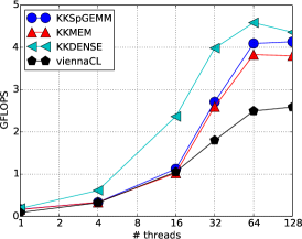
(a) BigStar $A\times P$ $k=1.5M$

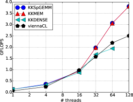
(b) BigStar $R\times A$ $k=21.5M$

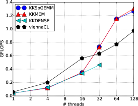
(c) europe $k=50.9M$

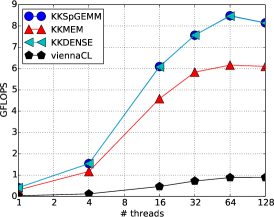
(d) kron16 $k=65K$

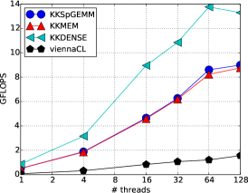
(e) coPap.Cite. $k=434K$

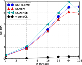
(f) flickr $k=820K$

Figure 5: Strong scaling GFLOPS/sec on Power8 cpus.

The first two multiplications (a and b) are from a multigrid problem. As $k$ gets larger, kkdense suffers from low spatial locality, and it is outperformed by kkmem. kkdense’s memory allocation for its accumulators fails for some cases. Although, they should fit into memory, we suspect that allocation of such large chunks is causing these failures. kkdense achieves better performance for matrices with smaller $k$. Among them, kron not only has the smallest $k$, but also has a maxrs that is $83\%$ of $k$. The sparse accumulators use a similar amount of memory as kkdense, but still acrue the overhead for hash operations. Our meta method chooses kkdense for kron’s numeric and the symbolic phase. It executes kkdense only for the symbolic phase of BigStar $A\times P$, coPapersCiteseer, and flickr, as the compression reduces their $k$ by $32\times$. kkdense achieves better performance than kkspgemm in $3$ instances. These suggest that the simple architecture agnostic heuristic for choosing the optimal algorithm, is leaving room for improvement. The current heuristic is erring on the side of reduced memory consumption, which in real applications may be desirable.

Figure 6a lists the performance profiles of the algorithms on Power8. For a given $x$, the $y$ value indicates the number of problem cases, for which a method is less than $x$ times slower than the best result achieved with any method for each individual problem. The max value of $y$ at $x=1$ is the number of problem cases for which a method achieved the best performance. The $x$ value for which $y=83$ is the largest slowdown a method showed over any problem, compared with the best observed performance for that problem over all methods. As seen in the figure, for about $50$ problems kkspgemm achieves the best performance (or at most $0.5\%$ slower than the best KK variant). The performance of viennaCL is mostly lower than achieved by KK variants. While our methods do not make any assumption on whether the input matrices have sorted columns, all test problems have sorted columns to be able to run the different methods throughout our experiments. For example, viennaCL requires sorted inputs, and returns sorted output. If the calling application does not store sorted matrices, pre-processing is required to use viennaCL. Similarly, if the result of spgemm must be sorted, post-processing is required for our methods. For iterative multiplications in multigrid, the output of a multiplication ($AP=A\times P$) becomes the input of the next one ($R\times AP$). As long as methods make consistent assumptions for their input and outputs, this pre-/post-processing can be skipped.

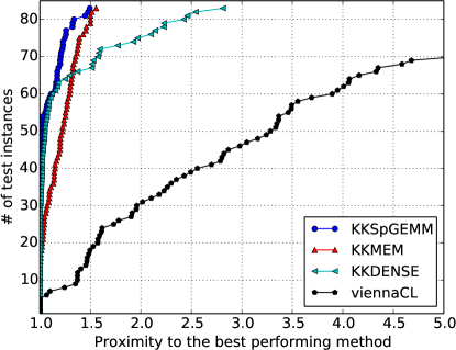
(a) Power8 NoReuse

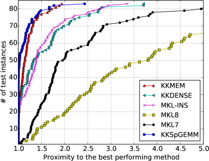
(b) knl ddr NoReuse

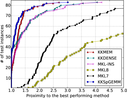
(c) knl CM NoReuse

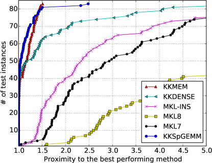
(d) knl CM Reuse

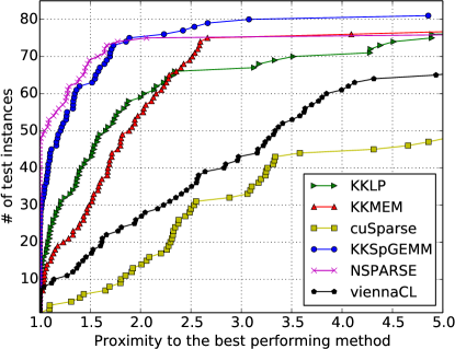
(e) P100 NoReuse

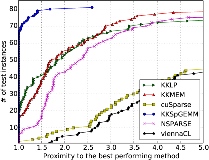
(f) P100 Reuse

Figure 6: Performance profiles on Power8, knl, and P100 gpus. Experiments on gpus include $81$ multiplications, as result $C$ does not fit into memory.

4.2 Experiments on knls

The experiments on knls compare our methods against two methods provided by the Intel Math Kernel Library (mkl) using two memory modes. The first uses the high bandwidth memory (mcdram) of knls as a cache (CM), while the second runs in flat memory mode using only ddr. mkl_sparse_spmm in mkl’s inspector-executor is referred to as mkl-ins, and the mkl_dcsrmultcsr is referred to as mkl7 and mkl8. mkl_dcsrmultcsr requires sorted inputs, without necessarily returning sorted outputs. Output sorting may be skipped for $A\times A$ (e.g., graph analytic problems); however, it becomes an issue for multigrid. The results report both mkl7 (without output sorting) and mkl8 (with output sorting). mkl’s expected performance is the performance of mkl7 for $A\times A$ and mkl8 for multigrid multiplications.

(a) coPapersCiteseer ddr

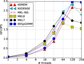
(b) BigStar $A\times P$ ddr

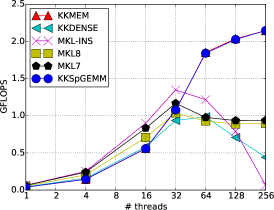
(c) BigStar $R\times A$ ddr

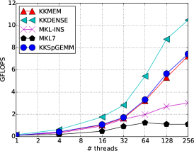
(d) coPapersCiteseer CM

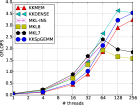
(e) BigStar $A\times P$ CM

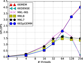
(f) BigStar $R\times A$ CM

Figure 7: Strong scaling GLOPS/sec on knls. Top and bottom figures are for flat ddr and CM, respectively. mkl8 does not complete in the given allocation time for coPapersCiteseer.

Figure 7 shows strong scaling GFLOPS/sec of six methods on three multiplications for CM and ddr with number of threads. Since we use maximally 64 cores, 128 and 256 threads use 2 or 4 hyperthreads per cores respectively. Memory accesses on ddr are relatively more expensive than CM; therefore methods using sparse accumulators tend to achieve better scaling and performance. kkdense is usually outperformed by kkmem on ddr except on coPapersCiteseer. CM provides more bandwidth which boosts the performance of all methods. When the bandwidth is not saturated, methods have similar performances on ddr and mcdram, which is observed up to $32$ threads. CM improves the performance of methods which stress memory accesses more, e.g. kkdense. In general, methods favoring memory accesses over hash computations are more likely to benefit from CM than those that already have localized memory accesses. kkspgemm mostly achieves the best performance except for coPapersCiteseer. The higher memory bandwidth of CM allows the use of dense accumulators for larger $k$. $k$ is still too large to benefit from CM for $R\times A$. mkl methods achieve better performance on lower thread counts, but they do not scale with hyperthreads. mkl-ins has the best performance among mkl methods.

It is worthwhile to note that these thread scaling experiments conflate two performance critical issues: thread-scalability of an algorithm, and the amount of memory bandwidth and load/store slots available to each thread. The latter issue would still afflict performance if these methods are used as part of an MPI application, where for example 8 MPI ranks each use 32 threads on KNL. In such a usecase we would expect the relative performance of the methods to be closer to the $256$ thread case than the $32$ thread case in our experiments.

Figure 6 shows performance profiles for NoReuse for ddr, and both NoReuse and Reuse for CM. The experiments on ddr demonstrate the strength of a thread-scalable kkmem algorithm. It outperforms kkdense for larger datasets. Overall, kkspgemm obtains the best performance, taking advantage of kkmem and kkdense for large and small datasets, respectively. kkdense significantly improves its performance on CM w.r.t. ddr. Among mkl methods, mkl-ins achieves the best performance. However, it is a 1-phase method. It cannot exploit structural reuse, and its performance drops for the Reuse case.

4.3 Experiments on GPUs

We evaluate the performance of our methods against Nsparse, cuSPARSE and ViennaCL (1.7.1) on P100 gpus. Figure 6e shows the performance profile on P100 GPUs for NoReuse. Among these methods, kkspgemm and cuSPARSE run for all $81$ instances. kkmem, Nsparse and viennaCL fail for $2$, $4$ and $9$ matrices. cuSPARSE and viennaCL are mostly outperformed by the other methods. These are followed by our previous method kkmem, and our LP based method kklp. kkspgemm takes advantage of kklp, and significantly improves our previous method kkmem with a better parameter setting. As a result, kkspgemm and Nsparse are the most competitive methods. Nsparse, taking advantage of cuda-streams, achieves slightly better performance than kkspgemm. Although the lack of cuda-streams is a limitation for kkspgemm, with a better selection of the parameters it obtains the best performance for $28$ test problems.

Most of the significant performance differences between Nsparse and kkspgemm occur for smaller multiplications that take between $1$ to $10$ milliseconds. Nsparse has the best performance on $18$ out of $20$ multiplications with the smallest number of total $f_{m}$. As the multiplications get larger, the performance of kkspgemm is on average $3-4\%$ better than Nsparse (excluding the smallest $20$ test problems). kkspgemm is also able to perform $4$ test multiplications for which Nsparse runs out of memory (kron16, coPaparciteseer, flickr, coPapersDBLP). The performance comparison of kkspgemm against Nsparse for multiplications sorted based on $f_{m}$ required is shown in Figure 8. This figure reports the geometric mean of the kkspgemm speedups w.r.t. Nsparse. For the smallest $10$ and $20$ multiplications, Nsparse is about $47\%$ and $17\%$ faster than kkspgemm. kkspgemm, on average, has more consistent and faster runtimes for the larger inputs. kkspgemm is designed for scalability, and it introduces various overheads to achieve this scalability (e.g., compression). When the inputs are small, the overhead introduced is not amortized, as the multiplication time is very small even without compression. This makes kkspgemm slower on small matrices, but at the same time it makes kkspgemm more robust and scalable allowing it to run much larger problems. On the other hand, Nsparse returns sorted output rows, which is not the case for kkspgemm. The choice of the better method depends on the application area. If the application requires sorted outputs or the problem size is small, Nsparse is likely to achieve better performance. For the problems with large memory requirements, kkspgemm is the better choice. Lastly, Figure 6f gives the performance profile for the Reuse case. Although Nsparse also runs in two-phases, its current user interface does not allow reuse of the symbolic computations.

The effect of the compression: Compression is critical to reduce the time and the memory requirements of the symbolic phase. It helps to reduce both the number of hash insertions as well as the estimated max row size. Table-1 and 2 (supplementary materials) lists the original $f_{m}$ and maxrf. CF and CMRF give the reduction ratios with compression on $f_{m}$ and maxrf (e.g., $0.85$ means $15\%$ reduction), respectively. On average, $f_{m}$ and maxrf are reduced by $62\%$ and $70\%$. Compression reduces the memory requirements (maxrf) in most cases up to $97\%$. It usually reduces the runtime of the symbolic phase. When the reduction on $f_{m}$ is low (e.g., CF $>0.85$), it might not amortize compression cost. We skip the second-phase of the compression in such cases; however, we still introduce overheads for CF calculations. CF is greater than $0.85$ for only $7$ multiplications, for which the symbolic phase is run without compressed values.

Figure 8: Speedup of kkspgemm w.r.t. NSparse for matrices that are grouped w.r.t. $f_{m}$. These groups can be found using indices in Table 3.

5 Conclusion

We described thread-scalable spgemm kernels for highly threaded architectures. Using the portability provided by Kokkos, we describe algorithms that are portable to gpus and cpus. The performance of the methods is demonstrated on Power8 cpus, knls, and P100 gpus, in which our implementations achieve at least as good performance as the native methods. On cpus and knls, we show that sparse accumulators are preferrable when memory accesses are the performance bottleneck. As memory systems provide more bandwidth (as in mcdram) and $k$ is small, methods with dense accumulators outperform those with sparse accumulators. Although our methods cannot exploit some of the architecture specific details of gpus, e.g., cuda-streams, because of current Kokkos limitations, with a better way of parameter selection we achieve as good performance as highly optimized libraries. The experiments also show that our methods using memory pool and compression techniques are robust and can perform multiplications with high memory demands. Our experiments also highlight the importance of designing methods for application use cases such as symbolic “reuse” with significantly better performance than past methods.

Acknowledgements: We thank Karen Devine for helpful discussions, and the test bed program at Sandia National Laboratories for supplying the hardware used in this paper. Sandia National Laboratories is a multimission laboratory managed and operated by National Technology and Engineering Solutions of Sandia, LLC., a wholly owned subsidiary of Honeywell International, Inc., for the U.S. Department of Energy’s National Nuclear Security Administration under contract DE-NA-0003525.s

References

- [1] The Trilinos project.
- [2] Kadir Akbudak and Cevdet Aykanat. Simultaneous input and output matrix partitioning for outer-product–parallel sparse matrix-matrix multiplication. SIAM Journal on Scientific Computing, 36(5):C568–C590, 2014.
- [3] Kadir Akbudak and Cevdet Aykanat. Exploiting locality in sparse matrix-matrix multiplication on many-core architectures. IEEE Transactions on Parallel and Distributed Systems, 2017.
- [4] Ariful Azad, Grey Ballard, Aydin Buluc, James Demmel, Laura Grigori, Oded Schwartz, Sivan Toledo, and Samuel Williams. Exploiting multiple levels of parallelism in sparse matrix-matrix multiplication. arXiv preprint arXiv:1510.00844.
- [5] Grey Ballard, Alex Druinsky, Nicholas Knight, and Oded Schwartz. Hypergraph partitioning for sparse matrix-matrix multiplication. arXiv preprint arXiv:1603.05627, 2016.
- [6] Aydın Buluç and John R Gilbert. The Combinatorial BLAS: Design, implementation, and applications. International Journal of High Performance Computing Applications, 2011.
- [7] Edith Cohen. Structure prediction and computation of sparse matrix products. Journal of Combinatorial Optimization, 2(4):307–332, 1998.
- [8] Steven Dalton, Luke Olson, and Nathan Bell. Optimizing sparse matrix-—matrix multiplication for the GPU. ACM Transactions on Mathematical Software (TOMS), 41(4):25, 2015.
- [9] Timothy A Davis and Yifan Hu. The University of Florida sparse matrix collection. ACM Transactions on Mathematical Software (TOMS), 38(1):1, 2011.
- [10] Julien Demouth. Sparse matrix-matrix multiplication on the gpu. In Proceedings of the GPU Technology Conference, 2012.
- [11] M. Deveci, E. G. Boman, K. D. Devine, and S. Rajamanickam. Parallel graph coloring for manycore architectures. In 2016 IEEE International Parallel and Distributed Processing Symposium (IPDPS), pages 892–901, May 2016.
- [12] Mehmet Deveci, Kamer Kaya, and Umit V Catalyurek. Hypergraph sparsification and its application to partitioning. In Parallel Processing (ICPP), 2013 42nd International Conference on, pages 200–209. IEEE, 2013.
- [13] Mehmet Deveci, Christian Trott, and Sivasankaran Rajamanickam. Performance-portable sparse matrix-matrix multiplication for many-core architectures. In Parallel and Distributed Processing Symposium Workshops (IPDPSW), 2017 IEEE International, pages 693–702. IEEE, 2017.
- [14] Timothy Dysart, Peter Kogge, Martin Deneroff, Eric Bovell, Preston Briggs, Jay Brockman, Kenneth Jacobsen, Yujen Juan, Shannon Kuntz, Richard Lethin, et al. Highly scalable near memory processing with migrating threads on the emu system architecture. In Irregular Applications: Architecture and Algorithms (IA3), Workshop on, pages 2–9. IEEE, 2016.
- [15] H Carter Edwards, Christian R Trott, and Daniel Sunderland. Kokkos: Enabling manycore performance portability through polymorphic memory access patterns. J Parallel Distrib Comp, 74(12):3202–3216, 2014.
- [16] Felix Gremse, Andreas Hofter, Lars Ole Schwen, Fabian Kiessling, and Uwe Naumann. GPU-accelerated sparse matrix-matrix multiplication by iterative row merging. SIAM Journal on Scientific Computing, 37(1):C54–C71, 2015.
- [17] Fred G Gustavson. Two fast algorithms for sparse matrices: Multiplication and permuted transposition. ACM Transactions on Mathematical Software (TOMS), 4(3):250–269, 1978.
- [18] Intel. Intel math kernel library, 2007.
- [19] Rakshith Kunchum, Ankur Chaudhry, Aravind Sukumaran-Rajam, Qingpeng Niu, Israt Nisa, and P Sadayappan. On improving performance of sparse matrix-matrix multiplication on gpus. In Proceedings of the International Conference on Supercomputing, page 14. ACM, 2017.
- [20] Sureyya Emre Kurt, Vineeth Thumma, Changwan Hong, Aravind Sukumaran-Rajam, and P Sadayappan. Characterization of data movement requirements for sparse matrix computations on gpus. In High Performance Computing (HiPC), 2017 24th International Conference on. IEEE, 2017.
- [21] Paul Lin, Matthew Bettencourt, Stefan Domino, Travis Fisher, Mark Hoemmen, Jonathan Hu, Eric Phipps, Andrey Prokopenko, Sivasankaran Rajamanickam, Christopher Siefert, et al. Towards extreme-scale simulations for low mach fluids with second-generation trilinos. Parallel Processing Letters, 24(04):1442005, 2014.
- [22] Weifeng Liu and Brian Vinter. An efficient gpu general sparse matrix-matrix multiplication for irregular data. In Parallel and Distributed Processing Symposium, 2014 IEEE 28th International, pages 370–381. IEEE, 2014.
- [23] Michael McCourt, Barry Smith, and Hong Zhang. Efficient sparse matrix-matrix products using colorings. SIAM Journal on Matrix Analysis and Applications, 2013.
- [24] Yusuke Nagasaka, Akira Nukada, and Satoshi Matsuoka. High-performance and memory-saving sparse general matrix-matrix multiplication for nvidia pascal gpu. In Parallel Processing (ICPP), 2017 46th International Conference on, pages 101–110. IEEE, 2017.
- [25] M Naumov, LS Chien, P Vandermersch, and U Kapasi. Cusparse library. In GPU Technology Conference, 2010.
- [26] Md Mostofa Ali Patwary, Nadathur Rajagopalan Satish, Narayanan Sundaram, Jongsoo Park, Michael J Anderson, Satya Gautam Vadlamudi, Dipankar Das, Sergey G Pudov, Vadim O Pirogov, and Pradeep Dubey. Parallel efficient sparse matrix-matrix multiplication on multicore platforms. In High Performance Computing, pages 48–57. Springer, 2015.
- [27] K. Rupp, F. Rudolf, and J. Weinbub. ViennaCL - A High Level Linear Algebra Library for GPUs and Multi-Core CPUs. In Intl. Workshop on GPUs and Scientific Applications, pages 51–56, 2010.
- [28] Michael M Wolf, Mehmet Deveci, Jonathan W Berry, Simon D Hammond, and Sivasankaran Rajamanickam. Fast linear algebra-based triangle counting with kokkoskernels. In High Performance Extreme Computing Conference (HPEC), 2017 IEEE, pages 1–7. IEEE, 2017.