11email: robertovio@tin.it, 22institutetext: ESO, Karl Schwarzschild strasse 2, 85748 Garching, Germany
22email: pandrean@eso.org
Matched filter in low-number count Poisson noise regime:
an efficient and effective implementation
The matched filter (MF) is widely used to detect signals hidden within the noise. If the noise is Gaussian, its performances are well-known and describable in an elegant analytical form. The treatment of non-Gaussian noises is often cumbersome as in most cases there is no analytical framework. This is true also for Poisson noise which, especially in the low-number count regime, presents the additional difficulty to be discrete. For this reason in the past methods have been proposed based on heuristic or semi-heuristic arguments. Recently, an analytical form of the MF has been introduced but the computation of the probability of false detection or false alarm () is based on numerical simulations. To overcome this inefficient and time consuming approach we propose here an effective method to compute the based on the saddle point approximation (SA). We provide the theoretical framework and support our findings by means of numerical simulations. We discuss also the limitations of the MF in practical applications.
Key Words.:
Methods: data analysis – Methods: statistical1 Introduction
Detecting signals embedded in noise is a challenge in many research and engineering areas. In the common case of Gaussian noise the standard tool is the matched filter (MF) (Tuzlukov 2001; Minkof 2002; Osche 2002; Briggs 2004; Levy 2008; Yao et al. 2013). According to the Neyman-Pearson theorem, the MF provides the greatest probability of true detection under the condition of a constant probability of false detection (e.g. Kay 1998). In non-Gaussian cases it is difficult to derive an MF and even if available it is more cumbersome to use. In particular, it is complex to compute the probability of false detection or false alarm (PFA). In astronomy this situation occurs, for example, in the search for high-energy point sources in the presence of Poisson (i.e. non-additive) noise and where signal and noise together consist of only a few counts per pixel. For this reason, in the past alternative procedures based on heuristic or semi-heuristic arguments have been preferred (Stewart 2006, and reference therein). In a recent work Ofek & Zackay (2017) provide an analytical form of the MF with the PFA computed from numerical simulations. This approach lacks flexibility and is time-consuming. In the present paper we propose a method to compute the PFA based on the saddle-point approximation (SA) which is fast, flexible and provides accurate results.
In Section 2 the problem of the detection of a signal in Poisson noise is formalized whereas the SA method is described in Sect. 3 and its application illustrated in Sect. 4. The results of a few numerical experiments are given in Sects. 5-6 and the limitations of the MF in practical situations are discussed in Sect. 7. Finally, the conclusions are given in Sect. 8.
2 The mathematics of the problem
In this section we describe the basic properties of the MF in the case of Poisson noise. To allow a better understanding we develop the main arguments in one dimension. The extension to higher dimension cases is straightforward and can be done substituting the coordinate system with a multi-dimensional one 111In the case of a two-dimensional map , a one-dimensional signal is obtained through , with the operator that transforms a matrix into a column array by stacking its columns one underneath the other..
To illustrate the procedure of detection of a deterministic and discrete signal of known structure , with length , and the symbol T denoting a vector or matrix transpose, we assume the following:
-
•
The searched signal takes the form with a positive scalar quantity (amplitude) and typically a smooth function often somehow normalized (e.g., );
-
•
The signal is contaminated by a Poisson noise, i.e. the observed signal is given by . Here, , the scalar represents the intensity parameter of the noise background and denotes a Poisson random vector with independent entries and expected value (i.e. mean) . Although not necessary in what follows, this implies that is constant across .
Under these conditions, the detection problem consists of deciding whether , i.e. it is pure noise (hypothesis ), or it does contain a contribution from a signal (hypothesis ). In this way, it is equivalent to a decision problem between the two hypotheses
| (1) |
Under the probability density function (PDF) of is given by whereas under by . Deciding between these two alternatives requires fixing the detection criterion. A common and effective criterion consists in maximizing the probability of detection () under the constraint that the (i.e., the probability of a false detection) does not exceed a fixed value . The Neyman-Pearson theorem (e.g., see Kay 1998) allows designing a decision process that pursues this aim: to maximize for a given , choose if the likelihood ratio
| (2) |
where the threshold is found from
| (3) |
In a recent work Ofek & Zackay (2017) show that criteria (2) and (3) lead to the test
| (4) |
where
| (5) |
In practice, the test consists of filtering the signal with (i.e. the matched filter) and checking if the statistic exceeds the threshold . From Eq. (5) it appears that the form of depends on the signal . The issue here is that in many practical applications (e.g. detection of point sources in sky maps) only the template of the signal is known but not its amplitude . The consequence of using the MF with an incorrect amplitude is to reduce, for a fixed value of the , the , i.e. to make the MF less efficient. Ofek & Zackay (2017) have shown that the results provided by the MF are not very sensitive to the precise value of (see also below). This is not surprising given the logarithmic dependence of on . However, even for a specific value of , the PDF of under the hypothesis is not available in analytical form. The reason is that, although is given by a linear composition of Poisson random variables, its PDF is not Poissonian. This does not allow fixing the threshold corresponding to a prefixed value of the . Ofek & Zackay (2017) bypass this problem using numerical simulations. Such method, however, is not flexible and is time-consuming.
An alternative to numerical simulations is approximating the unknown PDF of by another PDF. For example, in the situations of high-number count noise regimes, the Gaussian PDF would be a good choice. The same does not hold in low-number count regimes. In this case the SA represents an effective solution.
3 Saddlepoint approximation basics
The SA is a powerful tool able to provide accurate expressions of the PDFs and the corresponding cumulative distribution functions (CDF). Its derivation is rather technical. For this reason, we provide here only a basic introduction useful for practical applications. A simple and informal derivation is outlined in appendix A, whereas a rigorous derivation is given in Butler (2007).
The SA to the PDF of a continuous random variable is given by
| (6) |
where is the cumulant generating function (CGF) of ,
| (7) |
and the corresponding moment generating function (MGF) (see appendix B). Moreover, is the unique solution to the equation
| (8) |
with denoting the th derivative with respect to . will not, in general, integrate to one, although it will usually not be far off. Therefore, it has to be numerically normalized.
The SA results are particularly useful to approximate PDFs not obtainable in analytical form for which the corresponding CGF is available. This situation is typical of a random variable given by the sum of a set of independent random variables , . Indeed, except special cases (e.g., Gaussian), also when the random variables share the same PDF, it is not possible to obtain in closed form. As explained in appendix B, the CGF of a sum of independent random variables is given by the sum of the respective CGFs. Hence, if the CGFs of the random variables are available, the SA can be applied.
Once that is available, the correspoding CDF can be obtained via numerical integration. However, a simple expression, able to provide excellent results, has been proposed by Lugannani & Rice (1980)
| (9) |
Here, and represent the standard Gaussian PDF and CDF, respectively, whereas and are given by
| (10) |
with providing the sign of , and
| (11) |
The only difficulty in using concerns its evaluation when is close to the expected value of . In this case the computation of is tricky since and then the solution of Eq. (8) becomes . As a consequence, it happens that and accordingly, since from Eq. (10), the first equation in the system (9) becomes useless. This is the reason for the second equation in the system (10). For practical use, however, it is numerically more advantageous to use a linear interpolation based on the SA to , where is chosen small enough to ensure high accuracy, but large enough to ensure numerical stability.
In the case is a discrete random variable, the same equations hold with substituted by , which takes values in the set of the integer numbers, and keeping in mind that provides the probability that . Although the expressions (6) and (9) are computable for any value of whether real or integer-valued, and are meaningful approximations of and only for integer-valued arguments.
4 Signal detection in the Poisson noise regime
The SA to the PDF and the CDF of in the Poisson case can be easily computed. Indeed, under the hypothesis , is given by a linear combination (i.e. a sum) of Poisson random variables with common parameter ,
| (12) |
Hence, its CGF is given by
| (13) | ||||
| (14) |
with . It is elementary to see that is given by
| (15) |
In order to be used in Eqs. (6) and (9), these functions have to be computed for . This step requires the numerical solution of Eq. (8) that, however, does not present particular difficulties given that, as explained in appendix A, is an increasing function for .
It is important to stress that, since Eq. (8) cannot be solved when , is defined only for . But it is easy to see that for it is . This last one is an exact result not only an approximation.
When using the SA in the present context, it is necessary to consider that the PDF of is of discrete type but it is not defined on a lattice (i.e. does not take values on a regular grid of numbers). The point is that the arguments presented above hold only for integer values of or, with minor modifications, when takes values on a regular grid of numbers. However, except for extremely small values of , this PDF can be considered “almost continuous”. Indeed, in the case of two-dimensional maps, from combinatorial arguments it can be realized that, already with values of as small as and given by a circular Gaussian with standard deviation of only pixels, the number of different values that can take is of the order of several thousands. In any case, there is considerable empirical evidence that the SA is useful and maintains most of its accuracy even with discrete PDFs not defined on a lattice (cf. pag. 27 in Butler 2007). The numerical simulations presented below confirm this result.
5 Numerical experiments
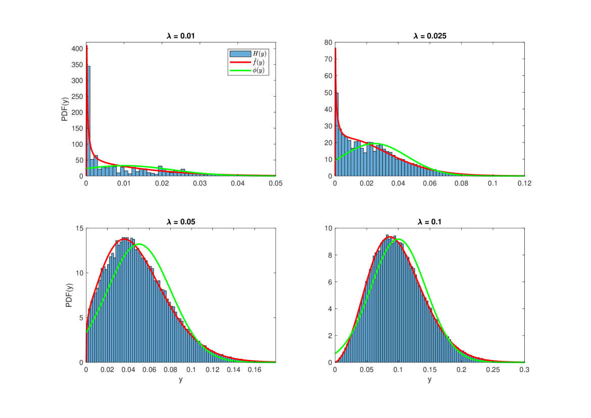
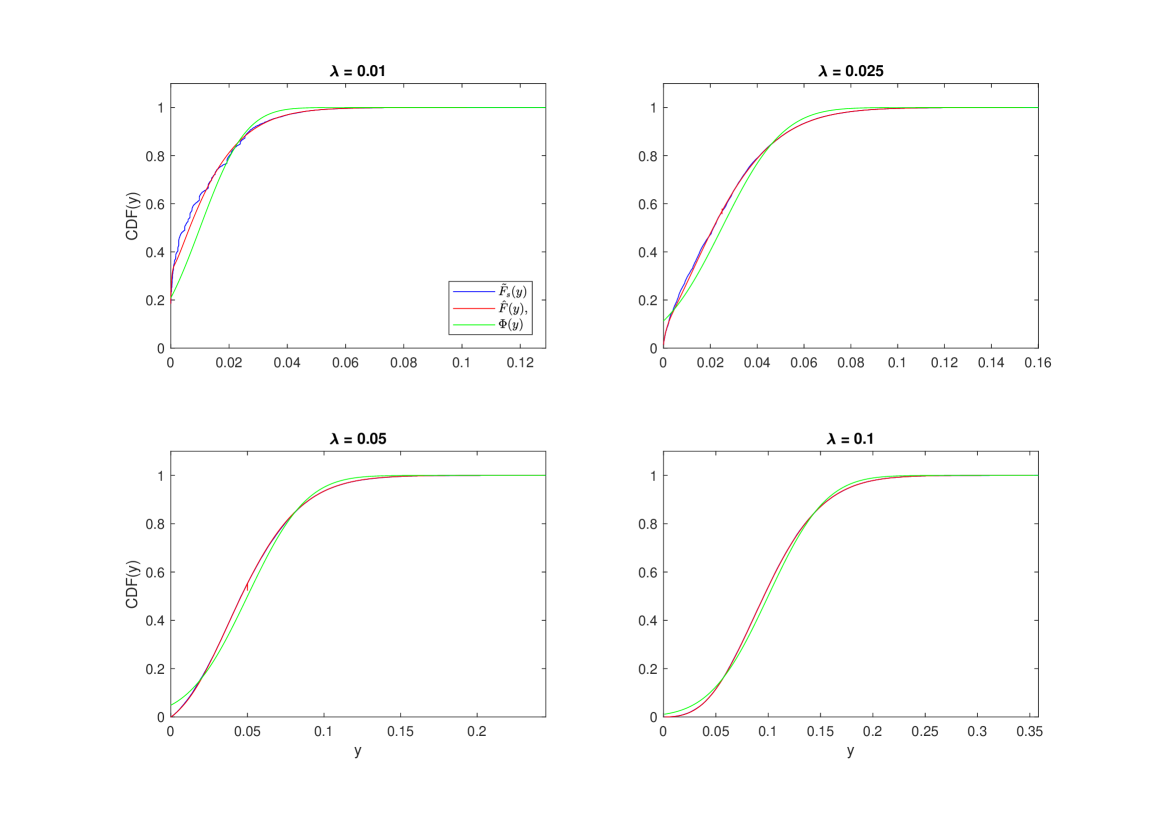
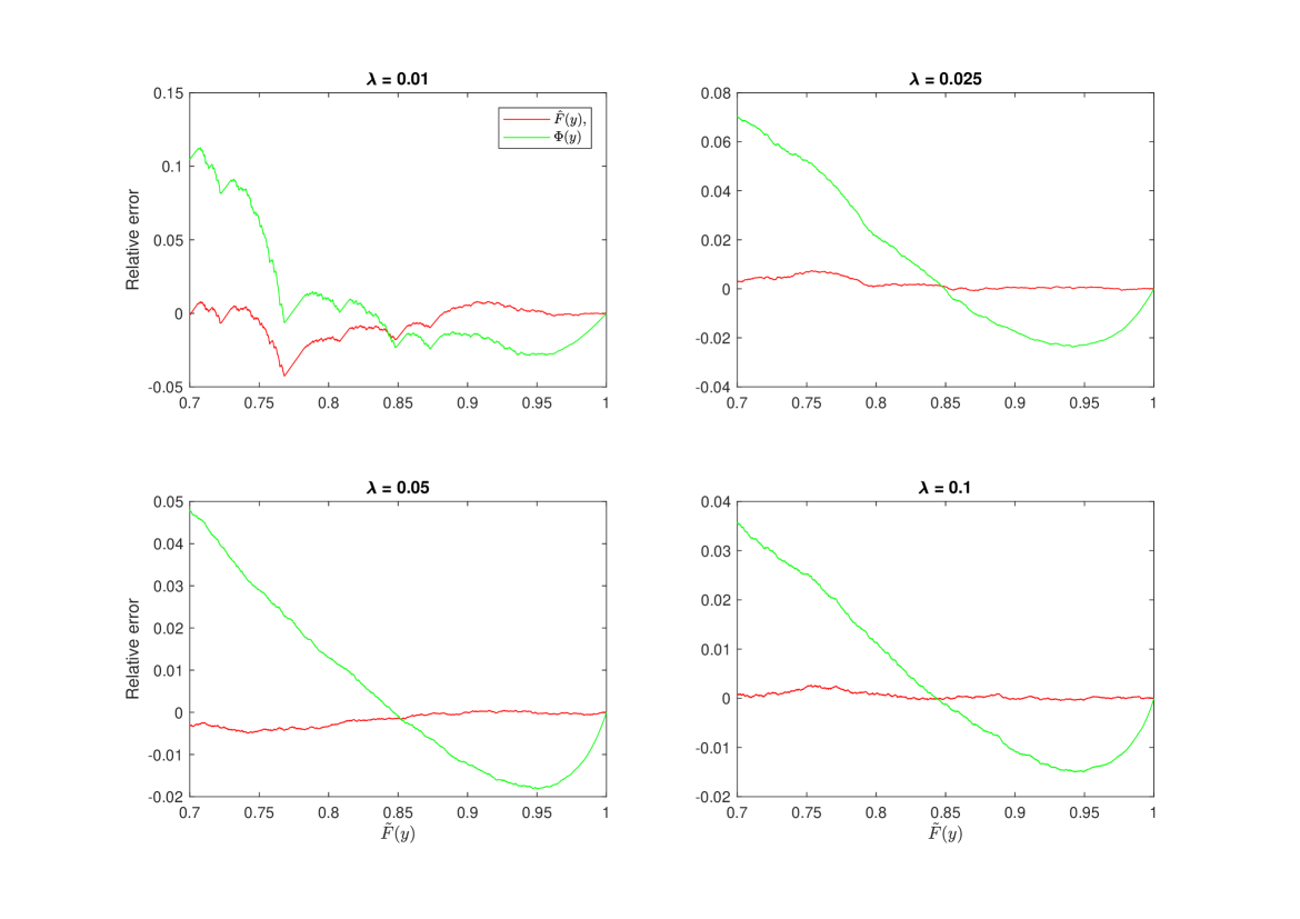
Figure 1 compares the histogram with the SA (normalized to unit area) to the PDF of the statistic for the central pixel of a set of MF filtered random realizations of a Poisson pixels noise process. Four values of the parameter , say , , , and (units in counts pix-1), have been considered. The MF has been computed assuming as a circular Gaussian with standard deviation pixels normalized to unit volume. For comparison, the Gaussian best fits are also shown. From these figures it is visible that better results are obtainable when increasing the values of . This is not an unexpected result since small values of imply that most of the pixels have zero counts, a few have one count and very few have larger counts. Especially for “narrow” signals , the consequence is a rough PDF for the statistic . However, in the case of , the top-right panel of Fig. 1 shows that, although the SA is not able to reproduce all the details of , it provides a good envelope resulting in a good approximation to the corresponding CDF. This is supported by Fig. 2 which compares the sample CDF with the corresponding to the PDFs in Fig. 1. The agreement is excellent. This is more evident in Fig. 3 where the relative errors are plotted versus for values of such as . This is a useful fact since in signal detection problems it is the complementary CDF and not the PDF which matters.
The SA does not work with very small values of . However, it is questionable that in situations of very low-number count regime the MF could be a useful approach. For example, in the case of a pixels map and , only pixels are expected with values greater than zero, i.e. only one pixel in each area of squared pixels. Under these conditions the use of the MF does not make sense since there is nothing to filter out. Moreover, the expected noise background should consist of bumps all with the same shape and amplitude. A more effective approach is based on the observation that the probability to have two counts in a pixel is of order of . Thereof, all the non-zero pixels are expected to have only one count. In addition, given that the probability of two pixels occupying adjacent positions is of order of , only four of them are expected to be neighboring. In other words, the detection of a signal can be claimed with high confidence in presence of pixels with counts greater than one and possibly contiguous with other non-zero pixels.
The conclusion is that, apart from extremely low levels of the noise background, the SA is able to provide excellent results. As visible in Figs. 1-3, this is not true for the Gaussian approximation. Hence, to test if after the MF filtering the value of a pixels is not due only to the noise, it is sufficient to check if with a prefixed .
6 Expected performances of the MF
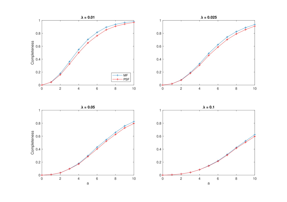
The excellent computation efficiency, but above all the good flexibility of the SA in the calculation of the with different noise levels and functional forms of , allow us to explore the expected performances of the MF in better detail than possible with an approach based on numerical simulations. In particular, in Ofek & Zackay (2017) the performances of the MF are compared to those of its most important competitor which is the point spread function filter (PSFF) technique where it is assumed that . One of the main reasons for such a comparison lies in the fact that in the case of a Gaussian additive white-noise the PSFF and the MF concide. Another reason is that even for relatively small values of the PDF of the Poisson noise can be reasonably approximated with a Gaussian. Moreover, under the conditions we are working under, the Poissonian noise level is constant across the background area but it changes only close to the signal position. However, since the MF is often used in situations where the amplitude of the signal is smaller than the level of the noise, in first approximation it can be assumed that . Hence, the noise can be considered of additive type with a constant level everywhere. In conclusion, there are situations where the PSFF can be an acceptable approximation to the MF. The results obtained by Ofek & Zackay (2017) indicate that in general the MF is superior to the PSFF for small values of and similar for larger values of this parameter. But, because of the very large number of numerical simulations necessary to fix a reliable detection threshold for each different experimental situation, their analysis is based on a few cases only. Here, we carry out a set of similar simulations with a larger combination of noise levels and signal intensities.
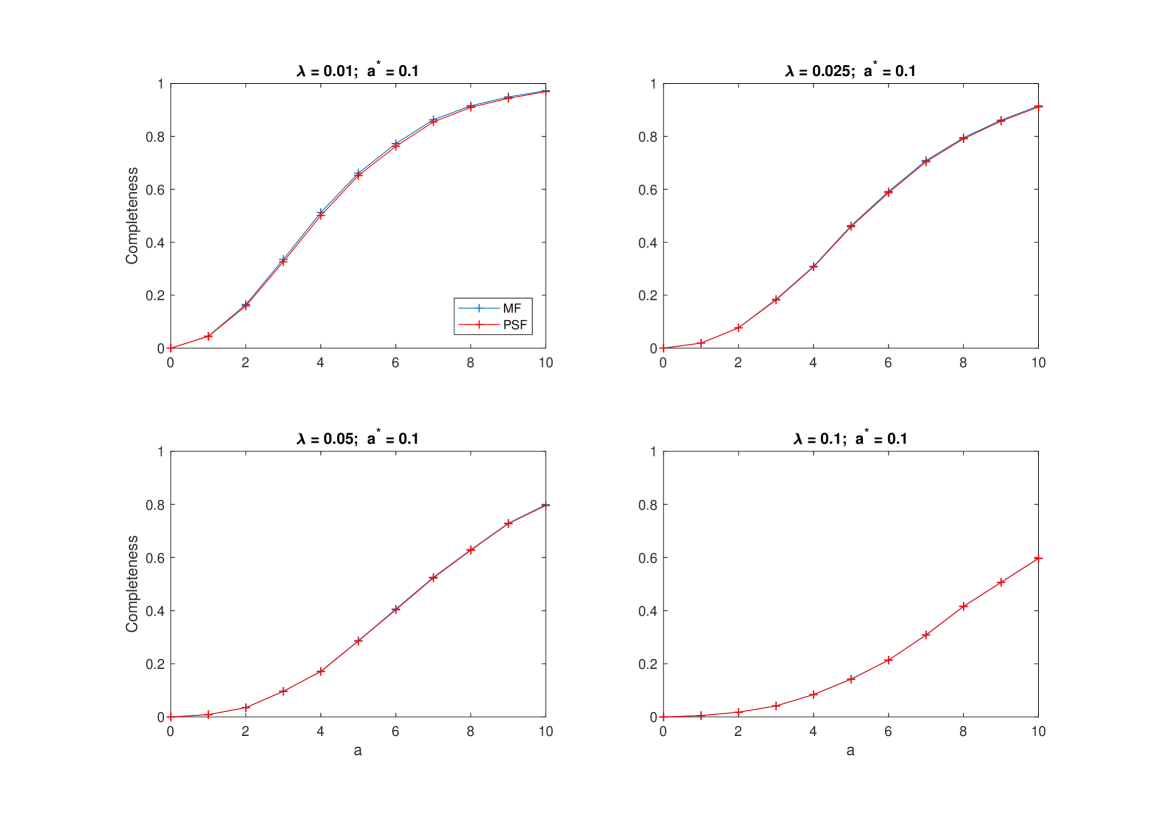
Our numerical experiments confirm the results of Ofek & Zackay (2017). This is shown by Fig. 4 where the completeness (i.e. the fraction of correctly detected signals) of the MF is compared with that of the PSFF for various combinations of and . It is visible as the results provided by the MF are effectively superior to those of the PSFF. However, the performances move closer and closer for increasing values of . In the experiments is a circular Gaussian with pixels, and the completeness has been estimated on the basis of simulated pixels maps assuming a detection threshold corresponding to .
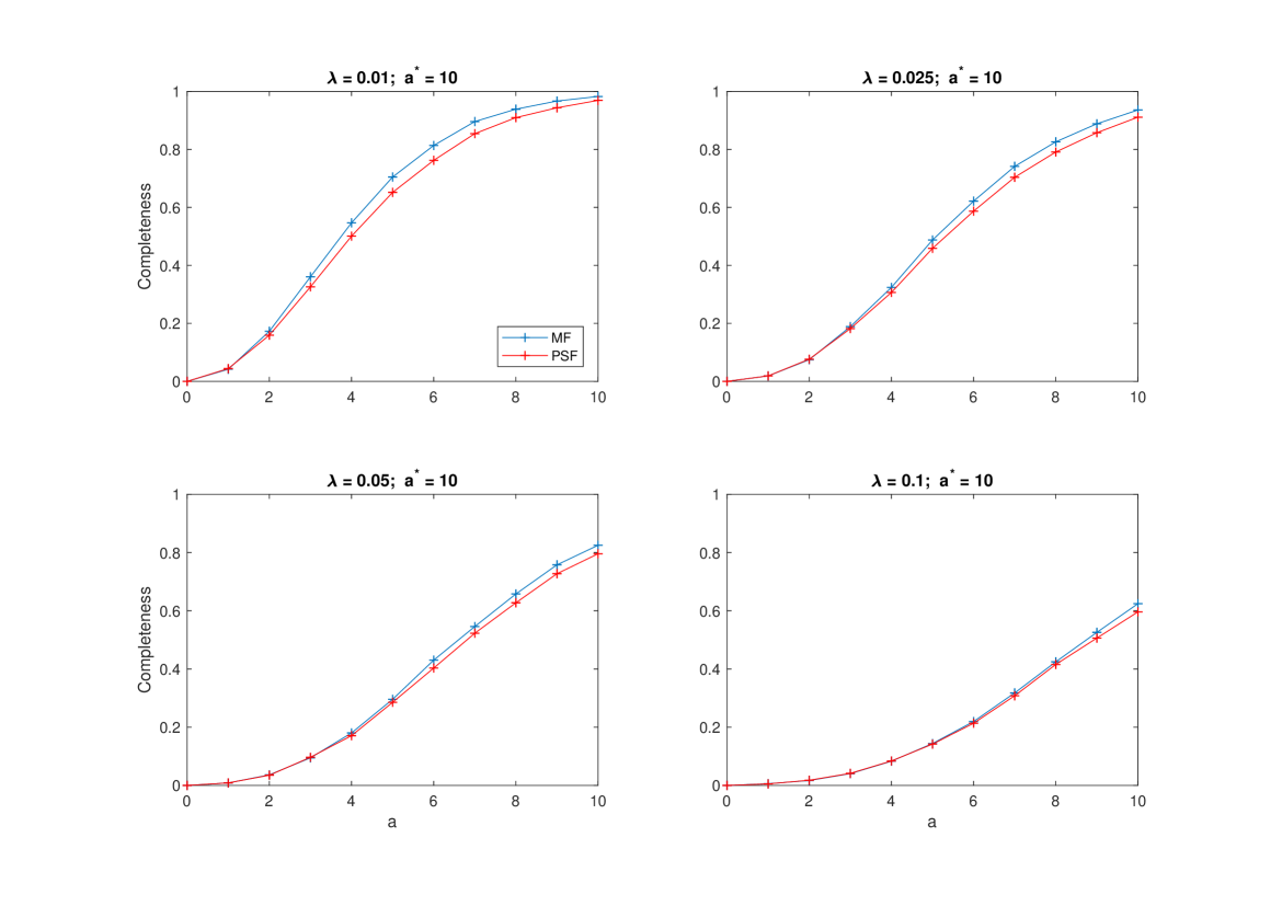
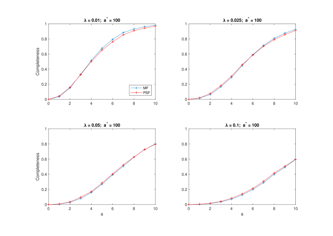
Although indicative, such experiments, as well those by Ofek & Zackay (2017), are affected by an important limitation: the comparison between the MF and the PSFF is done assuming that in the MF takes true values. But in real situations this information is not available. An example is sky maps containing point sources with different amplitude. For this reason, we have carried out another set of numerical experiments similar to the previous ones but using incorrect signal amplitudes . The results are shown in Figs. 5-7 for , , and . The indication that comes out from these figures is that, for a given value of , the performances of the MF effectively do not critically depend on the exact value of and, although less remarkably, tend to remain superior to those provided by the PSFF. Only values of very different from the true one determine an appreciable degradation of the results.
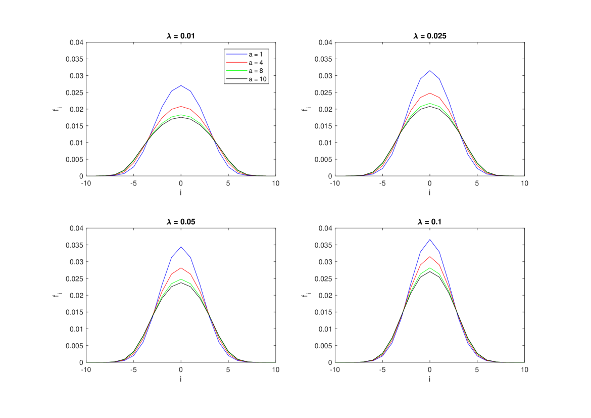
Finally, another indication which comes out from Figs. 5-7 is that it appears less harmful to use values of greater, rather than smaller, the true value. The reason of this fact can be deduced from Fig. 8 which shows the 1-D cut of the MF for different combinations of and . With fixed, it is evident that when increases the filtering action of the MF is stronger. This results in an over-filtered signal but also in a more robust attenuation of the noise. On the contrary, using an smaller that will result in an insufficiently filtered noise. The former situation appears preferable.
7 Shortcomings of the MF with Poisson noise
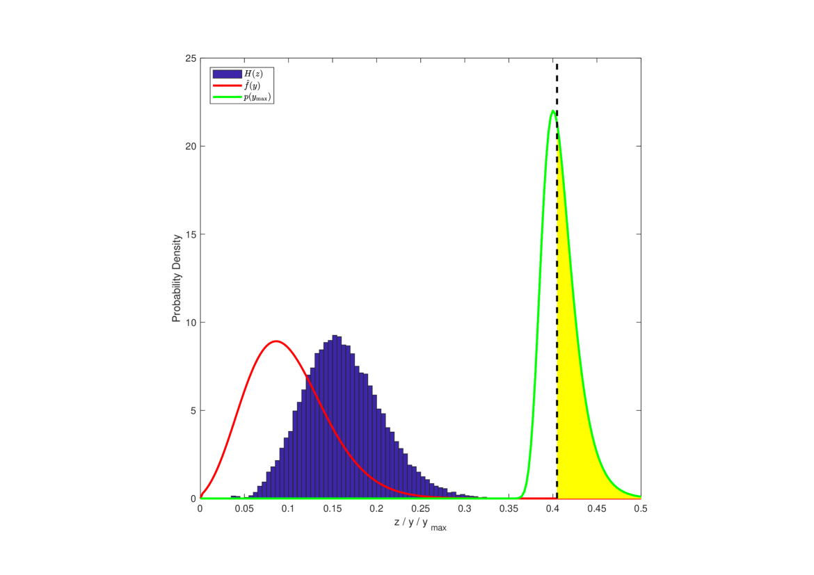
Thanks to the SA it is possible to find a partial solution to a still unsolved problem. In particular, the performances of the MF (5) have been tested under the implicit assumption that the position of within is known. In real situations this condition is rarely met (e.g. point sources in a two-dimensional map). The standard procedure to circumvent this issue is to cross-correlate with the MF and then to apply the detection test (4) to the resulting most prominent peaks. However, as shown in Vio & Andreani (2016) and Vio et al. (2017) for the Gaussian case, the PDF of the peaks of a random field is different from that of its generic points. Of course, the same holds also for the Poisson case. This is shown by Fig. 9 where the PDF of a pixels Poisson random field with and filtered by means of the MF in Eq. (5) with a circular Gaussian with pixels, is compared with the histogram of its peaks. It is evident that working with the peaks, and assuming the PDF for the the statistic in Eq. (12), may severely underestimate the with the risk of giving statistical significance to features that belong to the noise.
Contrary to the Gaussian noise (Cheng & Schwartzman 2015a, b), the PDF of the peaks is not available for the Poisson noise. Without it, a precise computation of the is not possible. Moreover, there is the additional difficulty that, if peaks are present in a MF filtered map, then a number among them is expected to exceed, by chance, the prefixed detection threshold. For example, if , then there is a high probability that a detection with a nominal equal to is spurious. Hence, the true has to depend on (look-elsewhere effect). The popular way-out to get around this issue is to assume as the PDF of the peaks (i.e. the peaks are regarded as generic points of the random field) and then to set with the number of independent pixels. If the noise is coloured, as it happens after the filtering operation, pixels are correlated with each other. Therefore, typically is smaller than and has to be estimated. Usually the estimation of is based on the correlation length of the template . The rational is that pixels with a mutual distance wider than the correlation length can be considered independent. For instance, in the case of a two-dimensional map and given by a circular Gaussian function with dispersion , Ofek & Zackay (2017) suggest that . This is to point out that such approach provides results which are only correct as an order of magnitude but no alternative is available if additional a priori information is missing.
In the present context, such procedures can be efficiently implemented by means of the order statistics, in particular by exploiting the statistical characteristics of the greatest value of a finite sample of identical and independently distributed (iid) random variables from a given PDF (Hogg et al. 2013). Under the iid condition, the PDF and the CDF of the greatest value among a set of independent pixels with PDF are given by
| (16) |
and
| (17) |
respectively. Hence, by assuming that the greatest value among a set of pixels coincides with that of a peak, a detection can be claimed when for a given peak it is .
This is an alternative way, though equivalent, to threshold the data which does not require the inversion of to fix the parameter corresponding to a given . In Vio et al. (2017) the quantity is called specific probability of false alarm (SPFA). The PDF for the numerical experiment of this section is also shown in Fig. 9 as well the corresponding to the largest peak observed in the map. We stress that in the case of large maps, an alternative based on numerical simulations is not viable.
8 Conclusions
In this paper we have introduced an efficient and effective implementation of the matched filter in the case of low-number count Poisson noise regime. We have shown that although the probability distribution and the cumulative distribution functions of the pixel counts after the MF filtering are not available they can be approximated with excellent results using the saddlepoint approximation method. With such techniques more accurate estimations of the probability of false detection or false alarm are obtained without making use of empirical or numerical methods.
Acknowledgements.
The authors warmly thank Martine Pelzer for her careful reading of the paper and correction of the English editing.References
- Briggs (2004) Briggs, J. 2004, Target Detection by Marine Radar (London: IET)
- Butler (2007) Butler, R.W. 2007, Saddlepoint Approximations with Applications (Cambridge: Cambridge University Press)
- Cheng & Schwartzman (2015a) Cheng, D., & Schwartzman, A. 2015a, Extremes, 18, 213
- Cheng & Schwartzman (2015b) Cheng, D., & Schwartzman, A. 2015b, arXiv:1503.01328 [math.PR]
- Paolella (2007) Paolella, M.S. 2007, Intermediate Probability, (Chichester: John Wiley & Sons Ltd)
- Hogg et al. (2013) Hogg, R.V., McKean, J.W., & Craig, A.T. 2013, Introduction to Mathematical Statistics (New York: Pearson)
- Kay (1998) Kay, S.M. 1998, Fundamentals of Statistical Signal Processing: Detection Theory (London: Prentice Hall)
- Levy (2008) Levy, B.C. 2008, Principles of Signal Detection and Parameter Estimation (New York: Springer Science + Business Media)
- Lugannani & Rice (1980) Lugannani, R., & Rice, S.O. 1980, Advances in Applied Probability, 12, 475
- Macmillan, & Creelman (2005) Macmillan, N.A., & Creelman, C.D. 2005, Detection Theory: a User’s Guide (Mahwah: Lawrence Erlbaum Associates)
- Minkof (2002) Minkof, J. 2002, Signal processing fundamentals and applications for communications and sensing (Boston: Artech House)
- Ofek & Zackay (2017) Ofek, E.O., & Zakay, B. 2018, AJ 155, 1690
- Osche (2002) Osche, g.R. 2002, Optical Detection Theory For Laser Applications (Oboken: Wiley-Interscience)
- Stewart (2006) Stewart, I.M 2066, A&A, 454, 1009
- Tuzlukov (2001) Tuzlukov, V.P. 2001, Signal Detection Theory (New York: Springer Science + Business Media)
- Vio & Andreani (2016) Vio, R., & Andreani, P. 2016, A&A, 589, A20
- Vio et al. (2017) Vio, R., Vergès, C., & Andreani, P. 2017, A&A, 604, A115
- Yao et al. (2013) Yao, K., Lorenzelli, F., & Chen, C.E. 2013, Detection and Estimation for Communication and Radar Systems (Cambridge: Cambridge University Press)
Appendix A A simple derivation of the saddlepoint approximation
Saddlepoint approximation (SA) is a powerful tool for obtaining accurate expressions of probability density functions and cumulative distribution functions. It can be derived in a number of ways. Most of them, however, are rather technical. Here, we provide an informal derivation due to Paolella (2007). A more technical and rigorous derivation can be found in Butler (2007).
As seen in appendix B, if is random variable with PDF , moment generating function (MGF) existing for with a neighborhood around zero, and cumulant generating function (CGF) , its mean and variance are given by and , respectively. With this premise, the derivation of the SA proceeds according to the following steps:
-
1.
A new random variable is defined having PDF
(18) for some ;
-
2.
the MGF and the CGF of are computed, respectively, as
(19) (20) The mean and the variance of are given, respectively, by and ;
-
3.
Fixed an arbitrary , is approximated by a Gaussian PDF with mean and variance . Here, and ;
- 4.
-
5.
The value of has to be determined in such a way that, for a fixed , is the best approximation to . In this respect, it is well known that the normal approximation to the distribution of a random variable is accurate near the mean of , but degrades in the tails. As a consequence, it is logical to choose a value of such as , i.e.
(23)
-
6.
Once has been fixed, the normal density approximation becomes and the approximation to simplifies to
(24)
The only critical point in this procedure is that has to be evaluated, via the solution of Eq. (23), for each where has to be computed. In general, this requires a numerical approach. However, for a fixed Eq. (23) has only one solution since it can be shown that is always a strictly convex function when evaluated over the converge interval of . Consequently, the mapping for into the support of the PDF is a bijection and thereof is strictly increasing (see pag. 6 in Butler 2007). Another question is that will not, in general, integrate to one, although it will usually not be far off. Therefore, it has to be numerically normalized.
Appendix B The moment and cumulant generating functions
Given a continuous random variable with probability density function and a positive number such that for the mathematical expectation
| (25) |
exists, then this expectation is called the moment generating function (MGF) of and is denoted by . The largest open interval around zero where for is referred as the convergence strip of . In the case is a discrete random variable with discrete PDF , becomes
| (26) |
The cumulant generating function (CGF) of is defined as
| (27) |
The terms in the series expansion are referred as the cumulants of so that the th derivative of evaluated at is , i.e.
| (28) |
It is straightforward to show that and , i.e. the first two cumulants provide the mean and the variance of .
One important property of the CGF is that in the case of a sequence of independent random variable for which has CGF determined over , then the CGF of is
| (29) |
In other words, the CGF of a sum of independent random variable is given by the sum of the respective CGFs.