Scalable high-resolution forecasting of sparse spatiotemporal events with kernel methods: a winning solution to the NIJ “Real-Time Crime Forecasting Challenge”

Abstract

We propose a generic spatiotemporal event forecasting method, which we developed for the National Institute of Justice’s (NIJ) Real-Time Crime Forecasting Challenge (National Institute of Justice, 2017). Our method is a spatiotemporal forecasting model combining scalable randomized Reproducing Kernel Hilbert Space (RKHS) methods for approximating Gaussian processes with autoregressive smoothing kernels in a regularized supervised learning framework. While the smoothing kernels capture the two main approaches in current use in the field of crime forecasting, kernel density estimation (KDE) and self-exciting point process (SEPP) models, the RKHS component of the model can be understood as an approximation to the popular log-Gaussian Cox Process model. For inference, we discretize the spatiotemporal point pattern and learn a log-intensity function using the Poisson likelihood and highly efficient gradient-based optimization methods. Model hyperparameters including quality of RKHS approximation, spatial and temporal kernel lengthscales, number of autoregressive lags, bandwidths for smoothing kernels, as well as cell shape, size, and rotation, were learned using crossvalidation. Resulting predictions significantly exceeded baseline KDE estimates and SEPP models for sparse events.

arXiv:1801.02858

, ,
and

t1Support was provided by the EPSRC (EP/K009362/1) and the European Research Council under the European Union’s Seventh Framework Programme (FP7/2007-2013) ERC grant agreement no. 617071. Source code to reproduce our results is available: https://github.com/MichaelChirico/portland.

1 Introduction

Figure 1: Early use of crime pin-maps at Scotland Yard. 1947 ©Illustrated London News Ltd/Mary Evans

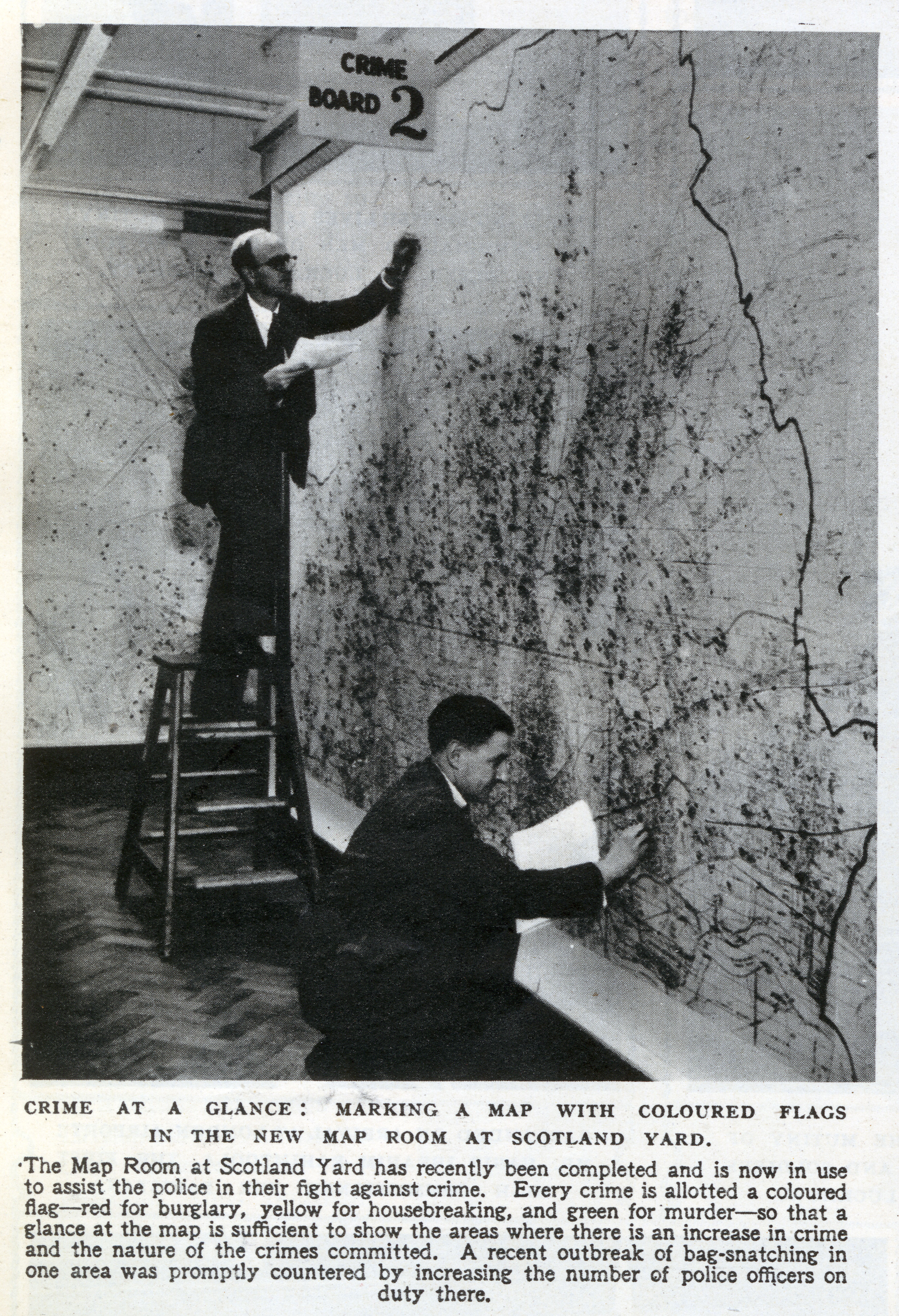
Spatiotemporal forecasting of crime has been the focus of considerable attention in recent years as academic researchers, police departments, and commercial entities have all sought to build forecasting tools to predict when and where crimes are likely to occur (Perry et al., 2013). The earliest crime forecasting tools consisted of nothing more than pin-maps (See Figure 1). Prior week’s crimes were mapped and qualitative assessments of density, location, stability and significance were made (Schutt, 1922).

Subsequent tools have adopted a range of different smoothing techniques to augment this method with kernel density estimation the most commonly used approach (Gorr and Lee, 2015; Porter and Reich, 2012; Chainey, Tompson and Uhlig, 2008a; Johnson et al., 2009). Many methods are model-driven, based on theories of crime causation (Caplan, Kennedy and Miller, 2011; Mohler et al., 2011). Some use log-Gaussian Cox Processes (LGCPs) (Rodrigues and Diggle, 2012; Shirota et al., 2017), while others use self-exciting point process models (SEPPs) (Levine, 2004; Liu and Brown, 2003; Taddy, 2010; Mohler et al., 2011; Rosser and Cheng, 2016) based on evidence of elevated levels of near-repeat victimization (Pease et al., 1998). Some use additional information, such as weather, demographics, and even social media (Wang, Gerber and Brown, 2012). Most simply use past events to forecast future events (Chainey, Tompson and Uhlig, 2008b; Kang and Kang, 2017), suggesting that methods that are effective at forecasting crime could readily be generalized to an increasing number of real-time spatiotemporal forecasting problems (Taddy, 2010). However, users of these methods often confront the question of which method to adopt and how to ensure optimal performance across a wide variety of settings.

In 2016 the National Institute of Justice (NIJ) announced the Real-Time Crime Forecasting Competition to test which forecasting models could most accurately predict out-of-sample crime hotspots in the City of Portland. This solicitation drew in a wide range of competitors. Teams were given five years of historical calls for service data from the Portland Police Bureau (PPB) and asked to submit predictions for the locations of the largest crime clusters in the subsequent weeks and months.

Our team (“Team Kernel Glitches”) tied for first place in the large organization category with wins across a range of categories. While our solution performed equally well on frequent and sparse crime forecasts and over short and long durations, it performed especially well, compared to competitors and contemporary methods, at forecasting sparse events over short durations. In describing our solution, we make the following contributions: we propose a flexible, generic, and scalable spatiotemporal forecasting model, casting the problem of spatiotemporal forecasting explicitly as a supervised learning problem, while incorporating existing and highly successful modeling approaches from the spatiotemporal statistics literature: Gaussian processes, autoregressive terms, kernel smoothing, and self-exciting point processes. This supervised learning setup provides a coherent framework for the time-consuming task of optimizing hyperparameters, while its modeling and inference scalability ensures that the model parameters themselves can be learned quickly enough to enable real-time forecasting. This approach achieves accuracy improvements well beyond those generated by existing best-practices in crime prediction (Chainey, Tompson and Uhlig, 2008b; Johnson et al., 2009).

The rest of this paper is laid out as follows. Section 2 describes our model. Section 3 describes the details of the NIJ competition. Section 4 reports competition performance. Section 5 concludes with a discussion of implications for future work on spatiotemporal prediction of crime and related phenomena.

2 Our model

2.1 Background

Previous methods for spatiotemporal forecasting of crime have either focused on highly flexible but relatively simple kernel density estimation techniques (Johnson et al., 2009; Gorr and Lee, 2015), where crime events are aggregated over time, smoothed over space, and used to predict crime patterns in the subsequent time period, or more complex and model-based approaches (Mohler et al., 2011; Rosser and Cheng, 2016). Recent work has demonstrated that Gaussian process modeling of crime data can produce highly accurate long-term forecasts by combining the benefits of nonparametric methods with the interpretability of additive methods (Flaxman, 2014). Subsequent work (Flaxman et al., 2015) has proposed that instead of specifying an additive kernel structure, it is is possible to learn it directly from the data, given enough data and a rich enough class of kernels. This assumes, however, that it is possible to perform inference with very large datasets, as the standard approach to Gaussian process inference requires matrix algebra to manipulate the multivariate Gaussian distribution in Eq. (A.4), requiring $\mathcal{O}(N^{3})$ time and $\mathcal{O}(N^{2})$ storage. We therefore first present the hypothetical model we would use if computational constraints were not a concern, then our actual model, which is an approximation to this model enabling application of this method to real-time rather than long-term forecasting problems.

2.2 Model specification

Our hypothetical model is a log-Gaussian Cox Process (LGCP). The LGCP is a doubly stochastic point process model. Given an observation window $W$ in space-time, we place a GP prior on the log-intensity $f(\bm{s})$ for any $\bm{s}\in W$. Let $N(\cdot)$ be a counting measure. For any space-time region $S\subset W$, $N(S)$ is a Poisson distributed random variable counting the number of points in $S$. Our hierarchical parameterization is as follows:

$$f \sim\mathcal{GP}(\mu,k_{\theta}(\cdot,\cdot))$$

$$N(S)|f \sim\mbox{Poisson}\left(\int_{S}\exp(f(\bm{s}))d\bm{s}\right)$$ (2.1)

We defer the specification of the mean $\mu$ and covariance kernel $k_{\theta}$ until later. For details on Gaussian processes see Appendix A.1.

Inference with the LGCP model is difficult because it is doubly intractable and existing approaches (Møller, Syversveen and Waagepetersen, 1998; Brix and Diggle, 2001; Cunningham, Shenoy and Sahani, 2008; Adams, Murray and MacKay, 2009; Teh and Rao, 2011; Diggle et al., 2013) are often limited to one dimension and small datasets. Lloyd et al. (2015) is a possible exception in that it points the way to a scalable stochastic variational inference approach.

To approximate this model we discretize. We specify a space-time grid partitioning $W$ into $N$ disjoints sets $S_{i}$, that is $W=\bigcup_{i=1}^{N}S_{i}$. As described below, this approach leads to a tractable model. Also, it is consistent with the design of the forecasting competition motivating our approach. For simplicity, let each grid cell $S_{i}$ be of equal volume $|S_{i}|=1$. The centroid of each grid cell is a latitude/longitude/timestamp triple $\bm{s}_{i}=(x_{i},y_{i},t_{i})$. The underlying point pattern is then represented as aggregate counts $o_{i}=N(S_{i})$ of the number of crimes per cell. Given the grid, the integral in Eq. (2.1) is approximated with a sum. When considering the entire observation window $W$, the approximation takes the following form:

$$\int_{W}\exp(f(\bm{s}))d\bm{s}\approx\sum_{i=1}^{N}\exp(f(\bm{s}_{i}))|S_{i}|=\sum_{i=1}^{N}\exp(f(\bm{s}_{i}))$$ (2.2)

In a Poisson process, conditional on the intensity, the random variables $N(S_{1})$ and $N(S_{2})$ are independent for $S_{1}\cap S_{2}=\emptyset$. Thus given the log-intensity $f$, each grid cell $S_{i}$ can be considered independently, so combining Eqs. (2.1) and (2.2) yields:

$$o_{i}|f\sim\mbox{Poisson}\left(\exp(f(\bm{s}_{i}))\right),~{}~{}\forall i=1,\ldots,N$$ (2.3)

This produces an iid likelihood (observation model) over all cells $i$, yielding the so-called computational grid approximation to the log-Gaussian Cox Process (Diggle et al., 2013; Flaxman et al., 2015).

In the function-space view of GPs, inference is performed about the function $f$ directly. Using the “kernel trick” (Schölkopf and Smola, 2002), all calculations can be carried out using a kernel $k_{\theta}$, evaluated at all pairs of $\bm{s}_{1},\ldots,\bm{s}_{N}$. However, to do this requires storing and manipulating an $N\times N$ covariance matrix $K$ at a cost of $\mathcal{O}(N^{2})$ storage and $\mathcal{O}(N^{3})$ computation (Rasmussen and Williams, 2006), which is infeasible for large $N$.

By contrast, the weight-space view of GPs (Rasmussen and Williams, 2006, Ch. 2) requires an explicit feature map $\phi(\bm{s})=k_{\theta}(\bm{s},\cdot)\in\mathcal{H}$ where $\mathcal{H}$ is the Reproducing Kernel Hilbert Space corresponding to the kernel $k_{\theta}$, with $\phi(\bm{s})^{\top}\phi(\bm{t})=k_{\theta}(\bm{s},\bm{t})$. Instead of learning $f$ directly (function space), for finite dimensional $\mathcal{H}$, a set of weights $\beta$ can be learned by considering the vector $\phi(\bm{s})$ as a set of basis functions. Thus we define $f(\bm{s}):=\phi(\bm{s})^{\top}\beta$ and observe that the weight-space view is equivalent to a linear model with a particular set of basis functions.

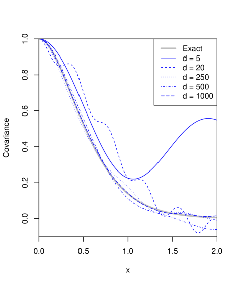
In practice, the weight-space view is not computationally tractable in the case of popular universal (Sriperumbudur, Fukumizu and Lanckriet, 2011) kernel choices like the Gaussian or Matérn kernel because the corresponding $\mathcal{H}$ is infinite dimensional. Unlike infinite-dimensional universal kernels, kernels corresponding directly to finite-dimensional RKHS are limited in their representational capacity, e.g. polynomial kernels of order $p$ only capture $p$ moments of a distribution. A solution can be found, following recent trends in the literature (May et al., 2019), using finite-dimensional approximations to universal kernels in the form of the random Fourier feature expansion (Rahimi and Recht, 2007) as described in Appendix A.2. For any kernel, this requires the selection of a dimension $d$ which determines the accuracy of the approximation $\hat{\phi}\in\mathcal{R}^{2d}$ where $\hat{\phi}(\bm{s})^{\top}\phi(\bm{t})\approx\phi(\bm{s})^{\top}\phi(\bm{t})=k_{\theta}(\bm{s},\bm{t})$. An example of our approximation is illustrated in Figure A1 where the Matérn-5/2 kernel is approximated using various values of $d$.

A finite dimensional $\hat{\phi}$ leads from the function-space view to the weight-space view (Rasmussen and Williams, 2006, Ch. 2), (Milton, Giorgi and Bhatt, 2019). To make the connection explicit we define a kernel $\hat{k}_{\theta}(\bm{s},\bm{t})=\hat{\phi}(\bm{s})^{\top}\hat{\phi}(\bm{t})$. Define a matrix $\Phi$ for observations $\bm{s}_{1},\ldots,\bm{s}_{N}$ with each row $\Phi_{i}=\hat{\phi}(\bm{s}_{i})^{\top}$. The function-space view on Gaussian process regression with covariance kernel $\hat{k}$ and a Gaussian likelihood is:

$$f \sim\mathcal{GP}(\mu,\hat{k}_{\theta}(\cdot,\cdot))$$

$$y|f,\bm{s}_{i} \sim\mathcal{N}(f(\bm{s}_{i}),\sigma^{2})$$ (2.4)

Eq. (2.4) is equivalent to Bayesian linear regression with $\beta\in\mathcal{R}^{2d}$ (where the term weight-space view comes from considering the parameter vector $\beta$ as “weights” to be learned):

$$\beta \sim\mathcal{N}(0,I)$$

$$y|\beta,\bm{s}_{i},\Phi \sim\mathcal{N}(\mu(\bm{s}_{i})+\Phi_{i}\beta,\sigma^{2})$$ (2.5)

For the present application, the data consists of count-valued observations, so we adopt a generalized linear modeling (GLM) framework and replace the Gaussian likelihood in Eq. (2.5) with the Poisson likelihood as in Eq. (2.3):

$$o_{i}|\beta,\bm{s}_{i},\Phi\sim\mbox{Poisson}\left(\exp(\mu(\bm{s}_{i})+\Phi_{i}\beta)\right)$$ (2.6)

It remains to specify the function $\mu$. In the spatial statistics literature, a linear model using spatially varying covariates is standard (e.g. (Diggle et al., 2013)), while $\mu=0$ is a common default choice in machine learning, though recent work has questioned this approach (Bhatt et al., 2017). We consider a different approach, based on prior work that has shown that using historical crime rates can be very effective in crime forecasting. Expanding upon prior KDE-forecasting methods that search a limited number of possible values and in line with the supervised learning framework discussed above, $\mu$ is parameterized as follows for $\bm{s}=(x,y,t)$:

$$\mu(\bm{s})=\sum_{j=1}^{p}\gamma_{j}\mbox{KDE}_{\lambda,j}(x,y,t)$$ (2.7)

where there are $p$ autoregressive lagged terms, each representing a spatial KDE for a given time period in the past and regression coefficients $\gamma_{j}$ are to be learned. $\mbox{KDE}_{\lambda,j}(x,y,t)$ is the kernel density estimator at location $(x,y,t)$ using a spatial Gaussian kernel $\kappa_{\lambda}$ with lengthscale $\lambda$:

$$\mbox{KDE}_{\lambda,j}(x,y,t)=\sum_{\{t_{i}~{}|~{}t-j\cdot D~{}<~{}t_{i}~{}\leq~{}t-(j-1)\cdot D\}}\kappa_{\lambda}((x,y),(x_{i},y_{i}))$$ (2.8)

where $D$ is the size of the temporal window in days.

Given the potential for a large number of parameters $\beta$ (the more random frequencies $d$ we choose for the random Fourier feature expansion, the better our approximation), the use of $\ell_{1}$ and $\ell_{2}$ regularization (as in the popular elastic net (Zou and Hastie, 2005)) provides a useful simplification.

Finally, our objective is to maximize the penalized log-likelihood of the Poisson distribution. Simplifying and dropping constant terms yields the following objective, with parameters $\beta$ and $\gamma$ and regularization hyperparameters $a$ and $b$:

$$\sum_{i=1}^{N} \left[o_{i}\left(\sum_{j=1}^{p}\gamma_{j}\mbox{KDE}_{\lambda,j}(x_{i},y_{i},t_{i})+\Phi_{i}\beta\right)-e^{\sum_{j=1}^{p}\gamma_{j}\mbox{KDE}_{\lambda,j}(x_{i},y_{i},t_{i})+\Phi_{i}\beta}\right]$$ (2.9)

$$-a(\|\beta\|_{1}+\|\gamma\|_{1})-b(\|\beta\|_{2}^{2}+\|\gamma\|_{2}^{2})$$

2.3 Inference

We learn the parameters $\beta$ and $\gamma$ by maximizing the objective in Eq. (2.9) using gradient ascent. The random Fourier feature approximation combined with linear regression leads to immediate speed-ups and memory savings: whereas full GP regression is $\mathcal{O}(N^{3})$ time and $\mathcal{O}(N^{2})$ storage, calculating the random features for $\Phi$ is $\mathcal{O}(Nd)$ for both time and storage. Given a fixed design matrix $\Phi$, ordinary linear regression requires calculating $\Phi^{\top}\Phi$ which is $\mathcal{O}(Nd^{2})$ time and $\mathcal{O}(d^{2})$ storage. Depending on how the lasso and ridge penalties are implemented, penalized linear regression can be very efficient, e.g. cyclical coordinate descent takes $\mathcal{O}(Nd)$ time for each update of all of the parameters (Friedman, Hastie and Tibshirani, 2010). The important point is that the overall running time is linear in $N$ rather than cubic, a significant savings in time. This approach is competitive with standard approaches to scalable inference in the spatial statistics literature (Sun, Li and Genton, 2012; Milton, Giorgi and Bhatt, 2019).

During competition, we performed optimization using the large-scale machine learning package Vowpal Wabbit (http://hunch.net/~vw). Vowpal Wabbit employs feature hashing (Weinberger et al., 2009) and online learning, which is even faster than the standard $\mathcal{O}(Nd^{2})$ approach to linear regression, allowing it to scale up to handle huge datasets. We fit the training dataset using default settings for the learning algorithm (a variant of online gradient descent), with at most 200 training passes (epochs) through the dataset. As a stopping criterion for convergence was applied, running times did not directly vary with dataset size. For any given set of hyperparameters (except the regularization parameters), a new dataset was produced and saved to disk, and then this model was fit across the full path of regularization parameters by repeatedly running Vowpal Wabbit. The entire process of dataset creation and multiple calls to Vowpal Wabbit usually took about half an hour, even with datasets as large as $N\approx 300k$ (1 week time horizon). All of our computation was carried out in a parallel cluster computing environment, with 8 Dell PowerEdge R630 nodes. Each node consisted of 2 $\times$ Intel Xeon E5-2690 v4 2.6 GHz, 14 Core CPUs, and 256 GB memory.

After fitting the model, we made predictions in the form of counts for the test data, and then calculate PEI for each year of data, where PEI is a forecasting accuracy metric used in the crime forecasting literature. To learn the hyperparameters we maximize average PEI. The hyperparameters related to our model are as follows: the number of random features $d$ in our feature expansion, the number of lags $p$, the size of the temporal window $D$, the spatial lengthscale for KDE $\lambda$ (with a Gaussian kernel), the lengthscale $\theta$ of the covariance kernel $k_{\theta}$ (we used a Matérn-5/2 kernel, a standard choice in spatial statistics (Guttorp and Gneiting, 2005)), and the amount of $\ell_{1}$ and $\ell_{2}$ regularization $a$ and $b$. In addition, there are competition-related hyperparameters that are learned, including: cell size, shape, grid rotation, and forecast area. We crossvalidated over a very large grid of hyperparameters, considering a range of values for each parameter and every possible combination of these values. As an alternative method to further explore the entire space of hyperparameter choices, we separately performed hyperparameter search using sequential Bayesian Optimization (O’Hagan, 1992; Snoek, Larochelle and Adams, 2012; Hennig, Osborne and Girolami, 2015). Having run both searches, we combined the results and chose the best sets of hyperparameters based on crossvalidated average PEI. Additional details are given in Appendix C.

2.4 Relationship with prior work

Supervised learning methods are widely used within non-spatiotemporal applications. However, they are less commonly used within the applied spatial (Heaton et al., 2018), time series (Makridakis, Spiliotis and Assimakopoulos, 2018), and crime forecasting domains. In crime forecasting, KDE-based forecasting approaches remain the most common forecasting techniques used (Gorr, Olligschlaeger and Thompson, 2003; Gorr, 2009; Chainey, Tompson and Uhlig, 2008a; Caplan, Kennedy and Miller, 2011; Berk et al., 2018). While small numbers of parameters may be user-selected and modified, these methods are commonly implemented absent any framework for maximizing the objective function of forecasting accuracy. Instead, practitioners modify parameters on an ad hoc basis, assuming that the resulting forecasts are a reasonable implementation of KDE methods. For a recent exception to this approach, see Rosser and Cheng (2016).

When prior work has sought to improve upon the performance of these less-than-optimized KDE forecasts, the principle area of focus has not been on scalable hyperparameter optimization, but instead on implementing model-based characterizations of underlying crime intensities. Some work has focused on modeling spatial and temporal range of crime decays (Johnson et al., 2009), but the Hawkes process has recently been the focus of significant attention in the crime forecasting literature (Ogata, 1988; Møller and Rasmussen, 2005; Mohler et al., 2011, 2013; Mohler, 2014; Rosser and Cheng, 2016; Loeffler and Flaxman, 2018). Both approaches seek to avoid a common feature of prior KDE methods which implicitly weight all prior events as equally informative with no attention to recency. However, the question of how to identify the optimal spatial and temporal range of crime decay is also not entirely addressed in these contributions.

The logic of our approach is that it combines state-of-the-art nonparametric spatiotemporal methods (Gaussian process regression), which fundamentally encode an assumption of spatial and temporal autocorrelation, with the most long-standing and widely used crime forecasting method (KDE surfaces) by defining sets of features for each. By placing these two sets of features into a penalized supervised learning framework for forecasting the intensity, and considering a large set of hyperparameters and training data, we hope to combine the benefits of nonparametric modeling, principally accuracy in the absence of a known best model, with the benefits of parametric modeling, principally model simplicity, to obtain good predictive performance on unseen data. For a discussion of the similarities of optimized KDE features and so-called “Hawkes features”, see Appendix A.3.

3 The competition

The goal of the NIJ Real-Time Crime Forecasting Competition was to forecast hotspots for several categories of calls for service to the Portland Police Bureau (PPB) in Portland, Oregon. Contestants submitted forecasts on (or before) February 28, 2017 for various time horizons starting on March 1, 2017 and extending as late as May 31, 2017. The hotspot predictions were scored on two metrics related to their accuracy. Contest rules required that contestants predict which of the 62,500 - 360,000 square foot cells within PPB’s 147.71 square mile service area would have the highest number of calls for service, with the total forecast area being no smaller than 0.25 square miles and no larger than 0.75 square miles, equivalent to forecasting 175–525 city blocks out of a total of 103,397 blocks. Prizes were given out for five different cumulative forecast periods (1 week, 2 weeks, 4 weeks, 8 weeks, 12 weeks), four different crime categories (burglary, street crime, theft of auto, all calls for service), and two different accuracy metrics.

Figure 2: The competition focused on four categories of crimes, ranging from the very abundant (All Calls for Service) to the very sparse (burglaries). Shown here are the locations of reported crimes in February 2016.

3.1 Data and Setting

The NIJ Real-Time Crime Forecasting dataset consists of 958,499 calls for service records from the Portland Police Bureau (PPB), representing calls to Portland’s 911 system requesting police assistance from March 1st, 2012 through February 28th, 2017. As shown in Figure 2, the four categories of crime, which themselves varied in the degree of internal heterogeneity, included burglary (burglary and prowling), street crime (ranging from disturbance and threats up to armed robbery and assault with a Firearm), theft of auto, and all calls for service.

3.2 Metrics

The simplest metric for evaluating the accuracy of crime forecasts is the “hit rate” (Chainey, Tompson and Uhlig, 2008a):

$$\mbox{Hit rate}=\frac{n}{T}$$

where $n$ is the number of crimes predicted and $T$ is the total number of crimes in that period in that area. Performance on this metric depends critically on the size of the forecasted area in addition to underlying crime densities and forecasting quality. In the case of the NIJ competition, this coverage area was between 0.2% and 0.5% of the City of Portland.

The NIJ competition focused on two alternatives metrics (Chainey, Tompson and Uhlig, 2008a; Hunt, 2016), with a goal of allowing for a comparison of hit rates across forecasts using different coverage areas. The first metric, the prediction accuracy index (PAI) (Chainey, Tompson and Uhlig, 2008a), is the ratio of the hit rate to the fraction of area covered:

$$\mbox{PAI}=\frac{\frac{n}{T}}{\frac{a}{A}}.$$

This metric directly incorporates the trade-off between hit rate and coverage, as in an ROC curve, into the score weighting.

The second metric, the prediction efficiency index (PEI), is the ratio of PAI to the hypothetically maximum PAI that could have been obtained using the chosen coverage area and discretization of space. Since the forecasting area is the same in both the actual and hypothetical maximum cases, this reduces to:

$$\mbox{PEI}=\frac{n\hfill}{n^{*}}.$$

where $n$ is the number of crimes occurring in predicted hotspots, and $n^{*}$ is the maximum number of crimes that could have been captured for the forecasted area.

While optimizing either metric will produce similar results some of the time, optimizing for PEI incurs a PAI penalty proportional to the marginal change in forecasted area divided by the marginal change in correctly forecasted crimes. Therefore, the optimal cell selection for maximizing PEI will often fail to maximize PAI. For the competition, we maximized the PEI metric. (For a result making the opposite choice, see Mohler and Porter (2018).)

3.3 Data for training and hyperparameter selection

For a given spatial grid size, we restricted our temporal windows to match the corresponding forecasting window. For example, for a one week forecasting window, the training data is aggregated to the weekly level. The training period consisted of each prior year’s aggregated counts excluding the corresponding time period being forecasted. This excluded period formed the validation period. We then created a single dataset using data from the union of all of the training and validation periods. Using this dataset, we forecasted hotspot maps for the five different validation periods, corresponding to the five different years of pre-2017 data available and calculated PEI for each. The average of this heldout PEI was then maximized to select the hyperparameters of the model.

4 NIJ Challenge Results

In this section we describe the performance of our method according to the scoring metrics of the NIJ challenge, assess its robustness, and investigate what features of the model contributed to its out-of-sample performance.

There were a total of 40 prizes awarded, one for each of the highest PEI and PAI scores in each crime category and forecasting window. Our team won a total of 9 prizes in the “Large Business” competition. As we focused on maximizing the forecasting performance on the out-of-sample PEI metric, most of our winning entries were in this category: all calls for service (1 week, 1 month, 3 months), burglary (1 week, 2 weeks), street crime (2 weeks), and theft of auto (1 week). In addition, we also had winning PAI entries for burglary (1 week and 2 weeks).

At the heart of our model was a hyperparameter search strategy, in which final models were selected from the union of all models explored by an exhaustive grid search coupled with a Bayesian Optimization designed to optimize forecasting accuracy. In practice, there were no consistently chosen hyperparameter values: the grid cells were sometimes small squares $250\mbox{ft}\times 250\mbox{ft}$ (the minimum area) or large squares $600\mbox{ft}\times 600\mbox{ft}$ (the maximum area) or large rectangles $800\mbox{ft}\times 450\mbox{ft}$ (also the maximum area). The coverage fraction ranged from the minimum (0.25 sq miles) to the maximum (0.75 sq miles). The lengthscales for space and time were highly varied, as were the number of KDE lags and the KDE bandwidth. The number of random Fourier features went as low as $d=5$, which means that the surface was a very crude approximation to a Gaussian process consisting of the sum of $10$ random sine and cosine functions, to as high as $362$, a much better approximation. In a minority of cases, no $\ell_{1}$ or $\ell_{2}$ regularization was needed, but most final models used at least some $\ell_{2}$ regularization. In a minority of cases (4 out of 20) the best hyperparameters turned out to be those found by Bayesian Optimization, while in all other cases, the best hyperparameters were those found by grid search. (See Table A1 for details.) The lack of overlap in optimal hyperparameter selection across competition categories both reinforces the importance of supervised learning optimization for forecasting accuracy and raises the question of whether other, possibly more uniform, hyperparameter choices might also exist.

We examine the distribution of all PEI values obtained in our grid search for each category/forecast window separately. For the 1 week theft of auto and burglary categories, 41% and 44% (respectively) of the possible hyperparameter combinations gave PEI scores of 0. This is strong evidence for the importance of an exhaustive hyperparameter search, at least for these sparse events. To further quantify this numerically, we calculate the z-score of the maximum PEI for the distribution of PEIs for each category/forecast window. Our winning theft of auto 1 week entry had a PEI z-score of 21, and our winning burglary entries had z-scores of 12.4 (1 week) and 11 (2 weeks), all results which are consistent with the idea that good forecasting accuracy requires an exhaustive hyperparameter search. The distributions for more abundant crime types did not yield such extreme z-scores: in the All Calls for Service category, the z-scores of the maximum PEIs ranged from 2.5 to 4.0. In the street crimes category the z-scores of the maximum PEIs ranged from 2.8 to 5.6. Thus for more abundant crime types a range of hyperparameters could produce similar results.

Figure 3: Competition Maximum PEI Performance Among All Competitors. Each column represents the highest level of forecasting accuracy achieved across all competitors for a particular combination of crime type and forecasting period. From left to right all calls for service, burglary, street crime, and theft of auto for 1 week, 2 weeks, 1 month, 2 months, and three months (also left to right).

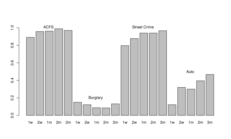
A final question concerning the competition is the maximum achievable level of forecasting accuracy. As shown in Figure 3, which depicts the maximum achieved PEI for all competitors, for high volume crimes, such as all calls for service, even a week’s worth of data is sufficient to achieve very high PEI scores (nearly 0.9) of the theoretical limit (1) for a one week prediction. Extending the cumulative forecast period leads to further improvements in forecasting accuracy, plateauing at 97%. Sizable sub-categories, such as street crimes, share this basic trajectory as well, suggesting that for high volume crimes over both short and medium-term horizons near limit and unity performance can be expected. For some sparse crimes, such as theft of auto, despite lower starting values, similar improvements in predictive accuracy can be seen as the forecasting windows are expanded, even if these improvements are not strictly monotonically increasing. Whether a longer horizon would lead to further improvements is unknown. However, for other sparse crimes, such as burglary, adding additional weeks of data to the forecast period does little to improve maximum achieved forecast accuracy. Reinforcing the idea that crime forecasting is not a single problem but several, only some of which are more accurately solved through the addition of more data.

4.1 Investigating method performance

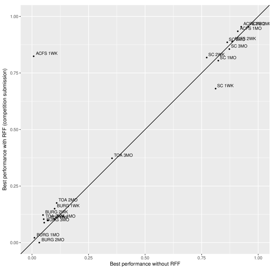
As discussed in Section 1, many crime forecasting implementations rely on KDE-type approaches. As our model included lagged KDE terms, we expected to always perform as well as a KDE-type baseline. As a post-competition check, we fit a model with just one KDE lag, corresponding to a KDE-type baseline, and fixed parameters according to common practice (Chainey and Ratcliffe, 2005) and found that our model was better than this baseline 90% of the time (18 cases out of 20) on the true out-of-sample forecasted data with an average absolute improvement of 0.16 for the PEI scoring metric. The improvements were most notable for sparse crimes and short time-horizons, as the baseline model often identified no correct theft of auto or burglary hotspots (Figure 4). Interestingly, for the two forecasts for which simple KDE outperformed our model (e.g., burglary 2m and 3m), hyperparameters for the model were selected using Bayesian Optimization rather than grid search, suggesting that BO will not always give the optimal set of parameters.

Figure 4: KDE Baseline (x-axis) compared to Full Model (y-axis). The Full Model out-performed the KDE Baseline Model in 18 out of 20 forecast problems. The average out-of-sample performance improvement of the Full Model over the KDE Baseline Model was 0.16 on the PEI scoring metric. BURG = burglary, SC = street crime, TOA = theft of auto, ACFS = all calls for service.

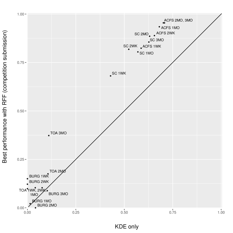
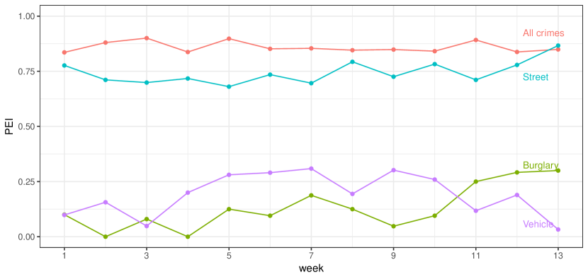
Comparing the full method, which combines lagged KDE terms and a Gaussian process surface, to a model without the Gaussian process surface, the full model gave better PEI results 75% of the time. The average absolute improvement was 0.05. Thus, although the full model is an improvement, the improvements are not as dramatic as going from a simple KDE to a lagged KDE model with kernels optimized for forecasting accuracy. This result suggests that for many models, especially ones predicting sparse events (as depicted in Figure 5), the routine variation in performance is sufficient to swamp the benefits of using Gaussian process surfaces or other complex methods. Instead, considerable portions of achievable performance improvements can be realized by optimizing the parameters of simpler methods, such as lagged KDEs.

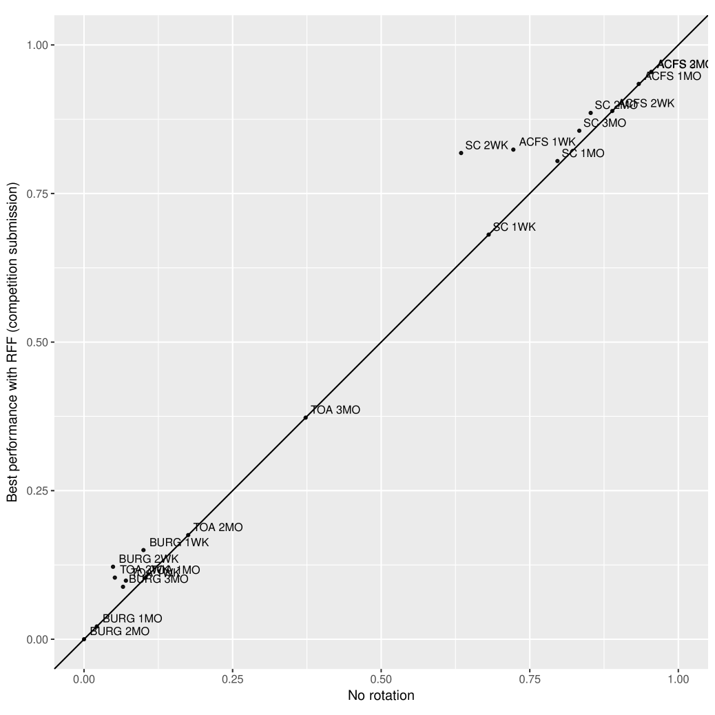
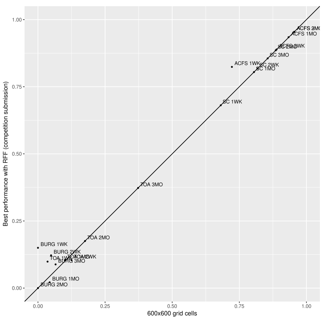
Rosser et al. (2016) recently demonstrated that due to geocoding, non-cardinal land use, and other related factors, a non-standard alignment could improve predictive accuracy in crime forecasting. In the present application, we explored altering the rotation of the entire tessellation and the dimensions of the cell rectangles. With improved performance of only 0.029 on the PEI scoring metric for a freely-rotated model when compared to the best performing non-rotated model, rotation does not appear to be a major contributor to overall performance. However, certain crime categories and forecast windows can be observed to benefit more substantially. A similar result can be observed for altering cell dimensions, which only improves overall performance on the PEI scoring metric by 0.019 when compared to a conventionally used 600x600 ft rectangle. (See Figures A2–A4 for more details.) These results parallel previous findings that showed the limited return on the inclusion of non-auto-regressive information (Wang, Gerber and Brown, 2012; Gerber, 2014).

The sparseness of several of the forecasted incidents and recent findings on lack of robustness of forecasting models (Rosser and Cheng, 2016) suggests that it is worthwhile to examine the stability of the model’s performance over multiple periods. To accomplish this, the 13 week competition period (March through May 2017) was split into 13 one-week forecast periods and a one-week rolling forward prediction was made for each week. The resulting predictions, as seen in Figure 5, manifest variability consistent with the stochastic events being predicted. However, these rolling-forward predictions provide little evidence of over-fitting to the first out-of-sample time period, even for the sparsest of incidents. They instead suggest, at least for settings like the competition, that the short-term accuracy improvements are robust and stable.

Figure 5: Rolling Forecast. The 13 week competition period (March through May 2017) was split into 13 one-week forecast periods and a one-week rolling forward prediction was made for each week using the competition model trained to predict only the first out-of-sample week.

Alongside sub-model component performance and model stability, a final area of interest is method error. Figure 6 (left) shows the actual performance of the full forecasting model for a high volume crime category (ACFS) and a middle-range forecasting period (1 month). Polygons that were correctly forecast as the highest possible crime count polygons are in green. Polygons incorrectly forecast to not be hotspots are in red. And polygons that were incorrectly predicted to be the highest possible crime count polygons are depicted in blue. Crimes are black dots. The largest single cluster of hotspots for all calls for service can be seen downtown. However, the model slightly over-invested in this section of Portland. As can be seen in the inset, hotspots just across the Willamette River had more crimes reported over the relevant forecast window. In practice, most of these misses were relatively small, with “false negatives” only slightly “hotter” than the corresponding “false positive” cells (e.g., 44 crimes in a FN cell versus 39 crimes in a FP cell).

Figure 6: Left: all calls for service 1 month. Correctly forecast polygons are in green. “False negative” polygons are in red. “False positive” polygons are depicted in blue. Crimes are black dots. Right: burglary 1 week. Forecasted burglary cells are depicted with boxes. Actual burglaries are depicted by blue x’s. Boxed x’s indicate a successful prediction. Empty boxes indicate a “false positive” prediction.

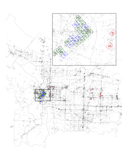
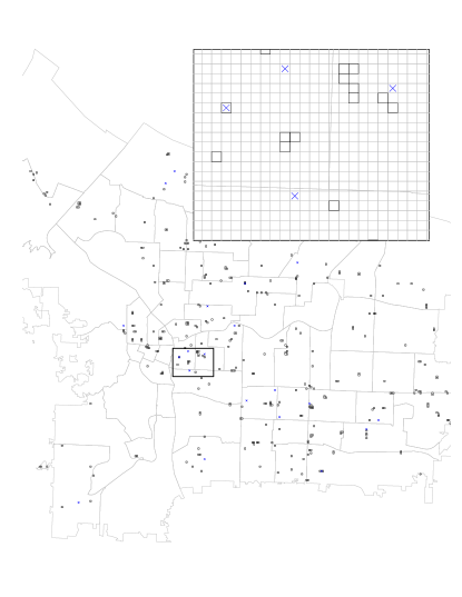
Figure 6 (right) show the actual performance of the model for a sparse crime category (burglary) and a short-range forecasting period (1 week). Forecasted burglary cells are depicted with boxes and actual burglaries are depicted by blue x’s. Boxed x’s indicate a successful prediction while empty boxes indicate a “false positive” prediction. The absence of large-scale clustering is quite visible in both the dispersion of the burglaries throughout Portland and in the similarly dispersed allocation of predictions. As can be seen in the inset, a successful prediction was accompanied by several near misses in the vicinity, including one near-miss off by only a single cell. Predicting sparse crimes, while more difficult than predicting concentrated crimes, is still achievable and with accuracy levels not previously seen with other conventional forecasting methods.

5 Discussion

Real-time spatiotemporal forecasting is an area of increasing interest. Yet many common approaches, such as kernel-smoothing based on fixed bandwidths and cell sizes, can be quite limited in their out-of-the-box accuracy, especially for sparse events. Past work (Johnson et al., 2009) has reported 1-week burglary forecasting accuracy of 10% at 1.3% of coverage area and 25% of burglaries at 5% of coverage area using near-repeat models with baseline KDE models producing 1-week accuracy of 10% at 2% coverage and 25% at 6.5% coverage. Mohler et al. (2011) report 5% accuracy for daily predictions at comparable coverage levels. By comparison, using the described methods, median 1-week burglary accuracy of 10% was achieved with a coverage area of 0.5% and 50% of the time 25% forecasting accuracy was achieved at 0.5% coverage.

These results build upon prior work exploring parameter tuning (Chainey, 2013; Rosser and Cheng, 2016) and reinforce three points. First, it appears that simple but well-tuned models incorporating lagged kernel smoothing can achieve many of the benefits commonly associated with more complex methods. This conclusion stems from the recognition that parameter optimization, particularly in the case of kernel smoothing, is a re-weighting of different spatiotemporal portions of an auto-regressive process for forecasting accuracy. Second, the poor performance of conventional kernel estimators with parameters set based on rules-of-thumb, suggests that many existing crime forecasting implementations are not as accurate as they could be. Third, while some parameters are more important than others, no one parameter is universally better and as such, supervised learning will likely be a continuing feature of spatiotemporal crime forecasting.

While the results reported here suggest that forecasting the hottest high volume crime hotspots can be done with great accuracy using a variety of techniques, the same cannot be said for sparse events, at least not yet. This leaves as an open question whether rare crime events are intrinsically harder to forecast due to random error or are simply harder because of insufficient training data. The fact that some rare crime forecasts saw no improvement in forecasting accuracy despite the addition of more training data and larger cumulative forecasting windows could be considered suggestive evidence that there may be a signal limit for this type of event. However, refitting our models in other settings would shed further light on this question, as would the inclusion of additional predictors. For example, $\mu$ based on the kernel density estimates of other types of crimes, inspired by criminology research on “leading indicators” of crime (Cohen, Gorr and Olligschlaeger, 2007).

Another question not answered by these results is why this method’s performance was not more uniform. One possible answer is that the methods described in this paper simply do a better job at forecasting certain types of events over certain forecasting windows. Another possibility is that incomplete grid-search of hyperparamaters during competition led to the use of sub-optimal parameters for certain forecasting sub-tasks. A final possibility is that the close performance of competitors, on at least some forecasting tasks, achieved near limit forecasting performance using known methods and data. In future work in other settings, these possibilities could more readily be teased out.

Pending completion of this research, the absolute performance of different methods in this competition also raises the policy question of what is an acceptable level of accuracy for any crime forecasting method to be used?

In recent years, crime forecasting tools have been a supplement or replacement for traditional crime analysis (Mohler et al., 2015), with applications to police deployment, enforcement actions targeted at particular individuals or places (Lum and Isaac, 2016; Perry et al., 2013), as well as non-enforcement notification strategies (Groff and Taniguchi, 2019). These applications, especially those involving law enforcement activity, have elevated concerns about fairness in criminal justice decision-making, leading to a vigorous debate about definitions of algorithmic fairness (Berk et al., 2018; Corbett-Davies et al., 2017; Mitchell, Potash and Barocas, 2018). While fairness is an important debate, we have focused instead on accuracy, as this is a necessary precondition to considerations of fairness (Dressel and Farid, 2018; Rudin and Ustun, 2018). As the results of our research suggest, opportunities for large gains in accuracy exist through the use of standard machine learning frameworks and spatial statistical methods.

Appendix A Scalable Gaussian processes

A.1 Gaussian processes

Following Cressie and Wikle (2011), we use Gaussian processes as the fundamental modeling approach for spatiotemporal data. In the particular case of point pattern data such as crime events, we follow Diggle et al. (2013) in considering the log-Gaussian Cox Process.

A Gaussian process is a stochastic model which can be used as a nonparametric prior over functions $f$. See Rasmussen and Williams (2006) for a comprehensive introduction. $f$ is defined on some index set $\mathcal{X}$ and for our purposes we will assume that $f$ is real-valued, so $f:\mathcal{X}\rightarrow\mathcal{R}$. $f$ is parameterized by a mean function $\mu$ and a covariance kernel function $k(\cdot,\cdot)$:

$$f\sim\mathcal{GP}(\mu,k(\cdot,\cdot))$$ (A.1)

meaning that:

$$E[f(x)] =\mu(x)$$ (A.2)

$$\mbox{Cov}(f(x),f(x^{\prime})) =k(x,x^{\prime})$$ (A.3)

The defining feature of a Gaussian process is that at any finite set of indices $x_{1},\ldots,x_{n}\in\mathcal{X}$, the distribution of the vector $[f(x_{1}),\ldots,f(x_{n})]^{\top}$ is a multivariate Gaussian:

$$[f(x_{1}),\ldots,f(x_{n})]^{\top}\sim\mathcal{MVN}([\mu(x_{1}),\ldots,\mu(x_{n})]^{\top},K)$$ (A.4)

where the covariance matrix $K_{ij}=k(x_{i},x_{j})$.

Gaussian processes are often described as a nonparametric model, since the number of parameters grows with the sample size, with attractive posterior consistency results in a simple regression setting (Choi and Schervish, 2007), and as part of a Cox survival model (Fernandez and Teh, 2016).

A.2 Scalable kernel methods

The matrix algebra operations required for calculations involving multivariate Gaussians are not scalable to large datasets. Practitioners face the same issue when applying nonlinear kernel methods (Schölkopf and Smola, 2002), as they rely on the calculation and manipulation of an $n\times n$ Gram matrix, which corresponds exactly to the covariance matrix parameterized by the covariance kernel in Gaussian processes. While a variety of approaches have been proposed to alleviate this computational difficulty (for a comprehensive comparison in the spatial setting, see Heaton et al. (2018)), we consider random Fourier features (Rahimi and Recht, 2007, 2008) due to the simplicity with which it can be embedded within a larger supervised learning framework.

Random Fourier Features are a randomized approximation yielding a finite-dimensional feature mapping (and corresponding finite-dimensional Reproducing Kernel Hilbert Space) which approximates the original kernel. Proposed in 2007 (Rahimi and Recht, 2007) and marketed as only requiring 3 lines of MATLAB code to apply, the authors won a “Test of Time Award” at NIPS in 2017 for their widespread applicability and elegance.

Recall Bochner’s theorem (for a precise statement in multiple dimensions see (Stein, 1999, p. 24)), which establishes a one-to-one correspondence between a stationary kernel $k(x_{i},x_{j})=\kappa(x_{i}-x_{j})$ and a positive finite measure $\Lambda$. In particular, $\kappa$ is the Fourier transform of $\Lambda$:

$$\kappa(x-y)=\int_{\mathcal{R}}e^{i\omega^{\top}(x-y)}d\Lambda(\omega)$$ (A.5)

Recognizing that this infinite dimensional integral is an expectation over the measure $\Lambda$ suggests that it can be approximated using Monte Carlo sampling. After normalizing appropriately, we treat $\Lambda$ as a pdf and consider iid samples:

$$\omega_{1},\ldots,\omega_{d}\sim\Lambda(\omega)$$ (A.6)

Then we have the following approximation:

$$\kappa(x-y) \approx\frac{1}{d}\sum_{j=1}^{d}e^{i\omega_{j}^{\top}(x-y)}$$ (A.7)

$$=\frac{1}{d}\sum_{j=1}^{d}\cos(\omega_{j}^{\top}(x-y))+i\sin(\omega_{j}^{\top}(x-y))$$ (A.8)

$$=\frac{1}{d}\sum_{j=1}^{d}\cos(\omega_{j}^{\top}x)\cos(\omega_{j}^{\top}y)+\sin(\omega_{j}^{\top}x)\sin(\omega_{j}^{\top}y)$$ (A.9)

$$=\langle\Phi(x),\Phi(y)\rangle$$ (A.10)

Since we know that the kernel is real-valued, in line (A.9) we ignore the imaginary component and expand using the trigometric identity for $\cos(\alpha+\beta)$. We can now define an explicit feature mapping $\Phi:\mathcal{X}\rightarrow\mathcal{R}^{2d}$ consisting of the following pairs of elements concatenated together:

$$\Phi_{j}(x)=\frac{1}{\sqrt{d}}\left(\begin{array}[]{c}\cos(\omega_{j}^{\top}x)\\ \sin(\omega_{j}^{\top}x)\end{array}\right)$$ (A.11)

Figure A1: We approximate a Matérn 5-2 with varying number of random Fourier features. The approximation becomes more and more exact as the number of features increases.

The elegance of random Fourier features is that in a supervised learning setting with $n$ observations and $p$ covariates with design matrix $X\in\mathcal{R}^{n\times p}$, we can immediately consider introducing kernel-based nonlinearities, without changing our learning approach, simply by transforming our design matrix into $[\cos(X\Omega^{\top})\quad\sin(X\Omega^{\top})]$ for a set of random frequencies $\Omega\in\mathcal{R}^{d\times p}$ (here, $\cos(A)$ is the element-wise computation of cosine on $A$). In homage to the three lines of MATLAB code, three lines of R code are shown below to transform a design matrix X into a new design matrix Phi assuming a squared exponential kernel with lengthscale 1, $k(x,y)=\exp(-.5\|x-y\|^{2})$. In our space-time setting, X has 3 columns giving the x, y, and t coordinates of the observations, but it could also include covariates if available.

Omega = matrix(rnorm(d*ncol(X)), d)
Proj = X %*% t(Omega)
Phi = cbind(cos(Proj), sin(Proj)) / sqrt(d)

Changing the covariance kernel’s lengthscale corresponds to changing the variance of the normal distribution. Using a Matérn kernel instead of a squared exponential requires sampling from a Student-t distribution instead of a normal distribution. At this point, any (suitably regularized) linear learning method can be applied to Phi: ridge regression with Phi is an approximation to kernel ridge regression with X; Bayesian linear regression with Phi is an approximation to Gaussian process regression with X.

As shown in Figure A1, a larger number of random features $d$ increases the accuracy of the approximation.

A.3 Hawkes features vs. KDE features

Our approach is similar to the “Hawkes features” used by Mohler and Porter (2018). However, as detailed below, both this previous work and ours are actually akin to the little studied nonlinear Hawkes process, rather than the more standard linear Hawkes process. The conditional intensity function used in a spatiotemporal linear Hawkes process takes the following form:

$$\lambda(x,y,t)=\lambda_{0}(x,y,t)+\sum_{\{i|t_{i}<t\}}k_{t}(t_{i},t)\cdot k_{s}((x_{i},y_{i}),(x,y))$$ (A.12)

where the first term is an underlying (endogeneous) intensity and the second term is the self-excitatory component.

We argue that in the supervised learning framework of training a model to predict the future given the present, the main distinction between an unweighted KDE and the Hawkes process disappears. The reason is that in the supervised framework, the lagged KDE features only have access to past events, so the intensity cannot rise before an event occurs, i.e. the directionality of time is enforced.

As defined in Eq. 2.8, $\mbox{KDE}_{\lambda,1}(x,y,t)$ is the lag-1 spatial kernel density estimator at location $(x,y)$ using data with time labels $\in[t-D,t]$, i.e.:

$$\mbox{KDE}_{\lambda,1}(x,y,t)=\sum_{\{i|t_{i}\in[t-D,t]\}}k_{s}((x_{i},y_{i}),(x,y))$$ (A.13)

If we consider Eq. (A.12) and the special case in which

$$k_{t}(t_{i},t)=\begin{cases}1~{}\mbox{if}~{}t_{i}\in[t-D,t]\\ 0~{}\mbox{otherwise}\end{cases}$$ (A.14)

the KDE feature is equivalent to the self-excitatory term in the Hawkes process conditional likelihood. This result makes sense in a supervised learning framework, in which the KDE values are computed ignoring future data (from the point of view of the features, the future has not occurred yet).

Note, however, beyond the particular kernel choice and lack of a time component, there is another major distinction between prior and present work: the log link function in our GLM framework implies that instead of these features contributing additively to the intensity, the exponential of their sum contributes to the intensity, or equivalently the product of exponentials. This is analogous to the rather exotic “nonlinear” Hawkes process (Gerhard, Deger and Truccolo, 2017; Carstensen et al., 2010; Zhu, 2013), where the effect of past events on the present intensity is multiplicative, rather than additive, and for which stability results are not well-established. This distinction applies to Mohler and Porter (2018) as well, due to the inclusion of the logistic link function.

The kernel in Eq. (A.14) is rather simplistic, suggesting an obvious extension to our method of including a more interesting temporal kernel in the KDE features of Eq. (A.13) and possibly also for other lags as in Eq. (2.8). It would be sensible as well to consider the more standard linear Hawkes formulation, which is known to be stable, instead of the nonlinear version considered here.

Appendix B Supplementary Results

Figure A2: Model Omitting Random Fourier Features (x-axis) compared to Full Model (y-axis). The Full Model out-performed the Model Omitting Random Fourier Feature in 15 out of 20 forecast problems. The average out-of-sample performance improvement of the Full Model over the Non-Rff Model was 0.05 on the PEI scoring metric. BURG = burglary, SC = street crime, TOA = theft of auto, ACFS = all calls for service.

Figure A3: Model Omitting Grid Rotation (x-axis) compared to Full Model (y-axis). The Full Model out-performed the Model Omitting Grid Rotation in 10 out of 20 forecast problems. The average out-of-sample performance improvement of the Full Model over the Non-Rotated Model was 0.029 on the PEI scoring metric. BURG = burglary, SC = street crime, TOA = theft of auto, ACFS = all calls for service.

Figure A4: Model with Fixed Grid Cells (x-ais) compared to Full Model (y-axis). The Full Model out-performed the Model with Fixed 600x600 ft cells in 6 out of 20 forecast problems. The average out-of-sample performance improvement of the Full Model voer the Fixed Cell Model was 0.019 on the PEI scoring metric. BURG = burglary, SC = street crime, TOA = theft of auto, ACFS = all calls for service.

Appendix C Hyperparameter choice

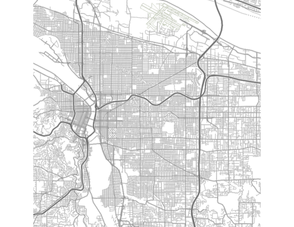
Portland, like many cities, has a mix of north/south and east/west aligned streets. However, it also has a non-trivial number of obliquely-oriented streets and parcels. This is especially the case in downtown Portland, east of the Williamette River and south of West Burnside Street. Given the concentration of calls for service in this area, it seemed likely that a non-standard alignment could be beneficial, especially for all calls for service. For this reason, grid angle of rotation was included as another parameter to be learned by the model, an idea first proposed by (Johnson et al., 2009).

Figure A5: Central Portland

Non-uniform land use coupled in Portland with the common practice of geocoding crime data to the street grid suggested that a fixed N/S oriented square tessellation could be sub-optimal (Rosser et al., 2016). However, contest rules required that shapes be polygons that could be tesselated without rotation. While squares were the simplest choice, the nature of the calls for service data geocoded to the street grid suggested that rectangles could be preferable. For this reason, we chose to leave the cell shape as a parameter to be optimized with each crime type and forecasting period potentially receiving its own optimized solution. Similarly, contest rules permitted a variety of different cell sizes and consistent with recent working demonstrating the sensitivity of forecast accuracy to cell size (Hart and Zandbergen, 2014), we left this as a parameter to be optimized. Subject to processing resource limitations, theoretically, any parameter could be optimized for forecasting accuracy.

The final hyperparameters we selected are shown in Table A1. Winning entries are highlighted in yellow.

Horizontal grid size (ft) Vertical grid size (ft) Coverage area Spatial lengthscale (ft) Temporal lengthscale (days) Rotation angle (radians) Number of random features $d$ l1 regularization l2 regularization KDE bandwidth (ft) Number of KDE lags KDE window (days) Crime Type Forecasting Period 478 710 10% 570 67.10 0.85 362 0 5e-5 274.70 9 39.62 ACFS 1m 618 473 16% 457.5 42.93 0.25 360 0 0 391.97 9 68.73 ACFS 1w 600 600 0% 250 60 0 250 0 1e-5 500 8 45 ACFS 2m 600 600 0% 250 28 0 250 0 5e-4 500 12 45 ACFS 2w 600 600 5% 500 90 0 20 1e-5 1e-4 500 6 90 ACFS 3m 250 250 95% 125 60 0 5 0 5e-5 250 12 15 burglary 1m 250 250 95% 750 7 0 20 0 0 250 6 10 burglary 1w 431 598 10% 1250 18.95 0 10 0 1e-4 342.42 10 3.50 burglary 2m 250 250 100% 125 70 0 5 0 1e-5 250 6 21 burglary 2w 689 484 15% 847.5 105.96 0.37 36 0 0 597.12 4 14.77 burglary 3m 600 600 15% 250 15 0.98 20 0 0 500 3 15 street 1m 600 600 10% 125 3.50 0 250 0 0 500 6 7 street 1w 600 600 10% 375 120 0.98 20 0 0 500 1 60 street 2m 600 600 5% 125 7 0.98 250 0 0 500 3 14 street 2w 600 600 0% 500 90 1.18 20 0 5e-4 500 3 45 street 3m 800 450 0% 125 150 0 5 0 5-e4 500 3 15 auto 1m 250 250 95% 500 49 0 5 0 0 250 6 10 auto 1w 600 600 80% 125 60 0 20 0 0 500 1 30 auto 2m 250 250 100% 750 14 0 5 0 0 250 3 21 auto 2w 600 600 0% 125 180 0 20 0 1e-5 500 3 45 auto 3m

Table A1: Final hyperparameters submitted to the competition. Yellow are winning rows for the PEI metric. We also won for the PAI metric for burglary 1 week and 2 weeks. Coverage area is a percentage of the range of areas allowed in the competition: 0% is the minimum (0.25 sq miles) and 100% is the maximum (0.75 sq miles). ACFS = all calls for service, street = street crime, auto = theft of auto.

References

- Adams, Murray and MacKay (2009) {binproceedings}[author] \bauthor\bsnmAdams, \bfnmRyan Prescott\binitsR. P., \bauthor\bsnmMurray, \bfnmIain\binitsI. and \bauthor\bsnmMacKay, \bfnmDavid JC\binitsD. J. (\byear2009). \btitleTractable nonparametric Bayesian inference in Poisson processes with Gaussian process intensities. In \bbooktitleProceedings of the 26th Annual International Conference on Machine Learning \bpages9–16. \bpublisherACM. \endbibitem
- Adepeju, Rosser and Cheng (2016) {barticle}[author] \bauthor\bsnmAdepeju, \bfnmMonsuru\binitsM., \bauthor\bsnmRosser, \bfnmGabriel\binitsG. and \bauthor\bsnmCheng, \bfnmTao\binitsT. (\byear2016). \btitleNovel evaluation metrics for sparse spatio-temporal point process hotspot predictions - a crime case study. \bjournalInternational Journal of Geographical Information Science \bvolume30 \bpages2133–2154. \bdoi10.1080/13658816.2016.1159684 \endbibitem
- Berk et al. (2018) {barticle}[author] \bauthor\bsnmBerk, \bfnmRichard\binitsR., \bauthor\bsnmHeidari, \bfnmHoda\binitsH., \bauthor\bsnmJabbari, \bfnmShahin\binitsS., \bauthor\bsnmKearns, \bfnmMichael\binitsM. and \bauthor\bsnmRoth, \bfnmAaron\binitsA. (\byear2018). \btitleFairness in criminal justice risk assessments: The state of the art. \bjournalSociological Methods & Research \bpages0049124118782533. \endbibitem
- Bhatt et al. (2017) {barticle}[author] \bauthor\bsnmBhatt, \bfnmSamir\binitsS., \bauthor\bsnmCameron, \bfnmEwan\binitsE., \bauthor\bsnmFlaxman, \bfnmSeth R\binitsS. R., \bauthor\bsnmWeiss, \bfnmDaniel J\binitsD. J., \bauthor\bsnmSmith, \bfnmDavid L\binitsD. L. and \bauthor\bsnmGething, \bfnmPeter W\binitsP. W. (\byear2017). \btitleImproved prediction accuracy for disease risk mapping using Gaussian process stacked generalization. \bjournalJournal of The Royal Society Interface \bvolume14 \bpages20170520. \endbibitem
- Brix and Diggle (2001) {barticle}[author] \bauthor\bsnmBrix, \bfnmAnders\binitsA. and \bauthor\bsnmDiggle, \bfnmPeter J\binitsP. J. (\byear2001). \btitleSpatiotemporal prediction for log-Gaussian Cox processes. \bjournalJournal of the Royal Statistical Society: Series B (Statistical Methodology) \bvolume63 \bpages823–841. \endbibitem
- Caplan, Kennedy and Miller (2011) {barticle}[author] \bauthor\bsnmCaplan, \bfnmJoel M.\binitsJ. M., \bauthor\bsnmKennedy, \bfnmLeslie W.\binitsL. W. and \bauthor\bsnmMiller, \bfnmJoel\binitsJ. (\byear2011). \btitleRisk Terrain Modeling: Brokering Criminological Theory and GIS Methods for Crime Forecasting. \bjournalJustice Quarterly \bvolume28 \bpages360–381. \bdoi10.1080/07418825.2010.486037 \endbibitem
- Carstensen et al. (2010) {barticle}[author] \bauthor\bsnmCarstensen, \bfnmLisbeth\binitsL., \bauthor\bsnmSandelin, \bfnmAlbin\binitsA., \bauthor\bsnmWinther, \bfnmOle\binitsO. and \bauthor\bsnmHansen, \bfnmNiels R.\binitsN. R. (\byear2010). \btitleMultivariate Hawkes process models of the occurrence of regulatory elements. \bjournalBMC Bioinformatics \bvolume11 \bpages456. \bdoi10.1186/1471-2105-11-456 \endbibitem
- Chainey (2013) {barticle}[author] \bauthor\bsnmChainey, \bfnmS. P.\binitsS. P. (\byear2013). \btitleExamining the influence of cell size and bandwidth size on kernel density estimation crime hotspot maps for predicting spatial patterns of crime. \bjournalBulletin of the Geographical Society of Liege \bvolume60 \bpages7–19. \endbibitem
- Chainey and Ratcliffe (2005) {bbook}[author] \bauthor\bsnmChainey, \bfnmSpencer\binitsS. and \bauthor\bsnmRatcliffe, \bfnmJerry\binitsJ. (\byear2005). \btitleGIS and crime mapping. \bpublisherJohn Wiley & Sons. \endbibitem
- Chainey, Tompson and Uhlig (2008a) {barticle}[author] \bauthor\bsnmChainey, \bfnmSpencer\binitsS., \bauthor\bsnmTompson, \bfnmLisa\binitsL. and \bauthor\bsnmUhlig, \bfnmSebastian\binitsS. (\byear2008a). \btitleThe Utility of Hotspot Mapping for Predicting Spatial Patterns of Crime. \bjournalSecurity Journal \bvolume21 \bpages4–28. \bdoi10.1057/palgrave.sj.8350066 \endbibitem
- Chainey, Tompson and Uhlig (2008b) {barticle}[author] \bauthor\bsnmChainey, \bfnmSpencer\binitsS., \bauthor\bsnmTompson, \bfnmLisa\binitsL. and \bauthor\bsnmUhlig, \bfnmSebastian\binitsS. (\byear2008b). \btitleResponse to Levine. \bjournalSecurity Journal \bvolume21 \bpages303–306. \bdoi10.1057/sj.2008.7 \endbibitem
- Choi and Schervish (2007) {barticle}[author] \bauthor\bsnmChoi, \bfnmTaeryon\binitsT. and \bauthor\bsnmSchervish, \bfnmMark J\binitsM. J. (\byear2007). \btitleOn posterior consistency in nonparametric regression problems. \bjournalJournal of Multivariate Analysis \bvolume98 \bpages1969–1987. \endbibitem
- Cohen, Gorr and Olligschlaeger (2007) {barticle}[author] \bauthor\bsnmCohen, \bfnmJacqueline\binitsJ., \bauthor\bsnmGorr, \bfnmWilpen L\binitsW. L. and \bauthor\bsnmOlligschlaeger, \bfnmAndreas M\binitsA. M. (\byear2007). \btitleLeading indicators and spatial interactions: A crime-forecasting model for proactive police deployment. \bjournalGeographical Analysis \bvolume39 \bpages105–127. \endbibitem
- Corbett-Davies et al. (2017) {binproceedings}[author] \bauthor\bsnmCorbett-Davies, \bfnmSam\binitsS., \bauthor\bsnmPierson, \bfnmEmma\binitsE., \bauthor\bsnmFeller, \bfnmAvi\binitsA., \bauthor\bsnmGoel, \bfnmSharad\binitsS. and \bauthor\bsnmHuq, \bfnmAziz\binitsA. (\byear2017). \btitleAlgorithmic decision making and the cost of fairness. In \bbooktitleProceedings of the 23rd ACM SIGKDD International Conference on Knowledge Discovery and Data Mining \bpages797–806. \bpublisherACM. \endbibitem
- Cressie and Wikle (2011) {bbook}[author] \bauthor\bsnmCressie, \bfnmN.\binitsN. and \bauthor\bsnmWikle, \bfnmC. K.\binitsC. K. (\byear2011). \btitleStatistics for spatio-temporal data \bvolume465. \bpublisherWiley. \endbibitem
- Cunningham, Shenoy and Sahani (2008) {binproceedings}[author] \bauthor\bsnmCunningham, \bfnmJohn P\binitsJ. P., \bauthor\bsnmShenoy, \bfnmKrishna V\binitsK. V. and \bauthor\bsnmSahani, \bfnmManeesh\binitsM. (\byear2008). \btitleFast Gaussian process methods for point process intensity estimation. In \bbooktitleProceedings of the 25th international conference on Machine learning \bpages192–199. \bpublisherACM. \endbibitem
- Diggle et al. (2013) {barticle}[author] \bauthor\bsnmDiggle, \bfnmPeter J\binitsP. J., \bauthor\bsnmMoraga, \bfnmPaula\binitsP., \bauthor\bsnmRowlingson, \bfnmBarry\binitsB., \bauthor\bsnmTaylor, \bfnmBenjamin M\binitsB. M. \betalet al. (\byear2013). \btitleSpatial and spatio-temporal Log-Gaussian Cox processes: extending the geostatistical paradigm. \bjournalStatistical Science \bvolume28 \bpages542–563. \endbibitem
- Dressel and Farid (2018) {barticle}[author] \bauthor\bsnmDressel, \bfnmJulia\binitsJ. and \bauthor\bsnmFarid, \bfnmHany\binitsH. (\byear2018). \btitleThe accuracy, fairness, and limits of predicting recidivism. \bjournalScience Advances \bvolume4. \bdoi10.1126/sciadv.aao5580 \endbibitem
- Fernandez and Teh (2016) {bunpublished}[author] \bauthor\bsnmFernandez, \bfnmT.\binitsT. and \bauthor\bsnmTeh, \bfnmY. W.\binitsY. W. (\byear2016). \btitlePosterior Consistency for a Non-parametric Survival Model under a Gaussian Process Prior. \bnotearXiv e-prints: 1611.02335. \endbibitem
- Flaxman (2014) {barticle}[author] \bauthor\bsnmFlaxman, \bfnmSeth R\binitsS. R. (\byear2014). \btitleA General Approach to Prediction and Forecasting Crime Rates with Gaussian Processes. \bjournalHeinz College Technical Report. \endbibitem
- Flaxman et al. (2015) {binproceedings}[author] \bauthor\bsnmFlaxman, \bfnmSeth\binitsS., \bauthor\bsnmWilson, \bfnmAndrew\binitsA., \bauthor\bsnmNeill, \bfnmDaniel\binitsD., \bauthor\bsnmNickisch, \bfnmHannes\binitsH. and \bauthor\bsnmSmola, \bfnmAlex\binitsA. (\byear2015). \btitleFast Kronecker inference in Gaussian processes with non-Gaussian likelihoods. In \bbooktitleInternational Conference on Machine Learning \bpages607–616. \endbibitem
- Friedman, Hastie and Tibshirani (2010) {barticle}[author] \bauthor\bsnmFriedman, \bfnmJerome\binitsJ., \bauthor\bsnmHastie, \bfnmTrevor\binitsT. and \bauthor\bsnmTibshirani, \bfnmRob\binitsR. (\byear2010). \btitleRegularization paths for generalized linear models via coordinate descent. \bjournalJournal of statistical software \bvolume33 \bpages1. \endbibitem
- Gerber (2014) {barticle}[author] \bauthor\bsnmGerber, \bfnmMatthew S\binitsM. S. (\byear2014). \btitlePredicting crime using Twitter and kernel density estimation. \bjournalDecision Support Systems \bvolume61 \bpages115–125. \endbibitem
- Gerhard, Deger and Truccolo (2017) {barticle}[author] \bauthor\bsnmGerhard, \bfnmFelipe\binitsF., \bauthor\bsnmDeger, \bfnmMoritz\binitsM. and \bauthor\bsnmTruccolo, \bfnmWilson\binitsW. (\byear2017). \btitleOn the stability and dynamics of stochastic spiking neuron models: Nonlinear Hawkes process and point process GLMs. \bjournalPLoS computational biology \bvolume13 \bpagese1005390. \endbibitem
- Gorr (2009) {barticle}[author] \bauthor\bsnmGorr, \bfnmWilpen L\binitsW. L. (\byear2009). \btitleForecast accuracy measures for exception reporting using receiver operating characteristic curves. \bjournalInternational Journal of Forecasting \bvolume25 \bpages48–61. \endbibitem
- Gorr and Lee (2015) {barticle}[author] \bauthor\bsnmGorr, \bfnmWilpen L.\binitsW. L. and \bauthor\bsnmLee, \bfnmYongJei\binitsY. (\byear2015). \btitleEarly Warning System for Temporary Crime Hot Spots. \bjournalJournal of Quantitative Criminology \bvolume31 \bpages25–47. \bdoi10.1007/s10940-014-9223-8 \endbibitem
- Gorr, Olligschlaeger and Thompson (2003) {barticle}[author] \bauthor\bsnmGorr, \bfnmWilpen\binitsW., \bauthor\bsnmOlligschlaeger, \bfnmAndreas\binitsA. and \bauthor\bsnmThompson, \bfnmYvonne\binitsY. (\byear2003). \btitleShort-term forecasting of crime. \bjournalInternational Journal of Forecasting \bvolume19 \bpages579–594. \bdoi10.1016/S0169-2070(03)00092-X \endbibitem
- Groff and Taniguchi (2019) {barticle}[author] \bauthor\bsnmGroff, \bfnmElizabeth\binitsE. and \bauthor\bsnmTaniguchi, \bfnmTravis\binitsT. (\byear2019). \btitleUsing citizen notification to interrupt near-repeat residential burglary patterns: the micro-level near-repeat experiment. \bjournalJournal of Experimental Criminology \bpages1–35. \endbibitem
- Guttorp and Gneiting (2005) {barticle}[author] \bauthor\bsnmGuttorp, \bfnmP\binitsP. and \bauthor\bsnmGneiting, \bfnmT\binitsT. (\byear2005). \btitleOn the Whittle-Matérn correlation family. \bjournalNational Research Center for Statistics and the Environment-Technical Report Series, Seattle, Washington. \endbibitem
- Hart and Zandbergen (2014) {barticle}[author] \bauthor\bsnmHart, \bfnmTimothy\binitsT. and \bauthor\bsnmZandbergen, \bfnmPaul\binitsP. (\byear2014). \btitleKernel density estimation and hotspot mapping: Examining the influence of interpolation method, grid cell size, and bandwidth on crime forecasting. \bjournalPolicing: An International Journal of Police Strategies & Management \bvolume37 \bpages305–323. \bdoi10.1108/PIJPSM-04-2013-0039 \endbibitem
- Heaton et al. (2018) {barticle}[author] \bauthor\bsnmHeaton, \bfnmMatthew J\binitsM. J., \bauthor\bsnmDatta, \bfnmAbhirup\binitsA., \bauthor\bsnmFinley, \bfnmAndrew O\binitsA. O., \bauthor\bsnmFurrer, \bfnmReinhard\binitsR., \bauthor\bsnmGuinness, \bfnmJoseph\binitsJ., \bauthor\bsnmGuhaniyogi, \bfnmRajarshi\binitsR., \bauthor\bsnmGerber, \bfnmFlorian\binitsF., \bauthor\bsnmGramacy, \bfnmRobert B\binitsR. B., \bauthor\bsnmHammerling, \bfnmDorit\binitsD., \bauthor\bsnmKatzfuss, \bfnmMatthias\binitsM. \betalet al. (\byear2018). \btitleA case study competition among methods for analyzing large spatial data. \bjournalJournal of Agricultural, Biological and Environmental Statistics \bpages1–28. \endbibitem
- Hennig, Osborne and Girolami (2015) {barticle}[author] \bauthor\bsnmHennig, \bfnmPhilipp\binitsP., \bauthor\bsnmOsborne, \bfnmMichael A.\binitsM. A. and \bauthor\bsnmGirolami, \bfnmMark\binitsM. (\byear2015). \btitleProbabilistic numerics and uncertainty in computations. \bjournalProceedings of the Royal Society of London A: Mathematical, Physical and Engineering Sciences \bvolume471. \endbibitem
- Hunt (2016) {bphdthesis}[author] \bauthor\bsnmHunt, \bfnmJoel M\binitsJ. M. (\byear2016). \btitleDo crime hot spots move? Exploring the effects of the modifiable areal unit problem and modifiable temporal unit problem on crime hot spot stability, \btypePhD thesis, \bpublisherAmerican University. \endbibitem
- Johnson et al. (2009) {bincollection}[author] \bauthor\bsnmJohnson, \bfnmShane D\binitsS. D., \bauthor\bsnmBowers, \bfnmKate J\binitsK. J., \bauthor\bsnmBirks, \bfnmD. J.\binitsD. J. and \bauthor\bsnmPease, \bfnmKen\binitsK. (\byear2009). \btitlePredictive mapping of crime by ProMap: accuracy, units of analysis, and the environmental backcloth. In \bbooktitlePutting Crime in its Place (\beditor\bfnmDavid\binitsD. \bsnmWeisburd, \beditor\bfnmWim\binitsW. \bsnmBernasco and \beditor\bfnmGerben\binitsG. \bsnmBruinsma, eds.) \bpages165–192. \bpublisherSpringer, \baddressDordrecht. \endbibitem
- Kang and Kang (2017) {barticle}[author] \bauthor\bsnmKang, \bfnmHyeon-Woo\binitsH.-W. and \bauthor\bsnmKang, \bfnmHang-Bong\binitsH.-B. (\byear2017). \btitlePrediction of crime occurrence from multi-modal data using deep learning. \bjournalPLOS ONE \bvolume12 \bpagese0176244. \bdoi10.1371/journal.pone.0176244 \endbibitem
- Levine (2004) {btechreport}[author] \bauthor\bsnmLevine, \bfnmNed\binitsN. (\byear2004). \btitleCrimeStat: a spatial statistics program for the analysis of crime incident locations, version 3.0. \btypeTechnical Report, \bpublisherNed Levine and Associates/National Institute of Justice, \baddressWashington, DC. \endbibitem
- Liu and Brown (2003) {barticle}[author] \bauthor\bsnmLiu, \bfnmHua\binitsH. and \bauthor\bsnmBrown, \bfnmDonald E.\binitsD. E. (\byear2003). \btitleCriminal incident prediction using a point-pattern-based density model. \bjournalInternational Journal of Forecasting \bvolume19 \bpages603–622. \bdoi10.1016/S0169-2070(03)00094-3 \endbibitem
- Lloyd et al. (2015) {binproceedings}[author] \bauthor\bsnmLloyd, \bfnmChris\binitsC., \bauthor\bsnmGunter, \bfnmTom\binitsT., \bauthor\bsnmOsborne, \bfnmMichael\binitsM. and \bauthor\bsnmRoberts, \bfnmStephen\binitsS. (\byear2015). \btitleVariational inference for Gaussian process modulated Poisson processes. In \bbooktitleInternational Conference on Machine Learning \bpages1814–1822. \endbibitem
- Loeffler and Flaxman (2018) {barticle}[author] \bauthor\bsnmLoeffler, \bfnmCharles\binitsC. and \bauthor\bsnmFlaxman, \bfnmSeth\binitsS. (\byear2018). \btitleIs gun violence contagious? A spatiotemporal test. \bjournalJournal of Quantitative Criminology \bvolume34 \bpages999–1017. \endbibitem
- Lum and Isaac (2016) {barticle}[author] \bauthor\bsnmLum, \bfnmKristian\binitsK. and \bauthor\bsnmIsaac, \bfnmWilliam\binitsW. (\byear2016). \btitleTo predict and serve? \bjournalSignificance \bvolume13 \bpages14–19. \endbibitem
- Makridakis, Spiliotis and Assimakopoulos (2018) {barticle}[author] \bauthor\bsnmMakridakis, \bfnmSpyros\binitsS., \bauthor\bsnmSpiliotis, \bfnmEvangelos\binitsE. and \bauthor\bsnmAssimakopoulos, \bfnmVassilios\binitsV. (\byear2018). \btitleStatistical and Machine Learning forecasting methods: Concerns and ways forward. \bjournalPloS one \bvolume13 \bpagese0194889. \endbibitem
- May et al. (2019) {barticle}[author] \bauthor\bsnmMay, \bfnmAvner\binitsA., \bauthor\bsnmGarakani, \bfnmAlireza Bagheri\binitsA. B., \bauthor\bsnmLu, \bfnmZhiyun\binitsZ., \bauthor\bsnmGuo, \bfnmDong\binitsD., \bauthor\bsnmLiu, \bfnmKuan\binitsK., \bauthor\bsnmBellet, \bfnmAurélien\binitsA., \bauthor\bsnmFan, \bfnmLinxi\binitsL., \bauthor\bsnmCollins, \bfnmMichael\binitsM., \bauthor\bsnmHsu, \bfnmDaniel\binitsD., \bauthor\bsnmKingsbury, \bfnmBrian\binitsB., \bauthor\bsnmPicheny, \bfnmMichael\binitsM. and \bauthor\bsnmSha, \bfnmFei\binitsF. (\byear2019). \btitleKernel Approximation Methods for Speech Recognition. \bjournalJournal of Machine Learning Research \bvolume20 \bpages1-36. \endbibitem
- Milton, Giorgi and Bhatt (2019) {barticle}[author] \bauthor\bsnmMilton, \bfnmPhilip\binitsP., \bauthor\bsnmGiorgi, \bfnmEmanuele\binitsE. and \bauthor\bsnmBhatt, \bfnmSamir\binitsS. (\byear2019). \btitleSpatial Analysis Made Easy with Linear Regression and Kernels. \bnotearXiv e-prints: 1902.08679. \endbibitem
- Mitchell, Potash and Barocas (2018) {barticle}[author] \bauthor\bsnmMitchell, \bfnmShira\binitsS., \bauthor\bsnmPotash, \bfnmEric\binitsE. and \bauthor\bsnmBarocas, \bfnmSolon\binitsS. (\byear2018). \btitlePrediction-based decisions and fairness: A catalogue of choices, assumptions, and definitions. \bjournalarXiv preprint arXiv:1811.07867. \endbibitem
- Mohler (2014) {barticle}[author] \bauthor\bsnmMohler, \bfnmGeorge\binitsG. (\byear2014). \btitleMarked point process hotspot maps for homicide and gun crime prediction in Chicago. \bjournalInternational Journal of Forecasting \bvolume30 \bpages491–497. \endbibitem
- Mohler et al. (2013) {barticle}[author] \bauthor\bsnmMohler, \bfnmGeorge\binitsG. \betalet al. (\byear2013). \btitleModeling and estimation of multi-source clustering in crime and security data. \bjournalThe Annals of Applied Statistics \bvolume7 \bpages1525–1539. \endbibitem
- Mohler and Porter (2018) {barticle}[author] \bauthor\bsnmMohler, \bfnmGeorge\binitsG. and \bauthor\bsnmPorter, \bfnmMichael D\binitsM. D. (\byear2018). \btitleRotational grid, PAI-maximizing crime forecasts. \bjournalStatistical Analysis and Data Mining: The ASA Data Science Journal \bvolume11 \bpages227–236. \endbibitem
- Mohler et al. (2011) {barticle}[author] \bauthor\bsnmMohler, \bfnmG. O.\binitsG. O., \bauthor\bsnmShort, \bfnmM. B.\binitsM. B., \bauthor\bsnmBrantingham, \bfnmP. J.\binitsP. J., \bauthor\bsnmSchoenberg, \bfnmF. P.\binitsF. P. and \bauthor\bsnmTita, \bfnmG. E.\binitsG. E. (\byear2011). \btitleSelf-Exciting Point Process Modeling of Crime. \bjournalJournal of the American Statistical Association \bvolume106 \bpages100–108. \bdoi10.1198/jasa.2011.ap09546 \endbibitem
- Mohler et al. (2015) {barticle}[author] \bauthor\bsnmMohler, \bfnmG. O.\binitsG. O., \bauthor\bsnmShort, \bfnmM. B.\binitsM. B., \bauthor\bsnmMalinowski, \bfnmSean\binitsS., \bauthor\bsnmJohnson, \bfnmMark\binitsM., \bauthor\bsnmTita, \bfnmG. E.\binitsG. E., \bauthor\bsnmBertozzi, \bfnmAndrea L.\binitsA. L. and \bauthor\bsnmBrantingham, \bfnmP. J.\binitsP. J. (\byear2015). \btitleRandomized Controlled Field Trials of Predictive Policing. \bjournalJournal of the American Statistical Association \bvolume110 \bpages1399-1411. \endbibitem
- Møller and Rasmussen (2005) {barticle}[author] \bauthor\bsnmMøller, \bfnmJesper\binitsJ. and \bauthor\bsnmRasmussen, \bfnmJakob G\binitsJ. G. (\byear2005). \btitlePerfect simulation of Hawkes processes. \bjournalAdvances in applied probability \bvolume37 \bpages629–646. \endbibitem
- Møller, Syversveen and Waagepetersen (1998) {barticle}[author] \bauthor\bsnmMøller, \bfnmJesper\binitsJ., \bauthor\bsnmSyversveen, \bfnmAnne Randi\binitsA. R. and \bauthor\bsnmWaagepetersen, \bfnmRasmus Plenge\binitsR. P. (\byear1998). \btitleLog gaussian cox processes. \bjournalScandinavian journal of statistics \bvolume25 \bpages451–482. \endbibitem
- National Institute of Justice (2017) {bmisc}[author] \bauthor\bsnmNational Institute of Justice (\byear2017). \btitleReal-Time Crime Forecasting Challenge. \bnotehttp://www.nij.gov/funding/Pages/fy16-crime-forecasting-challenge.aspx. \endbibitem
- Ogata (1988) {barticle}[author] \bauthor\bsnmOgata, \bfnmYosihiko\binitsY. (\byear1988). \btitleStatistical models for earthquake occurrences and residual analysis for point processes. \bjournalJournal of the American Statistical association \bvolume83 \bpages9–27. \endbibitem
- O’Hagan (1992) {barticle}[author] \bauthor\bsnmO’Hagan, \bfnmAnthony\binitsA. (\byear1992). \btitleSome Bayesian numerical analysis. \bjournalBayesian Statistics \bvolume4 \bpages4–2. \endbibitem
- Pease et al. (1998) {bbook}[author] \bauthor\bsnmPease, \bfnmKenneth\binitsK. \betalet al. (\byear1998). \btitleRepeat victimisation: Taking stock \bvolume90. \bpublisherHome Office Police Research Group London. \endbibitem
- Perry et al. (2013) {btechreport}[author] \bauthor\bsnmPerry, \bfnmWalter L.\binitsW. L., \bauthor\bsnmMcInnis, \bfnmBrian\binitsB., \bauthor\bsnmPrice, \bfnmCarter C.\binitsC. C., \bauthor\bsnmSmith, \bfnmSusan C.\binitsS. C. and \bauthor\bsnmHollywood, \bfnmJohn S.\binitsJ. S. (\byear2013). \btitlePredictive Policing: The Role of Crime Forecasting in Law Enforcement Operations \btypeTechnical Report, \bpublisherRAND Corporation, \baddressSanta Monica. \endbibitem
- Porter and Reich (2012) {barticle}[author] \bauthor\bsnmPorter, \bfnmMichael D.\binitsM. D. and \bauthor\bsnmReich, \bfnmBrian J.\binitsB. J. (\byear2012). \btitleEvaluating temporally weighted kernel density methods for predicting the next event location in a series. \bjournalAnnals of GIS \bvolume18 \bpages225–240. \bdoi10.1080/19475683.2012.691904 \endbibitem
- Rahimi and Recht (2007) {binproceedings}[author] \bauthor\bsnmRahimi, \bfnmAli\binitsA. and \bauthor\bsnmRecht, \bfnmBenjamin\binitsB. (\byear2007). \btitleRandom features for large-scale kernel machines. In \bbooktitleAdvances in neural information processing systems \bpages1177–1184. \endbibitem
- Rahimi and Recht (2008) {binproceedings}[author] \bauthor\bsnmRahimi, \bfnmAli\binitsA. and \bauthor\bsnmRecht, \bfnmBenjamin\binitsB. (\byear2008). \btitleWeighted sums of random kitchen sinks: Replacing minimization with randomization in learning. In \bbooktitleAdvances in neural information processing systems \bpages1313–1320. \endbibitem
- Rasmussen and Williams (2006) {bbook}[author] \bauthor\bsnmRasmussen, \bfnmCarl Edward\binitsC. E. and \bauthor\bsnmWilliams, \bfnmChristopher KI\binitsC. K. (\byear2006). \btitleGaussian Processes for Machine Learning. \bpublisherMIT Press. \endbibitem
- Rodrigues and Diggle (2012) {barticle}[author] \bauthor\bsnmRodrigues, \bfnmAlexandre\binitsA. and \bauthor\bsnmDiggle, \bfnmPeter J.\binitsP. J. (\byear2012). \btitleBayesian Estimation and Prediction for Inhomogeneous Spatiotemporal Log-Gaussian Cox Processes Using Low-Rank Models, With Application to Criminal Surveillance. \bjournalJournal of the American Statistical Association \bvolume107 \bpages93–101. \endbibitem
- Rosser and Cheng (2016) {barticle}[author] \bauthor\bsnmRosser, \bfnmGabriel\binitsG. and \bauthor\bsnmCheng, \bfnmTao\binitsT. (\byear2016). \btitleImproving the Robustness and Accuracy of Crime Prediction with the Self-Exciting Point Process Through Isotropic Triggering. \bjournalApplied Spatial Analysis and Policy \bpages1–21. \endbibitem
- Rosser et al. (2016) {barticle}[author] \bauthor\bsnmRosser, \bfnmGabriel\binitsG., \bauthor\bsnmDavies, \bfnmToby\binitsT., \bauthor\bsnmBowers, \bfnmKate J.\binitsK. J., \bauthor\bsnmJohnson, \bfnmShane D.\binitsS. D. and \bauthor\bsnmCheng, \bfnmTao\binitsT. (\byear2016). \btitlePredictive Crime Mapping: Arbitrary Grids or Street Networks? \bjournalJournal of Quantitative Criminology \bpages1–26. \bdoi10.1007/s10940-016-9321-x \endbibitem
- Rudin and Ustun (2018) {barticle}[author] \bauthor\bsnmRudin, \bfnmCynthia\binitsC. and \bauthor\bsnmUstun, \bfnmBerk\binitsB. (\byear2018). \btitleOptimized scoring systems: toward trust in machine learning for healthcare and criminal justice. \bjournalInterfaces \bvolume48 \bpages449–466. \endbibitem
- Schölkopf and Smola (2002) {bbook}[author] \bauthor\bsnmSchölkopf, \bfnmBernhard\binitsB. and \bauthor\bsnmSmola, \bfnmAlexander J\binitsA. J. (\byear2002). \btitleLearning with kernels: support vector machines, regularization, optimization and beyond. \bpublisherthe MIT Press. \endbibitem
- Schutt (1922) {barticle}[author] \bauthor\bsnmSchutt, \bfnmHarold G.\binitsH. G. (\byear1922). \btitleAdvanced police methods in Berkeley. \bjournalNational Municipal Review \bvolume11 \bpages80–85. \bdoi10.1002/ncr.4110110308 \endbibitem
- Shirota et al. (2017) {barticle}[author] \bauthor\bsnmShirota, \bfnmShinichiro\binitsS., \bauthor\bsnmGelfand, \bfnmAlan E\binitsA. E. \betalet al. (\byear2017). \btitleSpace and circular time log Gaussian Cox processes with application to crime event data. \bjournalThe Annals of Applied Statistics \bvolume11 \bpages481–503. \endbibitem
- Snoek, Larochelle and Adams (2012) {binproceedings}[author] \bauthor\bsnmSnoek, \bfnmJasper\binitsJ., \bauthor\bsnmLarochelle, \bfnmHugo\binitsH. and \bauthor\bsnmAdams, \bfnmRyan P\binitsR. P. (\byear2012). \btitlePractical bayesian optimization of machine learning algorithms. In \bbooktitleAdvances in neural information processing systems \bpages2951–2959. \endbibitem
- Sriperumbudur, Fukumizu and Lanckriet (2011) {barticle}[author] \bauthor\bsnmSriperumbudur, \bfnmBharath K\binitsB. K., \bauthor\bsnmFukumizu, \bfnmKenji\binitsK. and \bauthor\bsnmLanckriet, \bfnmGert RG\binitsG. R. (\byear2011). \btitleUniversality, characteristic kernels and RKHS embedding of measures. \bjournalJournal of Machine Learning Research \bvolume12 \bpages2389–2410. \endbibitem
- Stein (1999) {bbook}[author] \bauthor\bsnmStein, \bfnmMichael L\binitsM. L. (\byear1999). \btitleInterpolation of Spatial Data: Some Theory for Kriging. \bpublisherSpringer Science & Business Media. \endbibitem
- Sun, Li and Genton (2012) {bincollection}[author] \bauthor\bsnmSun, \bfnmYing\binitsY., \bauthor\bsnmLi, \bfnmBo\binitsB. and \bauthor\bsnmGenton, \bfnmMarc G\binitsM. G. (\byear2012). \btitleGeostatistics for large datasets. In \bbooktitleAdvances and challenges in space-time modelling of natural events \bpages55–77. \bpublisherSpringer. \endbibitem
- Taddy (2010) {barticle}[author] \bauthor\bsnmTaddy, \bfnmMatthew A.\binitsM. A. (\byear2010). \btitleAutoregressive Mixture Models for Dynamic Spatial Poisson Processes: Application to Tracking Intensity of Violent Crime. \bjournalJournal of the American Statistical Association \bvolume105 \bpages1403–1417. \bdoi10.1198/jasa.2010.ap09655 \endbibitem
- Teh and Rao (2011) {binproceedings}[author] \bauthor\bsnmTeh, \bfnmYee W\binitsY. W. and \bauthor\bsnmRao, \bfnmVinayak\binitsV. (\byear2011). \btitleGaussian process modulated renewal processes. In \bbooktitleAdvances in Neural Information Processing Systems \bpages2474–2482. \endbibitem
- Wang, Gerber and Brown (2012) {bincollection}[author] \bauthor\bsnmWang, \bfnmXiaofeng\binitsX., \bauthor\bsnmGerber, \bfnmMatthew S.\binitsM. S. and \bauthor\bsnmBrown, \bfnmDonald E.\binitsD. E. (\byear2012). \btitleAutomatic Crime Prediction Using Events Extracted from Twitter Posts. In \bbooktitleSocial Computing Behavioral - Cultural Modeling and Prediction \bpages231–238. \bpublisherSpringer Berlin Heidelberg. \endbibitem
- Weinberger et al. (2009) {binproceedings}[author] \bauthor\bsnmWeinberger, \bfnmKilian\binitsK., \bauthor\bsnmDasgupta, \bfnmAnirban\binitsA., \bauthor\bsnmLangford, \bfnmJohn\binitsJ., \bauthor\bsnmSmola, \bfnmAlex\binitsA. and \bauthor\bsnmAttenberg, \bfnmJosh\binitsJ. (\byear2009). \btitleFeature Hashing for Large Scale Multitask Learning. In \bbooktitleProceedings of the 26th Annual International Conference on Machine Learning. \bseriesICML ’09 \bpages1113–1120. \bpublisherACM, \baddressNew York, NY, USA. \bdoi10.1145/1553374.1553516 \endbibitem
- Zhu (2013) {barticle}[author] \bauthor\bsnmZhu, \bfnmLingjiong\binitsL. (\byear2013). \btitleCentral limit theorem for nonlinear Hawkes processes. \bjournalJournal of Applied Probability \bvolume50 \bpages760–771. \endbibitem
- Zou and Hastie (2005) {barticle}[author] \bauthor\bsnmZou, \bfnmHui\binitsH. and \bauthor\bsnmHastie, \bfnmTrevor\binitsT. (\byear2005). \btitleRegularization and variable selection via the elastic net. \bjournalJournal of the Royal Statistical Society: Series B (Statistical Methodology) \bvolume67 \bpages301–320. \endbibitem