Analyzing Mobility-Traffic Correlations in Large WLAN Traces: Flutes vs. Cellos

Abstract

Two major factors affecting mobile network performance are mobility and traffic patterns. Simulations and analytical-based performance evaluations rely on models to approximate factors affecting the network. Hence, the understanding of mobility and traffic is imperative to the effective evaluation and efficient design of future mobile networks. Current models target either mobility or traffic, but do not capture their interplay. Many trace-based mobility models have largely used pre-smartphone datasets (e.g., AP-logs), or much coarser granularity (e.g., cell-towers) traces. This raises questions regarding the relevance of existing models, and motivates our study to revisit this area. In this study, we conduct a multi-dimensional analysis, to quantitatively characterize mobility and traffic spatio-temporal patterns, for laptops and smartphones, leading to a detailed integrated mobility-traffic analysis. Our study is data-driven, as we collect and mine capacious datasets (with 30TB, 300k devices) that capture all of these dimensions. The investigation is performed using our systematic (FLAMeS) framework. Overall, dozens of mobility and traffic features have been analyzed. The insights and lessons learnt serve as guidelines and a first step towards future integrated mobility-traffic models. In addition, our work acts as a stepping-stone towards a richer, more-realistic suite of mobile test scenarios and benchmarks.

I Introduction

Human mobility has been studied extensively and many models have been derived. The spectrum ranges from simple synthetic mobility models to complex trace-based models, capturing different properties with varying degrees of accuracy [1, 2]. Similarly, network traffic has been studied increasingly for wireless networks: for rather stationary users (as in WLANs) (e.g., [3, 4]) and potentially mobile users as for cellular networks (e.g., [5, 6]). Such analyses range from metrics such as flow count, sizes, and traffic volume to service usage (e.g., visited web sites, backend services).

Both mobility and network usage, characterize different aspects of human behavior. In this sense, we have a mobility plane and a (network) traffic plane. In reality, these two planes are likely interdependent. Human mobility may be influenced by network activity; for example, a person slowing down to read incoming messages. Also, network activity may be influenced by mobility and location; stationary users may produce/consume more data than those walking, and people may use different services in different places [7].

In earlier studies, this interdependence has not been widely considered, and models for both mobility and network traffic planes have been developed and evaluated largely in isolation. For example, when evaluating mobile systems’ performance, traffic generation generally follows regular patterns, drawn from common simple distributions (e.g., exponential or uniform), while assuming neither transmission nor reception of data impacts mobility. Simply observing people walking while staring at (or reacting to) their smartphones suggests, however, that such interdependencies need to be captured properly. Understanding the mobility-traffic interplay is imperative to the effective evaluation and efficient design of future mobile algorithms ranging from user behavior prediction and caching, to network load estimation and resource allocation.

In this paper, we take a stab at understanding the interconnection of the mobility and traffic planes. To do this properly, we need to consider the nature of mobile devices people use: one class of devices is merely intended for stationary use, typically while the user is seated—this primarily holds for laptop computers, dubbed cellos. In contrast, another class—’on-the-go’ smartphones, which we refer to as flutes—lend themselves to truly mobile use. We focus our analysis on these two classes because they have been around long enough to have extensive datasets to build upon. We stipulate that the interconnection of the mobility and traffic is modulated by the device(s) a mobile user is carrying. Therefore, we follow two main lines of investigation: we develop a framework to differentiate between cellos and flutes, and study both the mobility and traffic patterns for each of those types.

Specifically, the main goal of this paper is to quantitatively investigate the following questions in-depth: (I) How different are mobility and traffic characteristics across device types, time and space? (II) What are the relationships between these characteristics? (III) Should new models be devised to capture these differences? And, if so, how?

To answer these questions, a multi-dimensional (comparative) analysis approach is adopted to investigate mobility and traffic spatio-temporal patterns for flutes and cellos. We drive our study with capacious datasets (30TB+) that capture all the above dimensions in a campus society, including over 300k devices (Sec. IV). A systematic Framework for Large-scale Analysis of Mobile Societies (FLAMeS) is devised for this study, that can also be used to analyze other multi-sourced data in future studies. Our main contributions include:

1. Integrated mobility-traffic analyses (Sec. VII): This study is the first to quantify the correlations of numerous features of mobility and traffic simultaneously. This can identify gaps in existing mobile networking models, and reopen the door for future impactful work in this area.

2. Flutes vs. Cellos analysis (Sec. V–VI): The device type classification presented here, is an important dimension to understand. This is particularly relevant as new generations of portable devices are introduced, that are different than laptops, traditionally considered in earlier studies.

3. Systematic multi-dimensional investigation framework (Sec. III): FLAMeS provides the scaffolding needed to process, in multiple dimensions, many features of large sets of measurements from wireless networks, including AP-logs and NetFlow traces. This systematic method can apply to other datasets in future studies.

II Related work

To characterize mobility and network usage, existing studies have covered various aspects, including human mobility, device variation, and dataset analysis.

Human Mobility: Given its importance in various research areas, human mobility has received significant attention. We refer the reader to [1, 2] for surveys of mobility modeling and analysis. For spatial-temporal patterns, [8] and [9] reveal the regularity and bounds for predicting human mobility using cellular logs. A recent study highlighted the importance of combining different datasets to study various features simultaneously [10]. Our observations are similar to [8, 9], which reaffirms the intrinsic properties of human mobility, despite differences in granularity and population across datasets. To advance the understanding of human mobility, we integrated different datasets to correlate mobility and network traffic.

Device Variation: Usage and traffic patterns of different device types have been studied from various perspectives ([11, 12, 13, 14, 15, 16]). However, those findings are based on classifications that rely on either MAC addresses or HTTP headers solely. The former is rather limited and the latter may have serious privacy implications and are often unavailable. In [17], authors use packet-level traces from 10 phones and application-level monitoring from 33 Android devices to analyze smartphone traffic. Although this allowed fine-grained measurements, the approach is invasive and limited in scalability, leading to small sample sizes and restricted conclusions. They also do not compare the traffic of smartphones with that of “stop-to-use” wireless devices (i.e. cellos) nor do they measure spatial metrics. The study in [18] analyzes 32k users on campus, and focuses on multi-device usage. It notes differences between laptops and smartphones in packets, content, and time of usage. That work targets device usage patterns and security, while we study mobility and wireless traffic correlations. In our method, the combination of MAC and NetFlow allowed us to classify majority of observed devices while preserving users’ privacy.

Dataset Analysis: A recent work on WLAN traces [19] revealed surprising patterns on increases of long-term mobility entropy by age, and the impact of academic majors on students’ long-term mobility entropy. The authors of [7] investigated correlations and characteristics of web domains accessed by users and their locations, based on NetFlow and DHCP logs from a university campus in 2004. They propose a simulation paradigm with data-driven parameters, producing realistic scenarios for simulations. However, that study uses data from pre-smartphone era and does not distinguish between device types. It also does not analyze the relation between mobility and traffic. On both WiFi and cellular networks, the authors of [20] performed an in-depth study on smartphone traffic, highlighting the benefits and limitations of using MPTCP. Distributions of flow inter-arrival time (IAT) and arrival rate at APs of “static” flows were analyzed (e.g., Exp, Weibull, Pareto, Lognormal) in [21]. Lognormal was found to best fit the flow sizes, while at small time scales (i.e. hourly), IAT was best described by Weibull but parameters vary from hour to hour. We analyze flows on a much larger scale, newer dataset including smartphones, and identify Lognormal distribution as the best fit for flow sizes, and beta as best for IAT, regardless of device type. The study in [22] analyzed ISP traces with 9600 cellular towers and 150K users in Shanghai, and mapped timed traffic patterns to urban regions. It provided insight into mobile traffic patterns across time, location and frequency. This work is complementary to ours, as we provide a much finer scope analyzing campus WLAN traces.

III Systematic multi-dimensional analysis

To methodically analyze statistical characteristics and correlations in multiple dimensions, we introduce the FLAMeS framework (Fig. 1). The main components include: I. Data collection and pre-processing, II. Flutes vs. cellos mobility and traffic analysis, and III. Integrated mobility-traffic analysis.

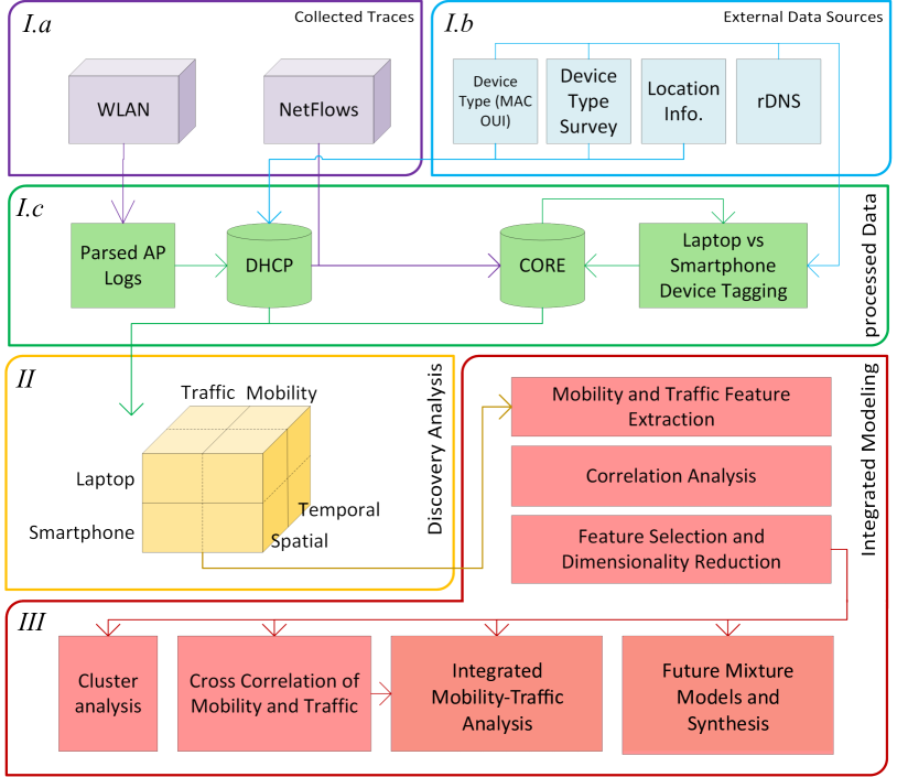
Figure 1: FLAMeS system overview.

The two main purposes of this work are to understand and quantify the gaps between flutes and cellos, and the interaction between the mobility and traffic dimensions. Individual mobility and traffic analyses for flutes and cellos are conducted in Sections V and VI, respectively, with detailed reporting for spatio-temporal features showing significant gaps. In Sec. VII, the most important mobility and traffic features are identified and their correlation quantified.

IV Experimental setup and datasets

We drive our framework with large-scale datasets from multiple sources, capturing the mobility and traffic features in different dimensions. In this section, we introduce the two data sets and their preprocessing, and present the device type classification into flutes and cellos.

The input datasets in this study are specifically chosen to capture: 1. location, mobility and network traffic information, 2. smartphone and laptop devices, 3. spatio-temporal features, and 4. scale in number of devices and records. The total size is $>$30TB, consisting of two main parts: WLAN Access Point (AP) logs, and Netflow records (details in Tables I, II).

IV-A WLAN AP logs

These logs are collected from 1760 APs in 138 buildings over 479 days on a university campus, and contain association and authentication events from 316k devices in 2011-2012. It contains over 555M records, with each record including the device’s MAC and assigned IP addresses, the associated AP and a timestamp. Locations of the APs are approximated by the building locations where they are installed, i.e., (longitude, latitude) of Google Maps API. To validate this, we fetched 8000 mapped APs around the campus area from a crowd-sourced service, wigle.net. For the 130 matched APs in 42% of buildings (i.e., 58 bldgs), all were less than 200m from their mapped location; an error of less than 1.5% of the campus area. This is very reasonable for our study purposes.

IV-B NetFlow logs

Over 76 billion records of NetFlow traces were collected from the same network, over 25 days in April 2012. A flow is defined as a consecutive sequence of packets with the same transport protocol, source/destination IP and port number, as identified by the collecting gateway router. An example of major Netflow data fields is presented in Table II.

The NetFlow records are matched with the wireless associations (from the AP logs) using the dynamic MAC-to-IP address mapping from the DHCP logs. We refer to the result as CORE dataset (Table I). They are also augmented with location and website information using reverse DNS (rDNS).

TABLE I: Summary of datasets. B=billion.

	# Records		Traffic Vol. (TB)		# MAC
	DHCP	CORE	TCP	UDP	WLAN	CORE
Flutes	412.0 M	2.13 B	56.18	4.50	186.0 K	50.3 K
Cellos	101.0 M	4.20 B	73.85	12.90	93.2 K	27.1 K
Total	557.5 M	6.53 B	134.39	17.61	316.0 K	80.0 K

IV-C Device type classification

To classify devices into flutes and cellos, we utilize several observations and heuristics. To start, note that a device manufacturer (with OUI) can be identified based on the first 3 octets of the MAC address. Most manufacturers produce one type of device (either laptop or phone), but some produce both (e.g., Apple). In the latter case, OUI used for one device type is not used for another. We conducted a survey to help classify 30 MAC prefixes accurately. Using OUI and survey information, we identify and label 46% of the total devices (90k cellos and 56k flutes). Then, from the NetFlow logs of these labeled devices, we observe over 3k devices (92% of which are flutes) contacting admob.com; an ad platform serving mainly smartphones and tablets (i.e. flutes). This enables further classification of the remaining MAC addresses. Finally, we apply the following heuristic to the dataset: (1) obtain all OUIs (MAC prefix) that contacted admob.com; (2) if it is unlabeled, mark it as a flute. Overall, over 270k devices were labeled (180k as flutes), covering 86% of the devices in AP logs and 97% in NetFlow traces, a reasonable coverage for our purposes. Out of $\approx 80k$ devices in the NetFlow logs, $\approx 50$K are flutes and $\approx 27$K cellos.

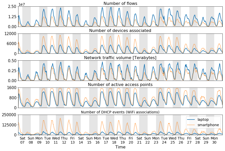
Figure 2: Time series for 25 days of combined AP-NetFlow Core traces

Fig. 2 shows the temporal plot for the combined traces over 25 days, after device classification. Throughout, the number of flows and total traffic volume is clearly higher for cellos, even with an overall higher number of flutes connected. Also note the device activities in a diurnal and weekly cycles, with the peaks occurring during weekdays, as expected. Wed, 25th, was the last day of classes, explaining the decline in network activity afterwards. This plot motivates our analyses for flutes vs cellos, over weekends vs weekdays, in this study.

TABLE II: NetFlow (top) and AP logs/DHCP (bottom) sample data

Start time Finish time Duration Source IP Destination IP Protocol Source port Destination port Packet count Flow size 1334332274.912 1334332276.576 1.664 173.194.37.7 10.15.225.126 TCP 80 60482 157 217708

User IP User MAC AP name AP MAC Lease begin time Lease end time 10.130.90.3 00:11:22:33:44:55 b422r143-win-1 00:1d:e5:8f:1b:30 1333238737 1333238741

V Mobility analysis

This section covers the temporal and spatial mobility analyses. For all metrics, unless otherwise noted, we investigate 479 days. A summary of studied metrics and their most significant statistical values are presented in Tab. III along with mean and median ratios for comparison. From that list, we further investigate in this section those metrics that show the most interesting or non-trivial differences between flutes and cellos.

TABLE III: General results for mobility. Upper values are for weekdays and lower ones for weekends (in red color). LJM: maximum jump [m]; DIA: diameter [m]; TJM: total trajectory length [m]; GYR: radius of gyration [m]; BLD: no. uniq. buildings; APC: access point count; PDT: time spent at preferred building [minutes]; DLT: total session time at each building.

	Flutes (F)			Cellos (C)			Ratio (C/F)
	$\mu$	mdn	$\sigma$	$\mu$	mdn	$\sigma$	$\mu$	mdn
LJM	435	296	813	178	1	624	0.409	0.003
	350	168	683	97	1	312	0.277	0.006
DIA	549	411	874	195	1	642	0.355	0.002
	425	179	739	107	1	338	0.252	0.006
TJM	1582	707	2336	378	1	1444	0.239	0.001
	1036	279	1793	252	1	1766	0.243	0.004
GYR	396	290	2725	321	191	3265	1.102	1.019
	330	248	1368	178	65.1	1800	1.247	1.4
BLD	5.4	3	5.6	1.8	1	2.1	0.811	0.659
	2.8	2	4.1	1.5	1	1.8	0.539	0.262
APC	11.8	6	13.3	3.7	2	4.8	0.333	0.333
	7.2	4	8.8	3	2	3.8	0.536	0.5
PDT	225	161	219	248	164	254	0.314	0.333
	223	135	272	278	189	292	0.417	0.5
DLT	316	235	302	316	217	305	1	0.92
	326	247	308	316	221	309	0.97	0.89

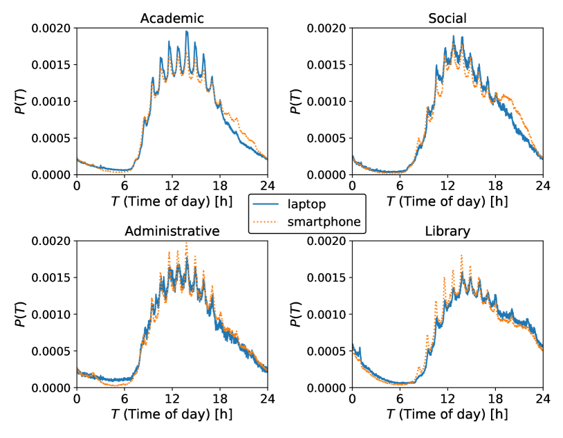
Figure 3: PDF Session start over time of the day.

V-A Session start probability

A session is defined as the period between WLAN associations. The distributions of session start times across the day for four building categories are depicted in Fig. 3. The start times of the Sessions match the periodic beginning of classes, but mainly in Academic buildings, where users move mostly at the start and end of classes. In these places, activity drops sharply for cellos at 5pm, with considerable flutes activity until 8pm. For Social and Library buildings, the probability of new sessions remains higher for a few more hours into the evening, and the times users tend to leave are more spread out. We do not make similar observation during weekends, which is expected when the day is, unlike weekdays, not governed by a class schedule. For most visitors, the session start distributions show a smooth shape and no significant differences between device types (omitted for brevity).

V-B Radius of gyration

This metric, $GYR$, captures the size of the geospatial dispersion of a device’s movements, denoted by $r_{g}$ and computed as $r_{g}=\frac{1}{N}\sum_{k=1}^{N}\left(\vec{r_{k}}-\vec{r_{s}}\right)^{2}$, where $\vec{r_{1}},...,\vec{r_{N}}$ are positional vectors of a device and $\vec{r_{s}}$ is its center of gravity.

Grouping devices by their $r_{g}$ after six months of observation, we look at its evolution since the first time they are observed. Unsurprisingly (cf. [8]), after an initial transient period of about one week, this value stabilizes even across different semesters (not shown).

We split the traces into weekdays and weekends, presenting the distributions in Fig. 4(a). For cellos, we notice a substantial reduction in their overall mobility whereas, for flutes, this difference is not so pronounced. This might be due to students having fewer activities on weekends, a tendency to study at a single building like a library, or just not carry their cellos; we will revisit this aspect in Sec. VII. Flutes, being “always-on” devices, are able to capture movements at pass-by locations, dining areas, and bus stops and thus are better suited to capture the fine-granular mobility of their users than cellos.

Despite the 8.1km² area of the campus (approximate radius of 1.42km), buildings with related fields of study (e.g. Fine Arts) are fairly clustered. Computing the distance between the k-nearest neighboring buildings, for $k=22$ and $k=9$ (average number of visited buildings for flutes and cellos) the median distances are 295m and 172m, respectively. Due to their focus on classes, attending students have limited area of activity on weekdays, which explains the observed radius of gyration.

We also evaluated: (1) diameter $DIA$, the longest distance between any pair of $\vec{r_{k}}$ points; (2) max jump $LJM$, the longest distance between a pair of consecutive $\vec{r_{k}}$ points; and (3) total trajectory length $TJM$, the sum of all trips made by a device. The distributions of these metrics are similar to Radius of Gyration and therefore not shown. Table III summarizes the most significant statistical values for these metrics.

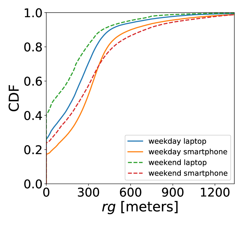
(a)

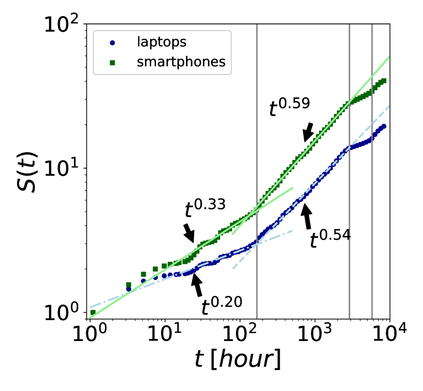
(b)

Figure 4: (a) Radius of gyration ($rg$ for the device types). (b) Visited locations $S\left(t\right)$. Vertical lines at 7, 120 and 240 days.

V-C Visitation preferences and interests

We count the number of unique buildings visited by a user, $BLD$, and define a preferred building as the location where a device has spent most of its time in a given day, measured in minutes and referred to as $PDT$. We approximate the latter by the formula $t_{b}=\sum_{k=1}^{N_{b}}S_{k}$, where $t_{b}$ is the time spent, $N_{b}$ the total number of sessions and $S_{1}...S_{N}$ the time duration of each session at a building $b$, here referred as $DLT$. Interestingly, cellos have slightly longer stays but both have medians around 2:40 hours. The similarity of the distributions, combined with a lower number of visited locations indicate that cellos are used mostly when users remain longer periods at places.

Fig. 4(b) highlights the differences between flutes and cellos on the required time $t$ to visit S(t) locations. After an initial exploration period of one week the rates of new visits change similarly for both device types, and new exploration rates show up at 120 and 240 days. These could be explained by the weekly schedules of the university as well as the usual length of a lecture term ($\approx 4$ months).

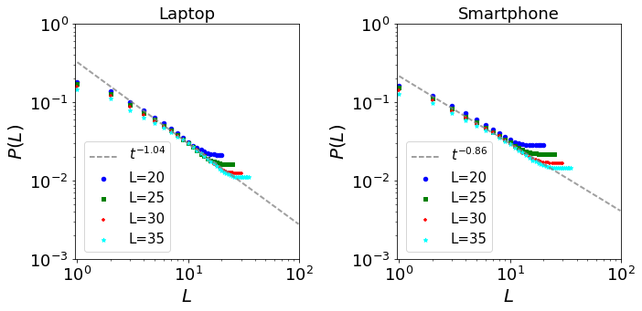
Figure 5: Zipf’s plot on $L$ visited access points.

We also consider the number of unique APs a device associates with, $APC$, which provides a finer spatial resolution than the building level. Furthermore, the probability of finding a device at its L-th most visited access point is shown in Fig. 5. When taking buildings as aggregating points for location, the values become $L^{-1.36}$ for cellos and $L^{-1.16}$ for flutes. These approximations validate previous work on human mobility [8], yet highlight differences between device types.

V-D Sessions per building

To study AP utilization over time, we look at the session duration distribution, or session duration dispersal kernel P(t), depicted in Fig. 6. The smaller inner plots represent the same metric, limited to four types of buildings.

We noted that the five-minute spikes correspond to default idle-timeout for the used WiFi routers. On the other hand, the knees at 1 and 2 hours could be explained by the typical duration of classes. They are only noticeable at Academic buildings (shown inside inner plots) and during weekdays (not shown). This leads us to conclude that despite the differences in distributions of device types, flutes and cellos present certain similarities in their usage, such as during classes. To differentiate pass-by access points, we examine all sequences of three unique APs where all session durations are lower than 5 minutes (typical idle-timeout). We observed these APs clustered at buildings that also had major bus stops nearby.

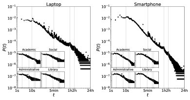
Figure 6: Probability $P\left(t\right)$ of session duration $t$.

VI Traffic analysis

In this section, we compare different traffic characteristics, across device types, time and space. For this purpose, we start with statistical characterization of individual flute and cello flows. Next, we measure how these flows, put together, affect the network patterns across APs and buildings. Finally, user behavior is analyzed by monitoring weekly cycles, data rates, and active durations. By quantifying temporal and spatial variations of traffic across device types, we make a case for new models to capture such variations based on the most relevant attributes. Table IV summarizes the results.

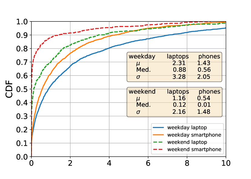
(a) Packet processing rate of APs
(millions per day)

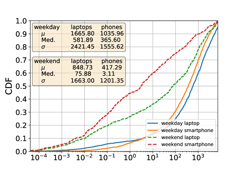
(b) Traffic load of APs
(MB per day, log-scale)

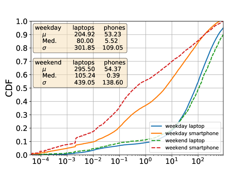
(c) User data consumption
(MB per day, log-scale)

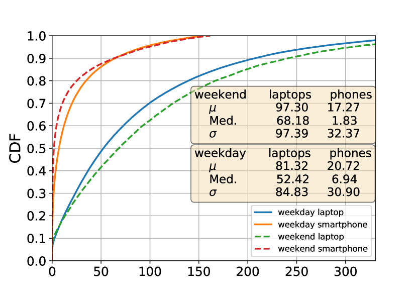
(d) User active time
(minutes per day)

Figure 7: Distribution plots

VI-A Flow-level statistical characterization

We compare the following distributions using maximum likelihood estimation (MLE) and maximizing goodness-of-fit estimation: Gaussian, Exponential, Gamma, Weibull, Logistic, Beta and Lognormal.

VI-A1 Size

Flow size is the sum of bytes for all packets within a single flow. On weekdays, average size of individual flute flows is $>2x$ larger than cello flows ($2070$ vs. $822$ bytes), while median is $>4x$ larger ($678$ vs. $142$ bytes). There are no significant changes on weekends.

The average packet size within a single flow also provides insight into packet-level behavior of services on mobile devices. We notice that the average packet size of flute flows is $\approx$50% larger than that of cellos (212 vs 144 bytes on weekdays, 205 vs 142 on weekends). Comparing weekdays and weekends, median size of flute packets drops on weekends whereas it remains the same for cellos. In fact, comparing cello flows on weekdays and weekends shows no significant difference in terms of average packet size (p-value$>.05$). Despite smaller flows, the average cello generates 2.7 times traffic as an average flute because the average cello is responsible for 3.7 as many flows as a flute. Analyzing distributions of flow size and average packet size in our datasets shows that Lognormal distribution is the best fit, with varying parameters for each device type (More details in Sec. IV of appendices).

VI-A2 Packets

This metric is the count of packets within each flow. The mean and median packet counts per flow are $7.06$ and $5$ in flutes and $3.64$ and $2$ in cellos, during weekdays. The means drop slightly on weekends. Packet counts per flow match the Lognormal distribution well for flows of both device types. The average flute flow is bigger in size and has more packets (with higher variance) but there are fewer flows coming from these devices. This is analyzed further for TCP/UDP flows (Sec. VI-A5).

VI-A3 Runtime

Flow runtime is the period of time the flow was active (equal to a flow’s $finishtime-starttime$). Flute flows have a mean and median of $1868$ms and $128$ms respectively on weekdays, while these numbers are $1639$ms and $64$ms for cellos. Both device types show increase in means during weekends (flutes by $204$ and cellos by $164$), indicating that although there are fewer devices online during weekends, they are more active. The low medians in either group corresponds to many short-lived flows with few packets, showing little variation across device type, time or space.

VI-A4 Inter-arrival times (IAT)

Median of the flow IAT at APs is $6$ms for cello flows and $4$ms in case of flutes, on weekdays (similar on weekends), which suggests that the majority of APs handle flows from either device type at nearly the same rate. However, average IAT is $\approx 143$ms for flute and $\approx 78$ms for cello flows, as there are more cellos with very high rate of flows. Flow IAT in our datasets matches a beta distribution well (See appendix IV) with a very high estimated kurtosis and skewness (estimated at 58 & 6.9 respectively). The high estimated kurtosis illustrates that there are infrequent extreme values, which explains the observed highly elevated standard deviation of IAT. Higher average IAT of flutes, combined with the higher standard deviation compared to cellos (596 vs 284), shows that flutes face more extreme periods of inactivity, which can be caused by higher mobility and packet loss.

VI-A5 Protocols

TCP accounts for 78.5% of cello flows (84.6% of bytes) and 98.2% of flute flows (91.6% of bytes). The higher presence of UDP in cellos is reasonable, considering that UDP applications (e.g., multi-player games, video conferencing and file sharing) are more likely to be used with cellos. Comparing the number of packets in flows, in case of TCP, the average number of packets in cello flows is almost half that of a flute flow (4.6 vs 8.8), and the average packet size of flutes is 22% higher than that of cellos. This supports our earlier observation regarding the bigger flow sizes of flutes. However, for UDP, the two device types are similar in terms of average packet count per flow (2.5 for cellos & 2.87 for flutes) and average packet size (119 for both). This conforms to low latency requirements of many UDP applications.

Given these differences, traffic classification using machine learning [25] could benefit from considering device types to train models. We investigate this in Sec. VII-B.

After establishing the similarities and differences of flows, the next step is to evaluate whether the individual variations in flows lead to different aggregate traffic behaviors from viewpoint of the network.

VI-B Network-centric (spatial) analysis

We examined the load of APs in all buildings on a daily basis to provide insight into differences from the viewpoint of the network. For each AP, we calculate flow metrics for every weekday and weekend.We focus our analysis on the first three weeks of NetFlow traces to avoid significant user behavior change during exams period, as already shown in Fig. 2.

First, we measure the daily packet and flow arrival rates at APs. The median flow rates are $42k$ and $20k$ per weekday for cellos and flutes respectively (7.5k and 0.5k on weekends). The average number of cello packets processed daily by APs is 1.6 times higher than flute packets (Fig. 7(a)). Each AP handles, on average during weekdays, $\approx 27$ cello packets per second and $\approx 17$ flute packets per second, dropping to $\approx 13.5$ and $\approx 6.25$ on weekends. This indicates that, during the weekends, a high percentage of access points are not utilized, with 60% of APs seeing no flute flows and 70% receiving no cello flows. However, at least one AP in $>$80% of buildings sees traffic, supporting observations of less mobility during weekends.

Next, we look at traffic volume. On average weekdays, 90% of APs handle < $5GB$ of cello traffic ($2.5GB$ on weekends), whereas the same percentage handles < $3GB$ of flute traffic ($1GB$ on weekends) (Fig. 7(b)). Flutes are more mobile, visit a higher number of unique APs and have bigger flow sizes but they are still responsible for less overall network load.

Thus, the individual differences of flute and cello flows result in heterogeneous aggregate traffic patterns in time (different days) and space (APs at different buildings). With that established, in order to take steps towards modeling and simulation, we also need to analyze the behavior of users.

VI-C User behavior (temporal) analysis

Here, we measure traffic patterns from a user-centric perspective. We identified gaps in diurnal and weekly cycles (Fig. 2) as well as traffic flow features of individual users including data consumption, packet rates, and network activity duration.

VI-C1 Data consumption

Fig. 7(c) shows daily data consumption, with 90% of cellos consuming < 700MB and 90% of flutes using < 200M on weekdays. Surprisingly, for cellos on campus during weekends, average data consumption is even higher whereas data consumption of flutes drops sharply.

VI-C2 Packet rate

On weekdays, cellos on average generate $\approx$318K packets, while flutes only average $\approx$84K packets per day. On weekends, the few on-campus cellos see greatly increased number of packets, with an average daily packet rate of $\approx 495$K. Weekend flutes also have a modestly increased packet count, with an average of $\approx 96$K flows.

VI-C3 Active duration

Total active time of devices serves well to demonstrate the differences between time spent online by users of different device types. We rely on NetFlow to measure ’active’ time instead of AP association time. This allows us to distinguish user’s idle presence in the network from its activity periods. Cellos have 4x average active time compared to flutes in our traces ($\approx 81$ vs $\approx 21$ min on weekdays, $\approx 97$ vs $\approx 17$ min on weekends). Overall, 90% of cellos are active for $<$3.5h and 90% of flutes are active for $<$1h (Fig. 7(d)). As evident in various metrics, the cellos appearing on weekends are more active than the average cello on weekdays.

Overall, the data consumption of flutes seems to be more bursty in nature, with bigger flows and lower active duration. This could be due to more intermittent usage of flutes and also bundling of network requests to save battery on these devices. In addition, there are fewer devices on campus during weekends, but those remaining devices are more active and consume more data than average.

VII Integrated mobility-traffic analysis

We study the relation between mobility and network traffic features, examine whether their fusion provides a case for the necessity of integrated mobility-traffic models, and introduce steps towards such models (Sec. VII-B).

VII-A Feature engineering

To simplify analysis and interpretation, and reduce dimensionality, we identify the most important features. First, we study the relationships among variables from mobility and traffic dimensions separately. Then, from this subset of combined features, we investigate whether clusters of user devices appear in the dataset. For this, we use correlation feature selection (CFS [26]), to obtain uncorrelated features, but highly correlated to the classification. Finally, we quantify correlations between mobility and traffic metrics (See abbreviations in Fig. 8). Pearson correlation is shown in the figures.

VII-A1 Mobility

The CFS algorithm was run on 8 features (in Sec. V), and kept only 5 (to be used in the cross-dimension analysis). Fig. 8a visualizes the linear dependence between mobility features, comparing flutes and cellos on weekdays and weekends. Close inspection reveals temporal correlation relationships. For example, for cellos on weekends, there is a strong correlation ($0.96$) between preferred building time (PDT) and time of network association (DLT), but weak correlation ($0.1$) on weekdays, suggesting that most of weekend online time is spent at preferred buildings (e.g., libraries).

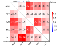
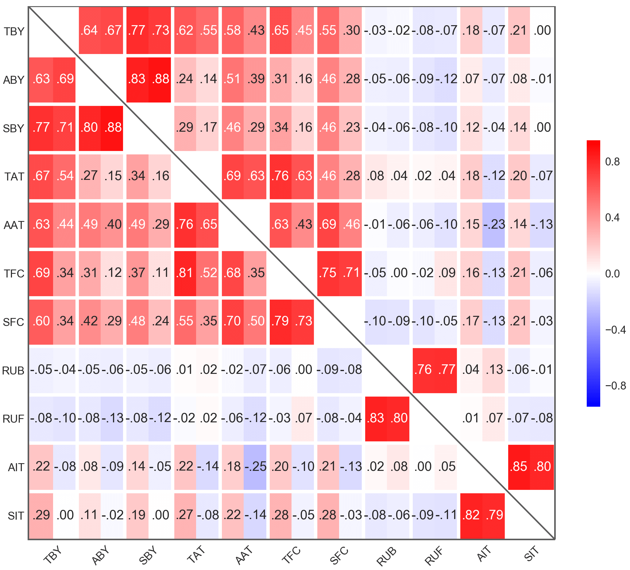
			Abbr. Description TBY Total flow bytes ABY Avg. flow bytes SBY Std. flow bytes TAT Total active time AAT Avg. active time TFC Total flow count SFC Std. flow counts RUB UDP bytes / total bytes RUF UDP flows / total flows AIT Avg. IAT SIT Std. IAT
Abbr. Description APC AP Count (unique) PDT Preferred building $\Delta t$ TJM Total (sum) jumps DIA Diameter of mobility DLT Delta time (time of network association)
(a) Mobility		(b) Traffic

Figure 8: Correlation plots for (a) mobility and (b) traffic features. Each cell’s left half is for flutes and right half is for cellos, the upper right triangle is for weekdays and the lower left for weekends.

TABLE IV: Traffic features used for integrated mobility-traffic analysis (per device, per day; see Fig. 8 for abbreviations). Upper values are for weekdays and lower ones for weekends (in red).

	Flutes (F)			Cellos (C)			Ratio (C/F)
	$\mu$	mdn	$\sigma$	$\mu$	mdn	$\sigma$	$\mu$	mdn
TBY [MB]	96.77	11.47	194.52	373.08	144.68	554.54	3.85	12.61
	80.96	0.86	195.15	448.87	180.23	623.86	5.54	209.56
ABY	5.48	0.74	14.02	15.67	7.34	25.81	2.85	9.91
	4.54	0.15	14.16	18.06	8.34	28.71	3.97	55.6
SBY	10.56	1.57	23.76	30.59	13.77	49.82	2.89	8.77
	8.09	0.13	21.48	33.21	15.42	53.39	4.10	118.61
TAT	1,330	388.6	2,517	5,123	3,003	6,444	3.85	7.73
	1,059	90.89	2,497	5,883	3,861	6,934	5.55	42.48
AAT	63.14	27.97	86.69	188.26	166.93	138.70	2.98	5.96
	50.60	12.98	85.27	206.89	184.17	156.53	4.08	14.18
TFC [K]	7.2	1.7	15.61	33.5	17.1	60.10	4.65	10.05
	5.7	0.3	15.01	38.5	20.6	88.52	6.75	68.66
SFC	515.6	177.3	907.7	1,640	1,181	2,081	3.18	6.66
	361.05	30.18	796.6	1,673	1,215	2,098	4.63	40.27
RUB	0.05	0.00	0.19	0.07	0.00	0.22	1.4	N/A
	0.06	0.00	0.22	0.08	0.00	0.23	1.33	N/A
RUF	0.07	0.00	0.18	0.12	0.02	0.22	1.71	N/A
	0.09	0.00	0.22	0.13	0.02	0.24	1.44	N/A
AIT	3.36	2.24	3.59	3.40	2.45	3.51	1.01	1.09
	2.95	1.74	3.60	3.18	2.27	3.39	1.07	1.3
SIT	5.22	3.44	5.50	5.14	3.18	5.28	0.98	0.92
	4.09	1.98	5.06	4.72	2.79	4.96	1.15	1.41

VII-A2 Traffic

We extract statistical measures for traffic metrics (Sec. VI) per device per day. The CFS algorithm was run on 19 features, reducing them to 11. A summary of these metrics is provided in Table IV. The correlations are depicted in Fig. 8b. The analysis shows us that average number of packets and bytes are positively correlated, but negatively correlated with variance of bytes and uncorrelated with IAT. Average IAT (AIT) seems to be mostly independent from other traffic features, but as AIT increases, its standard deviation (SIT) also greatly increases which could be due to device mobility; bearing further investigation on traffic-mobility interactions. Interestingly, active time is weakly correlated with number of flows and packets, which shows that users who remain online longer are not necessarily consuming traffic at a high rate. Examining weekdays and weekends, correlation trends among traffic features remain similar for either device type.

VII-A3 Cross-dimension

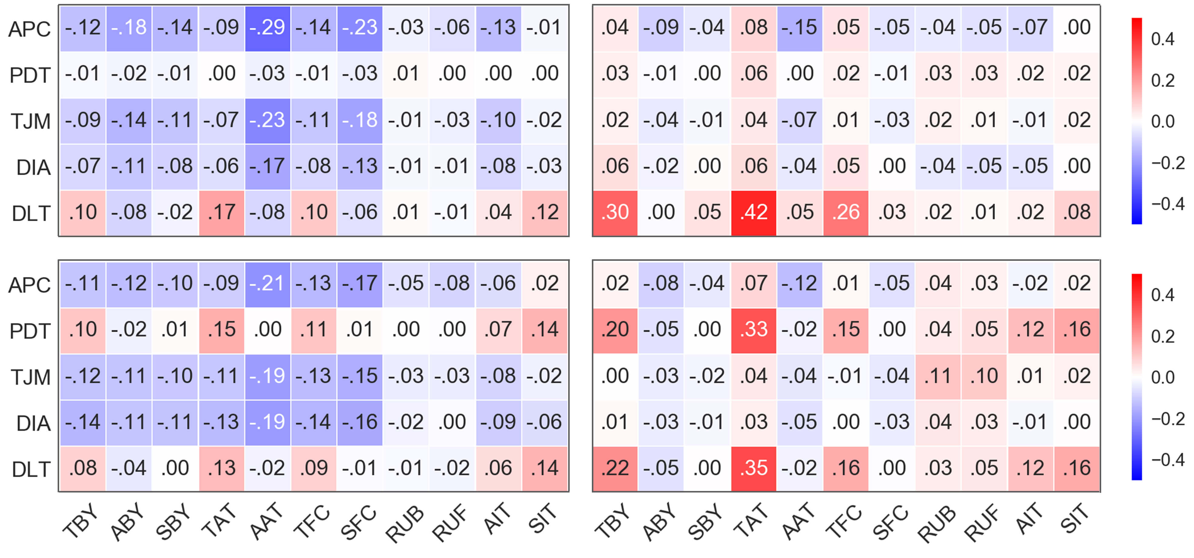
Figure 9: Correlation plots of mobility vs. traffic on weekdays (top) vs. weekends (bottom) for flutes (left) and cellos (right).

Studying correlations across mobility and traffic dimensions, based on subsets of features selected by CFS, is a solid step towards an integrated mobility-traffic model. Results are presented in Fig. 9. We find that as the numbers of unique APs/buildings visited (APC, BLD) increase, the average active time (AAT), and total and std. of flow counts (TFC and SFC) decrease markedly (significant negative correlation). Surprisingly, there is no noticeable change in total traffic consumed with change in APC, suggesting bundling of more packets in flute flows. (Similar correlation between mobility diameter and the above traffic features) Average IAT (AIT) of flutes also rises slightly as mobility metrics decrease; for cellos this correlation is almost nonexistent. This reinforces our “stop-to-use” categorization; cellos are movable but are not active in transit. To sum, flutes score high on mobility metrics, have an overall lower flow count and network traffic but produce bigger flows on average. For cellos, on weekends the more time spent at preferred buildings the higher the total active time (TAT) and flow counts; this effect exists to a lesser degree for flutes. On weekdays, such correlation does not exist.

VII-B Steps towards modeling

Here we present our steps towards an integrated mobility-traffic model, with various applications in simulation and protocol design. We utilize daily mobility and traffic features of users during a week. First, we examine how different mobility and traffic features are for flutes and cellos using machine learning. Second, we investigate whether natural convex clusters of users appear in the dataset. These steps verify that the differences of mobility and traffic characteristics across device types are significant. We also find that combining mobility and traffic makes this distinction even more clear. Finally, mixture models are used to model and synthesize simulated data points of each device type, finding that the accuracy the mixture model increases when trained on combined features.

1. Supervised classification: Having shown significant differences throughout this study, we used support vector machines (SVM) on different subsets of features to examine the feasibility of device type inference as well as the relationship between mobility and traffic characteristics. These sets include mobility and traffic features separately, then combined, and then combined with weekend/weekday labels. Using solely mobility features achieves $\approx$65% accuracy, while traffic features alone, obtains $\approx$79% accuracy. Using all mobility and traffic variables combined, the trained model achieves $\approx$81% accuracy. Then, as the combined feature set is extended to include weekdays and weekends independently, accuracy increases to $\approx$86%. This suggests that users’ behavior (both flutes and cellos) is more distinguishable when looking at combined mobility and traffic features; especially when temporal features such as weekdays are considered separately from weekends. We note that such behavior gaps are not the same for both device types and a model should to take that into account.

2. Unsupervised clustering: To investigate natural convex clusters, we used K-means algorithm. Using mobility features only, the best mean silhouette coefficient is achieved on k=2 and 4. However, cluster sizes are highly skewed and at k=2, $\approx 60\%$ of devices are correctly clustered. Traffic features alone, at k=2, results in $\approx 81.2\%$ accuracy. Combining mobility and traffic, increases the accuracy to $\approx 81.5\%$. While some flutes and cellos are similar in terms of mobility and traffic, the clusters of the combined features clearly illustrate two distinct modes (especially in traffic) and the high homogeneity of the clusters hints at disjoint sets of behaviors in mobility and traffic dimensions, governed by the device type.

3. Mixture model: To take a step towards synthesis of traces based on our datasets, we trained Gaussian mixture models (GMM) on combined mobility and traffic features. From the combined model ($CM$), we acquired simulated samples. We used Kolmogorov-Smirnov (KS) statistic to compare the simulated samples with the real data and found that $CM$ is able to capture the behaviors of each device type. (Average KS statistic of features is $\approx 0.15$ for flutes and $\approx 0.14$ for cellos. More details in appendix V.) Importantly, the combined model produces samples whose traffic features match the original data better, compared with training a GMM on traffic features alone (based on KS statistic), hinting at a key relationship between mobility and traffic. However, comparing mobility features of $CM$ with a GMM trained on mobility features alone shows no improvement.

   Overall, this suggests that there is significant potential for an integrated mobility-traffic model that captures the differences and relationships of features, across device types, time and space. We leave detailed comparison of combined modeling with separate modeling of mobility and traffic for future work.

VIII Conclusion

In this study, we mine large-scale WLAN and NetFlow logs from a campus to answer: (I) How different are mobility and traffic characteristics across device types, time and space? (II) What are the relationships between these characteristics? (III) Should new models be devised to capture these differences? And, if so, how? We build FLAMeS, a framework for systematic processing and analysis of the datasets. Using MAC address survey, OUI matching and web domain analysis, we categorized devices: flutes (“on-the-go”) and cellos (“stop-to-use”). We then study a multitude of mobility and traffic metrics, comparing flutes and cellos across time and space. On average, flutes visit twice as many APs as cellos, while cellos generate $\approx$2x more flows. However, flute flows are 2.5x larger in size, with $\approx$2x the number of packets. The best fit distribution for location preference is Zipfian, for flow/packet sizes is Lognormal, and for flow IAT at APs is beta. Furthermore, flute traffic drops sharply on weekends whereas many cellos remain active. Across mobility and traffic dimensions, we spot a negative correlation for flutes between mobility and flow duration but negligible correlation with traffic size; for cellos, this effect is less pronounced. We find a negative correlation with APs visited and active time, particularly for flutes. However, no correlation exists between APs visited and traffic for cellos. We quantified correlations across both mobility and traffic. Finally, we applied machine learning and trained a mixture model to synthesize data points and verified that the combined mobility-traffic features capture the differences in metrics better than either mobility or traffic separately. Many of our findings are not captured by today’s models, and they provide insightful guidelines for the design of evaluation frameworks and simulations models. Hence, this study answered the questions posed, introduced a strong case for newer models, and provided our first step towards a future integrated mobility-traffic model.

Acknowledgments: We thank Alin Dobra for help in the computing cluster, and the anonymous reviewers for useful feedback. Mostafa Ammar suggested the term ’cello mobility’. Partial funding was provided by NSF 1320694 at Univ. of Florida, August-Wilhelm Sheer fellowship at Technical University-Munich, and Aalto Univ. We also thank Tim Bohne of Osnabrück University for pointing out mistakes in the text.

Appendices

Here we further describe various aspects of our submitted work to Infocom 2018, which were not included in the original document for brevity.

I Merging Datasets

In order to study network traffic across devices and APs, it is necessary to match the NetFlow records with wireless associations (from WLAN dataset). This task requires the MAC-IP mapping. The IP addresses are dynamically assigned using DHCP but DHCP session logs were not directly available and had to be derived. We define the duration of a DHCP lease as the time between two consecutive associations of a device with any AP; i.e. when a device connects to $AP_{1}$, a session starts and once the user device connects to $AP_{2}$, the first session ends and a new one starts. Fig. 10 illustrates the associations of a sample device with different APs at different times. The first session would have the IP given by $AP_{1}$ and a lease time $t_{2}-t_{1}$, and so on. (total of 5 sessions in this example) The last association is discarded as we do not know the duration of that IP assignment. Combining these derived-DHCP records with the Location Information and Device Type Classification we create the DHCP table.

Figure 10: Wireless association for a device at different times.

The derived DHCP and NetFlow datasets were then merged to form what we refer to as the CORE dataset for our study. The unique identifiers between the two are the clients’ IPs in addition to start and end time of flows, hence the need for a DHCP-like set. For a DHCP lease session LS, all flows whose IP address is the same as the lease and whose entire lifetime falls within the lease duration, are associated with LS.

Given these traces, cellular usage cannot be analyzed. However, this does not significantly impact analysis for two reasons: 1) The traces already capture a very large user-base, with tens of thousands of active devices. This raises confidence in our analysis of a real world WLAN. 2) The WiFi campus coverage is ubiquitous, with 1760 APs installed in the vast majority of populated areas. Also, most laptops on campus lack cellular connectivity, and many smartphones use WiFi for their data to avoid cellular data costs.

II Computing System

The size of the datasets is $\approx$30TB in raw text format, mostly consisting of NetFlow data and $\approx$0.5TB for AP logs. There were several challenges in managing and mining the largescale datasets that required a thorough preparation, to run on a fast machine with plenty of resources/memory. We explored several techniques and pipelines for extraction, transformation, loading (ETL) and querying of big data and chose tools from Apache Hadoop ecosystem. We use Hive as our data warehouse (tables stored in Parquet format). Apache Spark is the compute engine for data processing and analysis tasks. Computation runs on two nodes, each with 64 cores and $\approx$0.5TB of memory. Further discussion of the system and comparison to others is out of scope of this document.

III Mobility Analysis

For completeness, we include further analysis of the mobility aspects of our dataset, discussed in Section V of the conference paper.

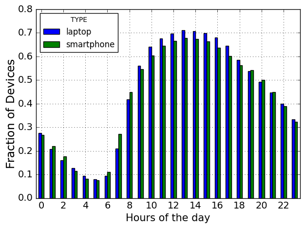
(a)

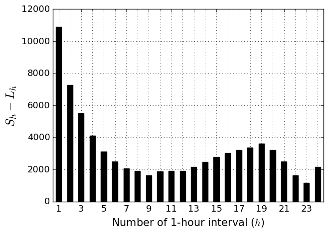
(b)

Figure 11: Hourly associations.

III-A Hourly associations

Measuring device associations every hour, Fig. 11(a) shows the percentage of devices with at least one event as a function of hours of the day. The majority of devices appear online between 9am and 8pm, with the hours between 2am and 6am having less than 20% of devices associating. We find no major differences between flutes’ and cellos’ distributions, as many users potentially own both. As users arrive on campus and their phones announce their first location, they switch on their laptops. This issue bears further research through a future census study.

To measure the stay of devices throughout a day, we look at 1-hour intervals, and measure the number of hours a device accessed an AP . Fig. 11(b) depicts $S_{h}-L_{h}$, where $S_{h}$ and $L_{h}$ are total number of flutes and cellos respectively, with at least one record per hour, as a function of the number of hours online $h$. Flutes are predominant for short visits and very long stays, but the difference drops significantly at 9 hours, then increases. The rise after 9 hours is likely due to students living on campus, with always-on connected phones.

III-B Visitation preferences

(a)

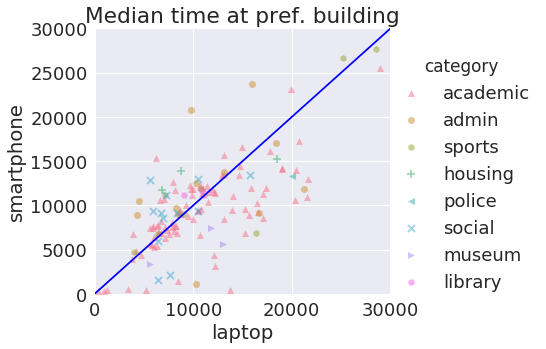
(b)

Figure 12: Time spent at preferred building.

Fig. 12(b) shows a scatter of the median time spent at a user’s preferred building. Each dot represents this value for a given location. This plot shows that academic, police and museum buildings tend to have laptops staying longer, which makes sense intuitively, with students using laptops during lectures and staff working at the other two categories. On the contrary, for social and housing buildings, there is a higher probability of having flutes staying longer, hinting at a tendency to use mobile devices more in such places. Finally, administrative, sports and library buildings tend to have both types of devices staying for similar amounts of time. Analysis of inherited differences in browsing of online services given by this heterogeneity among buildings is left for future work.

Fig. 12(a) depicts the time devices spend at their preferred building in a day.

III-C Return probability

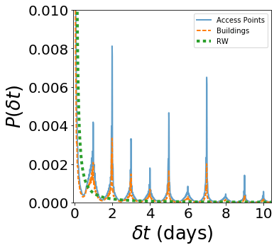
Figure 13: Probability to return to a previously visited location.

We compare empirical values for devices to return to previously visited APs or buildings in Fig. 13. We observe returning spikes at every 24 hours, with the highest peaks at 48 and 168 hours (2 and 7 days). This can be explained by the schedule of classes at the university.

IV Traffic Analysis

In this Section, we further discuss references from Section VI of the conference paper.

IV-A Flow sizes

This metric is the sum of bytes for all packets within a single flow. First, outlier data points are removed using a robust measure of scale, based on inter-quartile range (IQR). Looking at individual flows of each device type shows that size of flows that originated from smartphones are significantly different that laptop flows (p-value< .05).

On weekdays, the average size for smartphone flows is 2070 bytes and 822 bytes for laptop flows; with no significant changes on weekends (CDF in Fig. 14). The difference in medians is more pronounced, on weekdays, for smartphones it is 678 bytes while it is 142 bytes for laptops (similar values on weekends).

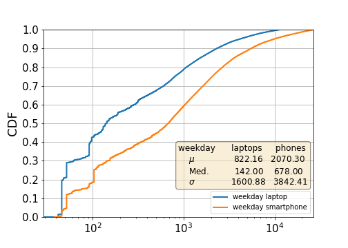
Figure 14: CDF of individual flow sizes (bytes, log-scale $x$ axis), similar pattern on weekends

IV-B Lognormal plots

For flow sizes in our dataset, a Lognormal distribution is the best fit, regardless of device type (Fig. 15). Many models assume flow sizes are static, or follow an exponential distribution but real world data provides no supporting evidence. Such simplifying assumptions fail to accurately account for very large flows obtained from a Lognormal distribution.

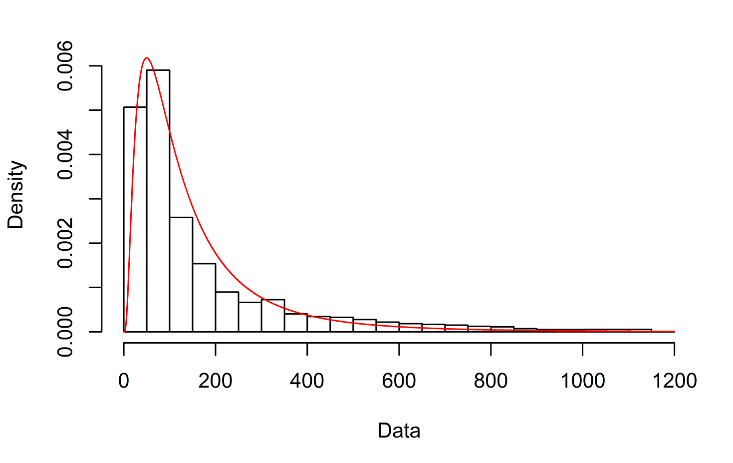
Figure 15: Lognormal distribution.

IV-C beta distribution

Inter-arrival times (IAT). Our results show that the flow IAT, regardless of device type, does not follow an

exponential distribution. Flow IAT matches a beta distribution well (Fig. 16) with a very high estimated kurtosis and skewness (estimated at 58 & 6.9 respectively). The high estimated kurtosis illustrates that there are infrequent extreme values, which explains the observed highly elevated standard deviation of IAT

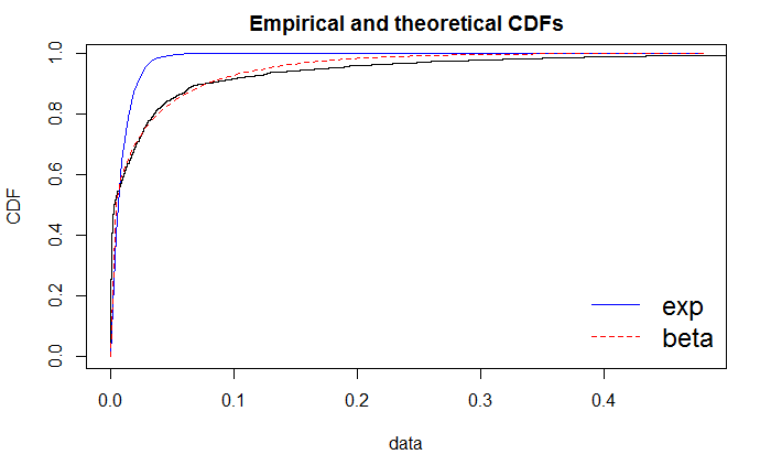
Figure 16: Exponential and Beta distributions.

V First Modeling Steps

More details of the KS test and GMM model are provided here. We found that providing both mobility and traffic features to train a GMM results in lower average KS statistic. Fig 17 shows a sample CDF of TAT. KS statistic details can be found in Table V.

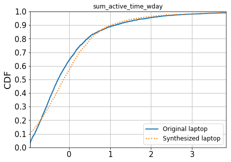
Figure 17: Synthetic vs. Original TAT feature for flutes.

TABLE V: KS-statistic summary

KS statistic	Flutes	Cellos
Average	0.150	0.140
Min	0.052	0.027
Max	0.380	0.350
Std	0.086	0.0787

VI Lessons Learned and Modeling Insights

Our above findings provide further (but surely not yet comprehensive) insights into considerations relevant to the design and parameterization of mobility and network traffic models. While we leave devising and validating a concrete candidate model for future work, we can readily identify the following important elements:

It is crucial to differentiate flutes vs. cellos for both mobility and traffic due to their very different nature. More specifically, flutes exhibit continuous presence whereas cellos are on/off with jumps between locations. Beyond differences in continuity, the traffic patterns (flow sizes, arrival times, etc.) should be specified by device class. Moreover, the traffic generation, spatial locations, and temporal behavior can be linked per device type and per user “community” (e.g. students of different disciplines at various buildings).

Our analyses allow us to quantify the correlated elements of traffic and motion for the (type of) campus we investigated. AP associations allow us to calibrate user mobility and determine their community structures (and “hotspots”), while daily and weekly activity patterns help outline user schedules—which could be parameterized based upon outline information such as class schedules, public holidays, and other predictable events. Traffic flows per device can be created from our corresponding distributions, while AP traffic observations allow parameterizing the above “hotspots” with respect to user activity.

Together, these could form a basis for generating parameters for established mobility models^,, possibly extend them as needed, and augment them with adequate correlated traffic models. The next step is examining the minimum number of parameters required (parsimonious model) to approximate user behavior within given error bounds with respect to the observed ground truth. This should be complemented by studying datasets from other network settings to further validate the observed behaviors beyond our campus environment, taking into account the specifics of the campus and identifying further influencing factors.

Besides different campus environments, a few further elements deserve further study: 1) Our study so far gives only limited insight into the actual services users are accessing, so analyzing web domains users are accessing, for interest and application analysis as well as investigating the relationship of user interests with spatio-temporal characteristics of mobility and traffic would be important next steps. 2) Flutes and cellos are likely two points in a dimension that is continuously changing as a) differentiation in device classes appear (e.g., smartphones vs tablets—do we have “guitars” as well?); b) blur again (e.g., due to new form factors for smartphones and tablets); and c) new devices such as fitness trackers, smart watches and “glasses” further enrich the portfolio.

References

- [1] J. Treurniet, “A Taxonomy and Survey of Microscopic Mobility Models from the Mobile Networking Domain,” ACM CSUR, 2014.
- [2] A. Hess, K. A. Hummel, W. N. Gansterer, and G. Haring, “Data-driven Human Mobility Modeling: A Survey and Engineering Guidance for Mobile Networking,” ACM CSUR, 2016.
- [3] D. Kotz and K. Essien, “Analysis of a Campus-Wide Wireless Network,” Springer Wireless Networks, vol. 11, no. 2, January 2005.
- [4] T. Henderson, D. Kotz, and I. Abyzov, “The changing usage of a mature campus-wide wireless network,” Elsevier Computer Networks, 2008.
- [5] G. Maier, F. Schneider, and A. Feldmann, “A First Look at Mobile Hand-held Device Traffic,” in Proc. of IEEE PAM, 2010.
- [6] Y. Zhand and A. Arvidsson, “Understanding the Characteristics of Cellular Data Traffic,” in ACM SIGCOMM CellNet workshop, 2012.
- [7] S. Moghaddam and A. Helmy, “SPIRIT: A simulation paradigm for realistic design of mature mobile societies,” in IWCMC ’11, 2011.
- [8] M. C. Gonzalez, C. A. Hidalgo, and A.-L. Barabasi, “Understanding individual human mobility patterns,” Nature, vol. 453, no. 7196, 2008.
- [9] C. Song, T. Koren, P. Wang, and A.-L. Barabási, “Modelling the scaling properties of human mobility,” Nature Physics, vol. 6, no. 10, 2010.
- [10] D. Zhang, J. Huang, Y. Li, F. Zhang, C. Xu, and T. He, “Exploring human mobility with multi-source data at extremely large metropolitan scales,” MobiCom ’14.
- [11] G. Maier, F. Schneider, and A. Feldmann, “A first look at mobile hand-held device traffic,” in PAM ’10. Springer, 2010.
- [12] U. Kumar, J. Kim, and A. Helmy, “Changing patterns of mobile network (WLAN) usage: Smart-phones vs. laptops,” IWCMC ’13, 2013.
- [13] X. Chen, R. Jin, K. Suh, B. Wang, and W. Wei, “Network performance of smart mobile handhelds in a university campus wifi network.” IMC’12.
- [14] A. Gember, A. Anand, and A. Akella, “A comparative study of handheld and non-handheld traffic in campus wi-fi networks,” in PAM ’11.
- [15] M. Afanasyev, T. Chen, G. M. Voelker, and A. C. Snoeren, “Analysis of a mixed-use urban wifi network: when metropolitan becomes neapolitan,” in ACM SIGCOMM ’08.
- [16] I. Papapanagiotou, E. M. Nahum, and V. Pappas, “Smartphones vs. laptops: comparing web browsing behavior and the implications for caching,” SIGMETRICS’12.
- [17] H. Falaki, D. Lymberopoulos, R. Mahajan, S. Kandula, and D. Estrin, “A first look at traffic on smartphones,” IMC ’10, 2010.
- [18] A. K. Das, P. H. Pathak, C.-N. Chuah, and P. Mohapatra, “Characterization of wireless multidevice users,” ACM TOIT, 2016.
- [19] P. Cao, G. Li, A. Champion, D. Xuan, S. Romig, and W. Zhao, “On human mobility predictability via wlan logs,” in INFOCOM ’17.
- [20] A. Nikravesh, Y. Guo, F. Qian, Z. M. Mao, and S. Sen, “An in-depth understanding of multipath TCP on mobile devices,” in MobiCom ’16.
- [21] X. G. Meng, S. H. Y. Wong, Y. Yuan, and S. Lu, “Characterizing flows in large wireless data networks,” MobiCom ’04, 2004.
- [22] F. Xu, Y. Li, H. Wang, P. Zhang, and D. Jin, “Understanding mobile traffic patterns of large scale cellular towers in urban environment,” IEEE/ACM Transactions on Networking, April 2017.
- [23] A. W. Moore and D. Zuev, “Internet traffic classification using bayesian analysis techniques,” SIGMETRICS ’05, vol. 33, no. 1, 2005.
- [24] V. Paxson and S. Floyd, “Wide area traffic: the failure of Poisson modeling,” IEEE/ACM ToN, vol. 3, no. 3, jun 1995.
- [25] T. Nguyen and G. Armitage, “A survey of techniques for internet traffic classification using machine learning,” IEEE CST’08.
- [26] M. A. Hall, “Correlation-based feature selection for machine learning,” Ph.D. dissertation, The University of Waikato, 1999.
- [27] W.-J. Hsu, T. Spyropoulos, K. Psounis, and A. Helmy, “Modeling time-variant user mobility in wireless mobile networks.”
- [28] P. Widhalm, Y. Yang, M. Ulm, S. Athavale, and M. C. González, “Discovering urban activity patterns in cell phone data,” Transportation’15.
- [29] C. Boldrini and A. Passarella, “Hcmm: Modelling spatial and temporal properties of human mobility driven by users’ social relationships,” Computer Communications, vol. 33, no. 9, 2010.