Disks Around Merging Binary Black Holes: From GW150914 to Supermassive Black Holes

Abstract

We perform magnetohydrodynamic simulations in full general relativity of disk accretion onto nonspinning black hole binaries with mass ratio $q=29/36$. We survey different disk models which differ in their scale height, total size and magnetic field to quantify the robustness of previous simulations on the initial disk model. Scaling our simulations to LIGO GW150914 we find that such systems could explain possible gravitational wave and electromagnetic counterparts such as the Fermi GBM hard X-ray signal reported 0.4s after GW150915 ended. Scaling our simulations to supermassive binary black holes, we find that observable flow properties such as accretion rate periodicities, the emergence of jets throughout inspiral, merger and post-merger, disk temperatures, thermal frequencies, and the time-delay between merger and the boost in jet outflows that we reported in earlier studies display only modest dependence on the initial disk model we consider here.

I Introduction

Accreting black holes are central in explaining a range of high-energy astrophysical phenomena that we observe in our Universe, such as X-ray binaries, active galactic nuclei (AGN), and quasars. Recently, substantial theoretical and observational effort has gone into understanding accretion onto binary black holes and the emergent electromagnetic (EM) signatures these systems may generate, because they are anticipated to exist at the centers of distant AGNs and quasars (see, e.g., Gold et al. (2014a) for a summary of relevant work prior to 2014, and Zilhão et al. (2015); Farris et al. (2015); Nguyen and Bogdanović (2016); Kulkarni and Loeb (2016); Rafikov (2016); Bowen et al. (2017); Ryan and MacFadyen (2017); Haiman (2017); D’Orazio and Di Stefano (2017); Kharb et al. (2017); Bowen et al. (2017) and references therein for some more recent work). The bulk of the research so far has focused on supermassive black holes binaries and about 150 candidate accreting supermassive black hole binaries have been identified in quasar surveys Graham et al. (2015); Charisi et al. (2016); Graham et al. (2015). Depending on the physical properties of the above systems, such as the mass ratio and orbital period, some of these candidates may be in the gravitational-wave driven regime D’Orazio et al. (2015). However, in addition to accreting supermassive binary black holes, there may exist black hole binaries of a few tens of solar masses that could be accreting matter from a circumbinary disk. This scenario has attracted a lot of attention recently because of the direct detection of gravitational waves (GWs).

In particular, on September 14, 2015, the LIGO and Virgo collaborations made the first direct detection of a GW signal – event GW150914 Abbott et al. (2016). GW150914 was entirely consistent with an inspiraling and merging binary black hole (BHBH) in vacuum as predicted by the theory of general relativity (GR). This detection provided the best evidence yet for the existence of black holes. Meanwhile, the detection of a transient EM signal (event GW150914-GBM) at photon energies $>50$ keV that lasted 1 s and appeared 0.4 s after the GW signal was reported in Connaughton et al. (2016), who used data from the Gamma-ray Burst Monitor (GBM) aboard the Fermi satellite. The Fermi GBM satellite was covering 75% of the probability map associated with the LIGO localization event in the sky, thus this signal could be a chance coincidence. We note that while the detection of GW150914-GBM has been controversial (see e.g. Xiong (2016); Greiner et al. (2016)), a recent reanalysis of the data reported in Connaughton et al. (2016) finds no reasons to question it con (2018). On the other hand, an MeV-scale EM signal lasting for 32 ms and occurring 0.46 s before the third GW detection made by the LIGO detectors (event GW170104) – also consistent with a BHBH Abbott et al. (2017) – was reported in Verrecchia et al. (2017), who used data from the AGILE mission. While these candidate counterpart EM signals were not confirmed by other satellites operating at the same time, they still excited the interest of the community and several ideas about how to generate accretion disks onto “heavy” black holes, such as those that LIGO detected, have been proposed.

Circumbinary disks were proposed because inspiraling and merging BHBHs in vacuum do not generate EM signals, but they may do so in the presence of ambient gas, such as binaries residing in AGNs Bartos et al. (2017); Stone et al. (2017) or those with gas remaining from their stellar progenitors Perna et al. (2016); Loeb (2016); Murase et al. (2016); Li et al. (2016). There are multiple papers that suggest possible connections between LIGO GW150914 and GW150914-GBM, see, e.g., Loeb (2016); Janiuk et al. (2017a, b). Sources that could generate both the GWs and the hard X-rays reported include binary black hole-neutron stars, binary black hole-massive stars, and rapidly rotating massive stars. In Fedrow et al. (2017); Dai et al. (2016); Ackermann et al. (2016) constraints on the resulting BHBH and ambient gaseous environment are discussed. However, some of these constraints may not account for all the physical processes involved, thus accretion onto BHBHs under a wide number of scenarios may still be relevant not only for supermassive black holes found in AGNs, but also for LIGO’s heavy black holes. Future “multimessenger” observations of such systems will better inform us regarding the existence of accreting heavy BHBHs.

In previous work Farris et al. (2012); Gold et al. (2014a, b) we initiated magnetohydrodynamic (MHD) studies of nonspinning binary black holes accreting from a circumbinary disk in full GR. We modeled both the binary-disk predecoupling and post-decoupling phases. We investigated the effects of magnetic fields and the binary mass ratio, and discovered that these systems launch magnetically driven jets (even though the black holes were nonspinning) whose Poynting luminosity is of order 0.1% of the accretion power. Therefore, these systems could serve both as radio, X-ray and gamma-ray engines for supermassive BHBHs in AGNs and as gamma-ray-burst-like engines for LIGO-observed BHBH masses, if in the latter case the hyperaccreting phase associated with the merger lasts for $O(1\rm s)$. We also discovered that $\sim 2-5(M/10^{8}M_{\odot})(1+z)$ d [or $\sim 0.1-0.3(M/65M_{\odot})(1+z)$ s] following merger, there is a significant boost both in the Poynting luminosity and the efficiency for converting accretion power to EM luminosity. The time delay in units of M between merger and the jet luminosity boost, as well as the magnitude of the boost, depends on the binary mass ratio. In particular, more equal-mass binaries exhibit a longer time delay and stronger boost. The origin of this boost is currently unclear. It could be due to the fact that, prior to merger, the black holes in our simulations were nonspinning, while after merger a single, spinning black hole formed. It could also be due to an increase of magnetic flux accreted onto the BHs prior to and after merger, as the binary tidal torques modify the accretion flow – the higher the mass ratio the weaker the tidal torques and the more magnetized matter is present in the vicinity of the binary prior to merger. It has never been explored whether this time delay depends on the initial disk model. For example, one could anticipate some dependence on the disk thickness because the binary tidal torques depend on the disk thickness, as well (see e.g. Kocsis et al. (2012a, b); Armitage and Natarajan (2002); Liu and Shapiro (2010); Kocsis et al. (2012, 2012); Shapiro (2013)).

In this paper we consider a black hole binary with mass ratio $q=29/36$ – motivated by the inferred value of the mass ratio of GW150914 – and consider different initial disk models to explore their impact on the emergence of jets, the outgoing Poynting luminosity, the presence of periodicities in the accretion rate, and the time delay between merger and the boost in the jet luminosity that we discovered before. As in our previous studies we ignore the disk self-gravity and detailed microphysics, which then allows us to scale the binary black hole mass and disk densities to arbitrary values. Thus, our results can be applied to both supermassive black hole binaries and LIGO/Virgo black hole binaries.

Scaling our simulations to the GW150914 mass scale, we find that magnetized accretion onto binary black holes could explain both the GWs detected from this system and the EM counterpart GW150915-GBM reported by the Fermi GBM team 0.4s after LIGO’s GW150915 detection. We also find that flow properties such as the emergence of jets, accretion rate periodicities, temperatures, thermal frequencies, and the time-delay between merger and the boost in jet outflows that we reported in our earlier studies display only modest dependence on the disk model.

The rest of the paper is structured as follows: In Sec. II we provide a qualitative overview of the evolution of a BHBH – accretion disk system to motivate some of the parameters we choose in our simulations. In Sec. III we summarize the methods we adopt for generating initial data and for the dynamical evolution. A general description of our simulation results are reported in Sec. IV. In Sec. V we discuss the astrophysical implications of our findings, both in the context of possible EM counterparts to LIGO/Virgo GW sources and in the context of luminous AGNs. We summarize our conclusions in Sec. VI. Geometrized units, where $G=1=c$, are adopted throughout unless stated otherwise.

II Qualitative Overview

The evolution of a circumbinary disk is roughly composed of three phases: (i) The early inspiral predecoupling phase, during which the disk viscous timescale ($t_{\rm vis}$) is shorter than the GW timescale ($t_{\rm GW}$), and the quasistationary disk tracks the BHBH as it slowly inspirals; (ii) the postdecoupling phase, during which $t_{\rm vis}>t_{\rm GW}$ and the binary decouples from the disk and runs away, leaving the disk behind with a subsequent decrease in the accretion rate; (iii) The post-merger or re-brightening/afterglow phase during which the disk begins to refill the partial hollow left “behind” the BHBH and accretion ramps up onto the spinning remnant BH.

The disk structure at decoupling determines the subsequent evolution and the EM emission. A rough estimate of the decoupling radius for our simulations is obtained by equating the viscous timescale $t_{\rm vis}$ to the GW inspiral timescale $t_{\rm GW}$. The former is approximately given by

$$t_{\rm vis}\sim\frac{2}{3}\frac{R_{in}^{2}}{\nu},$$

where, $\nu$ is the effective kinematic viscosity induced by MHD turbulence, and $R_{in}$ is the radius of the disk inner edge. We can fit the viscosity to an $\alpha$-disk law for an analytic estimate (see Teukolsky and Shapiro (1983)):

$$\nu(R)=\frac{2}{3}\alpha\left(H/R\right)^{2}\left(MR\right)^{1/2},$$

where $H$ is the thickness of the disk. The GW inspiral timescale is given roughly by

$$t_{GW}\approx\frac{5}{64}\frac{a^{4}}{M^{2}\mu},$$

where $a$ is the binary separation, $M$ is the total BHBH mass, and $\mu$ is the reduced mass. Denoting the inner radius of the disk as $R_{in}=\beta a$, we find the decoupling radius $a_{d}$ to be

$$\frac{a_{d}}{M}\approx 13\left(\frac{\beta}{1.4}\right)^{3/5}\left(\frac{M}{4\mu}\right)^{-2/5}\left(\frac{\alpha}{0.13}\right)^{-2/5}\left(\frac{H/R}{0.2}\right)^{-4/5},$$

where the normalizations are based on typical values the parameters obtain in our canonical simulation described below. This estimate suggests that when choosing initial conditions the binary orbital separation should be larger than $13M$. In our simulations we choose an initial separation of $\sim 14M$ and find that decoupling occurs at orbital separations $\sim 10M$, consistent with the above estimate. This allows the BHBH to undergo $\sim 10$ nearly-circular orbits before reaching the decoupling radius $a_{d}$, which in turn, allows the inner disk to relax before decoupling, yielding a quasistationary accretion flow.

Although the above picture regarding the evolution of the matter in the circumbinary disk allows us to estimate the decoupling radius, we point out that recent numerical simulations have challenged it (see e.g. Gold et al. (2014a, b); Farris et al. (2015); Duffell et al. (2014); Edgar (2007)). In particular, it has been found that dense spiral accretion streams are attached onto the BHs during the entire inspiral. Nevertheless, in fully general relativistic simulations of thick accretion disks Farris et al. (2015); Gold et al. (2014b), the accelerated inspiral during the late stages causes the accretion rate to plummet by factors of several. This phase can be taken to signal the ”decoupling” of the binary from the disk and matches the prediction of the last equation.

III Methods

III.1 Metric Initial Data

We prepare the spacetime metric initial data using the TwoPunctures code Ansorg et al. (2004) and choose the puncture momenta such that the BHBH is initially on a quasi-circular orbit at coordinate orbital separation of $\sim 14M$. We choose the puncture bare masses such that the ratio of irreducible masses is $q=29/36$, and set the spins to zero ($a_{1}/M_{1}=0=a_{2}/M_{2}$), which are both consistent with the mass ratio and effective spin $\chi=M_{1}(a_{1}/M_{1})+M_{2}(a_{2}/M_{2})\approx 0$ reported for GW150914. The initial orbital period of the binary is $\sim 368M$, and the total number of orbits until BHBH merger is about 16, (see Tab. 1 for a summary of the BHBH properties).

III.2 Matter and Magnetic-field Initial Data

We set up a magnetized accretion disk as in Gold et al. (2014a). The initial disk configurations we consider would be equilibrium solutions around single nonspinning black holes which have the same mass as the ADM mass of the BHBH, if the disk was not magnetized. In particular, we use the same family of hydrodynamic equilibrium disk models around single black holes discussed in Farris et al. (2011); Villiers et al. (2003), which we construct by adopting a $\Gamma$-law equation of state (EOS), $P=(\Gamma-1)\,\epsilon\,\rho_{0}$. The $\Gamma$-law EOS is also adopted for the dynamical evolution and allows for shock heating. Here $\epsilon$ is the specific internal energy and $\rho_{0}$ the rest-mass density. In all our models we set $\Gamma=4/3$, which is appropriate when thermal radiation pressure dominates and allows for comparisons with our earlier simulations reported in Gold et al. (2014a). More detailed microphysics must be incorporated to replace this simple EOS with a more realistic model, but the adopted $\Gamma$-law EOS suffices for our initial survey in which we wish to understand the basic MHD flow and gross EM luminosity features.

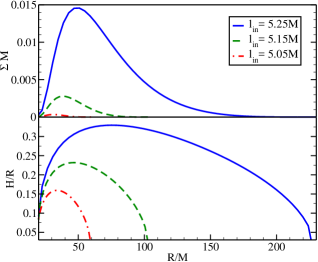
Figure 1: Plots of surface density profile $\Sigma(R)$ and disk scale height $H/R$ vs. cylindrical coordinate radius $R$ for the three disk models. These initial disk models belong to a one-parameter family of models in which the parameter that varies is the specific angular momentum parameter ($l_{\rm in}$) at the disk inner edge, whose initial radius we fix at $20M$. For cases A, B, and C we have $l_{\rm in}=5.25M$ (solid lines), $l_{\rm in}=5.15M$ (dashed lines), and $l_{\rm in}=5.05M$ (dot-dashed lines), respectively (see Tab. 2).

Table 1: Two puncture initial data parameters for the BHBH spacetime. Columns show the mass ratio ($q$), defined as the ratio of the BH irreducible masses ($M_{\rm irr}^{i}$, $i=1,2$), the binary coordinate separation ($a/M$), the binary angular velocity $\Omega M$, and total ADM angular momentum $J/M^{2}$, where $M$ is the total ADM mass. Both BHs are nonspinning.

BHBH Initial Data Parameters
$q=M_{\text{irr}}^{2}/M_{\text{irr}}^{1}$	$a/M$	$\Omega M$	$J/M^{2}$
29/36	13.8	$1.71\times 10^{-2}$	1.07

We consider three cases for the disk model by varying the geometric thickness of the disk. Figure 1 shows the difference between the different disk models via a plot of the initial surface density $\Sigma(R)=\int_{z\geq 0}\rho_{0}u^{t}\sqrt{-g}\,dz$, where $R$ is the cylindrical coordinate radius, and the scale height $H(R)=\Sigma(R)/\rho_{0}(z=0)$. In Tab. 2 we list basic properties of these initial disk models.

By neglecting the disk self-gravity and adopting a $\Gamma$-law EOS, we have the freedom to scale the binary ADM mass and disk densities to any value. But the scaling remains physically valid only when the disk mass $M_{\rm disk}$ is much smaller than the BHBH ADM mass $M$. This scale freedom makes our calculations relevant both for AGN environments and for environments that can explain the observed Fermi GBM luminosity of $\sim 10^{49}$ erg/s reported in Connaughton et al. (2016) (see Appendix A for a discussion of how this scaling works for several physical quantities).

Table 2: Here $l_{\rm in}=-u_{\phi}/u_{t}$ is the specific angular momentum parameter at the inner radius of the disk, $(H/R)_{\text{max}}$ is the maximum disk scale height, and $R_{\rm out}/M$ is the outer radius of the disk. In all cases, the inner radius of the disk is $R_{\rm in}/M=20$.

Initial Disk Parameters
Case	$l_{\rm in}/M$	$(H/R)_{\rm max}$	$R_{\rm out}/M$
A	5.25	0.33	250
B	5.15	0.22	100
C	5.05	0.14	60

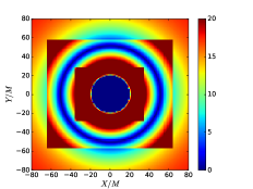
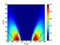
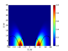
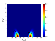
Figure 2: Top row: Contours of the $\lambda_{\text{MRI}}$-quality factor $Q=\lambda_{\text{MRI}}/dx$ in the equatorial plane at $t=0$ for all cases. Bottom row: Rest-mass density contours (color coded) on a meridional slice, and $\lambda_{\text{MRI}}/2$ (black solid line) at $t/M=0$ for all cases. The left column plots correspond to case A, the middle column to case B and the right column to case C. These plots demonstrate that with our grid choices we resolve the fastest growing MRI mode by $\gtrsim 10$ points in the bulk of the disks (the blue ring stems from the extremely small values of $\lambda_{\text{MRI}}$ where the vertical component of the B-field changes sign). The plots also demonstrate that $\lambda_{\text{MRI}}/2$ mostly fits within the disks.

As in Farris et al. (2012), we seed the initial disk with an initially dynamically unimportant, purely poloidal magnetic field that is entirely confined in the disk interior. The initial magnetic field is generated by the following vector potential

$$A_{i} =\left(-\frac{y}{\varpi^{2}}{\delta^{x}}_{i}+\frac{x}{\varpi^{2}}{\delta^{y}}_{i}\right)A_{\varphi}$$ (1)

$$A_{\varphi} =A_{b}\varpi^{2}{\rm max}(P-P_{c},0)$$ (2)

where $\varpi^{2}=x^{2}+y^{2}$, and $A_{b}$, and $p_{c}$ are free parameters. $A_{b}$ is determined by the maximum value of the magnetic-to-gas-pressure ratio which we set to $P_{\rm mag}/P_{\rm gas}\approx 0.022,0.028,0.042$ for cases A, B, C, respectively. We also choose the cutoff pressure $P_{c}$ to be 1% of the maximum pressure. The magnetic field renders the disk unstable to the magnetorotational instability (MRI) that ultimately leads to the development of MHD turbulence. The associated effective turbulent viscosity allows angular momentum to be transported and accretion to proceed. We impose three conditions that enable MRI to operate in our disk models: (i) We choose disk configurations whose rotation profile satisfies $\partial_{R}\Omega<0$, where $\Omega=u^{\phi}/u^{t}$ is the fluid angular velocity Duez et al. (2006). (ii) We resolve the wavelength of the fastest growing MRI mode $\lambda_{\text{MRI}}$ by $\gtrsim$ 10 gridpoints Shibata et al. (2006). Using the initial disk data, we plot the quality factor $Q\equiv\lambda_{\text{MRI}}/dx$, where $dx$ is the local grid spacing, which jumps by a factor of 2 at adaptive mesh refinement (AMR) boundaries. The top panels of Fig. 2 show plots of $Q$ in the equatorial $x-y$ plane for all three cases, demonstrating that $\lambda_{\text{MRI}}/dx>10$. Note that the square patterns are a result of the AMR grids (see below). (iii) The initial B-field is sufficiently weak – $\lambda_{\text{MRI}}\lesssim 2H$, where $H$ is the disk scale height, i.e., the wavelength of the fastest growing mode fits within the disk. The bottom panels in Fig. 2 show meridional xz-slices of the rest-mass density overlayed by a line plot showing $\lambda_{\text{MRI}}/2$ as a function of $x$ for the three cases. For the most part, $\lambda_{\text{MRI}}/2$ fits inside the disk.

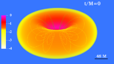
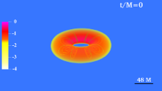
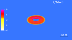
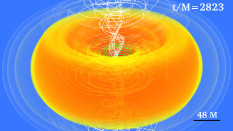
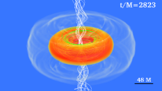
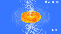
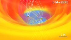
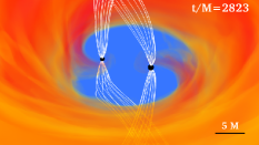
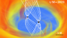
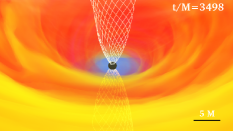
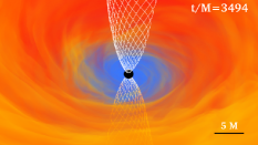
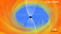
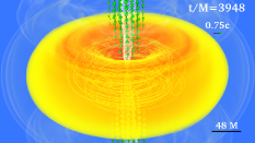
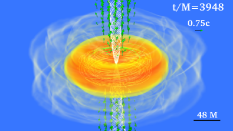
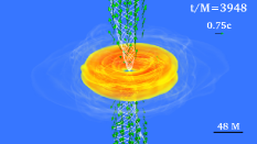
Figure 3: Volume rendering of rest-mass density, normalized to its initial maximum value $\rho_{0,\text{max}}$ (see color coding), magnetic field lines (solid white curves), and velocity vectors (green arrows) at select times during the inspiral, merger and post-merger. Case A corresponds to the left column, case B to the middle column, and case C to the right column.

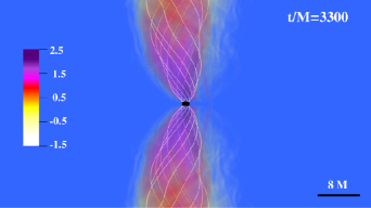
Figure 4: Volume rendering of magnetic-to-rest-mass energy density $\log\left(b^{2}/2\rho_{0}\right)$ for case B. The white lines indicate the magnetic field lines corresponding to the B field measured by a normal observer.

III.3 Dynamical evolution methods

We use the Illinois GRMHD AMR code which is embedded in the Cactus/Carpet infrastructure Cactus ; Carpet and has been developed by the Illinois relativity group Duez et al. (2005); Etienne et al. (2010, 2012a). This code is the basis of its publicly available counterpart embedded in the Einstein Toolkit Etienne et al. (2015). Our code has been extensively tested (including with resolution studies) and used in the past to study numerous systems involving compact objects with and without magnetic fields Etienne et al. (2012b, 2008); Liu et al. (2008); Paschalidis et al. (2011a, b) including black hole binaries in magnetized accretion disks Gold et al. (2014a, b).

For the metric evolution, the code solves the equations of the Baumgarte-Shapiro-Shibata-Nakamura (BSSN) formulation of GR Shibata and Nakamura (1995); Baumgarte and Shapiro (1998) coupled to the moving-puncture gauge conditions Baker et al. (2006); Campanelli et al. (2006) with the equation for the shift vector cast in first-order form (see e.g. Hinder et al. (2014)). The shift vector parameter $\eta$ is set to $\eta=1.375/M$.

For the matter and magnetic field, the code solves the equations of ideal GRMHD in flux-conservative form (see Eqs. 27-29 in Etienne et al. (2010)) employing a high-resolution-shock-capturing scheme. To enforce the zero-divergence constraint of the magnetic field, we solve the magnetic induction equation using a vector potential formulation (see Eq. 9 in Etienne et al. (2012a)). As our EM gauge choice, we use the generalized Lorenz gauge condition developed in Farris et al. (2012). This EM gauge choice avoids the development of spurious magnetic fields that arise across AMR levels (see Etienne et al. (2012) for more details). We set the generalized Lorenz gauge damping parameter to $\xi=7/M$.

To compare with our previous calculations Gold et al. (2014a, b) and to reduce the computational overhead associated with the evolutions, equatorial symmetry is imposed in all cases. Equatorial symmetry does not allow plasma to cross the equatorial plane Etienne et al. (2012b); Yuan et al. (2012); Roberts et al. (2017) and hence limits the development of some modes. We will explore the impact of reflection symmetry on such circumbinary accretion flows in a future investigation. The computational mesh consists of three sets of nested AMR grids, one centered on each BH and one on the binary center of mass (with $9$ levels of refinement in each set). The outer boundary is at $384$M in all cases. The coarsest grid spacing is $\Delta x_{\rm max}=6.0$M. The grid spacing of all other levels is $\Delta x_{\rm max}/2^{n-1},\ n=1,2,\ldots$, where $n$ is the level number such that $n=1$ corresponds to the coarsest level. The half length of each AMR level box is $384{\rm M}/2^{n-1}$ for $n=1,\ldots 5$, and $528{\rm M}/2^{n}$, for $n=6,\ldots,9$.

IV Results

The basic evolution of the BHBH-disk system has previously been described in Farris et al. (2012); Gold et al. (2014a, b), where it was found that when keeping the binary at fixed orbital separation of $10M$ for a disk with initial inner radius $R_{\rm in}=20M$, the accretion rate begins to settle at $t\simeq 2000M$, which signals that the inner disk edge has relaxed. This result motivates in part our choice of initial BHBH orbital separation of $13.8$M, because within a time of 2000M the binary undergoes about 10 orbits and then reaches the orbital separation of $\sim 10M$, at which point the inspiral in Gold et al. (2014b) began, once the disk was allowed to relax. The fact that the initial orbital separation in our current simulations is larger than in our earlier studies implies that the accretion rate is expected to settle even earlier for the same disk model, because the black holes are closer to the disk and hence it is easier for them to tidally strip matter from the inner disk edge. Our simulations confirm this expectation, where for the same initial disk model as in Farris et al. (2012); Gold et al. (2014a) the accretion rate begins to settle at $t\sim 1500M$.

IV.0.1 Evolution of the matter and magnetic fields

Figure 3 shows 3D volume snapshots of the density at selected epochs during the evolution. Soon after the evolution begins we observe the formation of high-density, spiral accretion streams that attach onto the BHs during the entire inspiral and through merger (see the middle row in Fig. 3). In all cases we also observe the emergence of a mildly relativistic, collimated outflow from each black hole. These outflows merge at large heights to form a single helical magnetic-field, incipient jet flow (second row of Fig. 3). As the binary inspirals the incipient twin jets merge more tightly and the inner disk edge flows inward, both helping to collimate the outflow further. After merger a single incipient jet onto the remnant black hole forms (4th and 5th rows in Fig. 3).

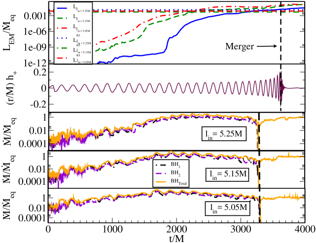
Figure 5: The Poynting luminosity $L_{\rm EM}$ and accretion rate $\dot{M}$ vs. time for all cases and the strain of the “plus” polarization of the gravitational waveform $h_{+}$. The GWs are computed as described in Etienne et al. (2012). The dotted-dashed lines on the top panel indicate the expected Blandford-Znajek luminosity from a single BH with the same mass, spin and quasistationary polar magnetic field-strength as found for each case. The normalization $\dot{M}_{\rm eq}$ in each panel is the time-averaged accretion rate onto the post-merger remnant black hole over the last 500M of the evolution. The displacements in the dashed vertical merger line in the luminosity and GW plots with respect to the merger lines in the accretion plots accounts for the light travel time between the BH and the radiation extraction radii.

IV.0.2 Accretion rates

We compute the accretion rate through the black hole apparent horizons via Eq. (A11) of Farris et al. (2010). Figure 5 shows the accretion rate of all cases as a function of time, along with the outgoing Poynting luminosity. Also shown is the gravitational waveform. The accretion rate reaches a quasisteady state at $t/M\sim 1500$ for all cases, and the average accretion rate remains approximately constant for the next $1000$M of evolution, consistent with the system being in the “predecoupling” phase, as anticipated. During this phase a Fourier transform indicates that the accretion rate exhibits a periodicity at periods equal to $202$M, $210$M and $202$M for cases A, B and C, respectively. These periods equal $\simeq 0.8P$, where $P$ is the average orbital period, $P\simeq 250$M, which we determine from the GWs during this predecoupling epoch. Notice that the dominant period in the accretion rate being smaller than the binary orbital period is consistent with our findings in Gold et al. (2014a). The $\sim 0.8P$ accretion rate periodicity has been associated with a “lump” feature in earlier work Noble et al. (2012); Roedig et al. (2012). However, we have reported accretion periodicities at $0.7-0.8P$ in earlier work of ours Gold et al. (2014a) even in cases where a lump was absent. Thus, there may be more than one mechanism that can explain this periodicity. We plan to address this point with targetted simulations in a future work. The fact that for different disk models the accretion rate modulation occurs at approximately the same period indicates that this signature is not sensitive to the adopted disk models. At $t\sim 2500M$, the inspiral of the BHs begins to speed up, and the accretion rate begins to drop, indicating the onset of the “postdecoupling” phase. At the time of merger the total accretion rate drops, but soon after merger, the low-density hollow begins to fill up, increasing the accretion rate after merger.

Following merger, for the thinnest disk case during the time evolved the accretion rate achieves a steady-state value at $\sim 3\%$ of the maximum accretion rate during the evolution. For the middle disk the post-merger accretion rate is $\sim 14\%$ of the maximum accretion rate achieved during evolution; for the thicker disk this value is $\sim 30\%$. A careful resolution study is necessary to assess the significance of this result, which we defer to a future investigation.

IV.0.3 Outflows and jets

In all three cases we find that at $t\sim 2500$M after the start of the simulations, collimated and magnetically dominated outflows emerge in the disk funnel independently of the disk model. The timescale over which these incipient jets emerge is consistent with those we reported in Farris et al. (2012); Gold et al. (2014a, b). The incipient jets persist through inspiral, merger and post-merger, as seen in Fig. 3. During merger we find that the magnetization in the funnel grows and after the merger the magnetization reaches $b^{2}/2\rho_{0}\gtrsim 100$, indicating that the jets are magnetically powered. Here $b=B/4\pi$ with $B$ the magnetic field measured by a comoving observer, and $\rho_{0}$ is the rest-mass density. The region above and below the BH remnant is nearly force-free – a prerequisite for the Blandford-Znajek (BZ) mechanism Blandford and Znajek (1977). A representative plot of $b^{2}/2\rho_{0}$ and the magnetic field lines in the funnel is shown in Fig. 4. Associated with these outflows is a large scale outgoing Poynting flux.

We calculate the outgoing Poynting luminosity on the surface of coordinate spheres $S$ as $L_{(EM)}=\oint_{S}T_{0,\,(EM)}^{\,\,\,r}dS$, where $T_{\mu,\,(EM)}^{\,\,\,\nu}$ is the EM stress-energy tensor. $L_{(EM)}$ as a function of time is shown in Fig. 5 for all cases. Following binary merger, the luminosity ramps up to a nearly constant value in all cases for the duration of the simulation. After merger, we find that the “efficiency” $\epsilon_{\rm EM}\equiv L_{\rm EM}/\dot{M}_{\rm eq}$ ($\dot{M}_{\rm eq}$ is the time-averaged accretion rate onto the post-merger remnant BH over the last 500M of the evolution) increases as the disk thickness decreases. However, we note that since our goal here is to test the robustness of global BHBH-disk features across different disk models, we did not prepare initial disks with the same initial amount of poloidal magnetic flux, which has been found to be one of the major determining factors for the efficiency of the outgoing Poynting luminosity in MHD BH accretion disks (see e.g. Beckwith et al. (2008); McKinney et al. (2012)).

In Gold et al. (2014b) we discovered that following merger there is a boost in the jet power by a factor 3-4 with time delay in units of M between merger and the boost that depends on the mass ratio. In particular, we found that the more unequal mass BHBHs, the shorter the time delay in units of M, which ranges between $\sim 350$M (for $q=4$) and $\sim 1000$M (for $q=1$). Here, we discover that the boost in the Poynting luminosity and the existence of a time delay between merger and the boost is robust among the different disk models we consider in this work. In our study the time delay is $\sim 600$M for cases A and B, and $\sim 300$M for case C, suggesting that for fixed mass ratio and thick disks, the time delay between merger and boost in EM luminosity exhibits only modest dependence on the disk thickness.

After the boost and the outgoing Poynting luminosity achieve a quasiequilibrium, the Poynting luminosity is comparable to the EM power expected from the BZ effect:

$$L_{\rm BZ}\sim 10^{48}\left[\frac{(a/M_{\rm BH})}{0.68}\right]^{2}\left(\frac{M_{\rm BH}}{62M_{\odot}}\right)^{2}\left(\frac{B_{p}}{4\times 10^{12}\rm G}\right)^{2}\rm ergs^{-1}$$ (3)

(see Eq. 4.50 in Thorne et al. (1986)). We plot $L_{\rm BZ}$ normalized to the post-merger accretion rate averaged over the last 500M in the top panel of Fig. 5, taking the remnant BH dimensionless spin and mass values from our simulations, while adopting for the magnetic field above the BH poles $B_{p}$, its time-averaged value over the last 500M of evolution.

As mentioned earlier, above the remnant BH poles the funnel is nearly force-free ($B^{2}/8\pi\rho_{0}\gg 1)$). The BZ solution has been found to approximately describe the force-free regions in the funnel of magnetized, geometrically thick disks accreting onto single, spinning BHs McKinney and Gammie (2004); De Villiers et al. (2005), thus, we can attribute this luminosity and accompanying incipient jet from the remnant spinning BH-disk system to the BZ effect. During the inspiral a “kinetic” or “orbital” BZ effect can account for the outgoing EM energy Palenzuela et al. (2010).

V Astrophysical implications

In this section we discuss the implications of our results to astrophysical systems of interest, ranging from black hole binaries relevant to LIGO to supermassive black hole binaries that likely reside at the centers of AGNs and quasars.

V.1 LIGO GW150914

Table 3: Table for the maximum rest-mass density $\rho_{0}^{max}$, disk rest-mass to BHBH mass ratio $M_{\text{disk}}/M_{\text{BH}}$, post-merger, time-averaged accretion rate $\dot{M}_{\rm eq}$ over the last 500M of the evolution, maximum equivalent isotropic luminosity $L_{\rm iso}$ after merger, the magnetic-field strength measured by an observer comoving with the plasma averaged over a cube of side equal to the remnant coordinate BH apparent horizon radius $r_{\rm AH}$ and located immediately above the remnant BH at the end of the simulation, and the time $\tau_{\text{delay}}$ between merger and peak luminosity.

Simulation Results (for GW150914)
Case	$\rho_{0}^{\text{max}}$ (g cm${}^{-3})$	$M_{\text{disk}}/M_{\text{BH}}$	$\dot{M}_{\rm eq}$ ($M_{\odot}$ s-1)	$L_{\rm iso}$ (erg s-1)	$B_{p}$ (G)	$\tau_{\text{delay}}$ (s)
A	$2.4\times 10^{5}$	$1.1\times 10^{-3}$	$3.3\times 10^{-4}$	$1.8\times 10^{49}$	$8.6\times 10^{12}$	0.2
B	$1.9\times 10^{5}$	$1.9\times 10^{-4}$	$0.8\times 10^{-4}$	$1.8\times 10^{49}$	$3.6\times 10^{12}$	0.2
C	$1.8\times 10^{6}$	$4.2\times 10^{-4}$	$0.7\times 10^{-4}$	$1.8\times 10^{49}$	$4.1\times 10^{12}$	0.1

In this subsection we investigate whether circumbinary BHBH accretion disks could explain simultaneous GW and EM signals of the type GW150914 and GW150914-GBM. For the BHBH-disk model to explain the GW150914-GBM event, the following minimum set of requirements must be met: i) the accretion rate has to be high enough to explain to observed luminosity, ii) the densities have to be sufficiently low for “dynamical friction” not to alter the BHBH inspiral and hence the waveforms, and iii) the model has to explain why Fermi GBM did not see any EM signal before merger.

Point i) is trivial to account for within the BHBH-disk models described here, utilizing our allowed scale freedom. We scale the BHBH ADM mass in our simulations to correspond to the event GW150914, i.e., $65M_{\odot}$. Therefore, the individual BH masses become $M_{\rm BH,1}=36M_{\odot}$, and $M_{\rm BH,2}=29M_{\odot}$. In addition, we scale the maximum rest-mass density in the disk so that the EM luminosity in our models matches the inferred equivalent isotropic luminosity of $\sim 1.8\times 10^{49}$ erg s^-1 for the GW150914-GBM event Connaughton et al. (2016), assuming a beaming angle of 20 degrees (the approximate jet opening angle in our simulations) and a $10\%$ conversion efficiency to observable photons (see Appendix A for how such scaling is performed). To be precise we assume that the equivalent isotropic luminosity $L_{\rm iso}$ corresponding to the EM flux ($f$) detected by Fermi GBM is related to the total Poynting luminosity $L_{\rm EM}$ according to

$$\frac{L_{\rm iso}}{4\pi D_{L}^{2}(z)}=\frac{\epsilon L_{\rm EM}/2}{2\pi\eta_{c}D_{L}^{2}(z)}$$ (4)

where $\epsilon$ is the fraction of the Poynting luminosity that becomes hard X-ray photons, $\eta_{c}=1-\cos(\theta)$ (with $\theta$ the jet half-opening angle) is a “collimation” factor, which equals 0.06 for a $\theta=$20 degrees, and $D_{L}(z)$ is the luminosity distance. The factor of $1/2$ in the numerator in the right-hand-side of Eq. (4) arises because Fermi GBM would see only the jet directed towards it, whereas the luminosity output we compute is from both jets. Equation (4) yields

$$L_{\rm EM}=\frac{\eta_{c}L_{\rm iso}}{\epsilon}$$ (5)

We then set $L_{\rm EM}$ such that $L_{\rm iso}=1.8\times 10^{49}\rm erg\ s^{-1}$, $\eta_{c}=0.06$, and $\epsilon=0.1$, a fiducial value.

Table 3 shows physical quantities for each of the cases using this scaling. In the predecoupling phase, the accretion rate reaches $\sim 10^{-3}M_{\odot}s^{-1}$ for all disk models, and after merger the rates settle approximately to the same value, $\sim 10^{-4}M_{\odot}s^{-1}$. The maximum rest-mass densities in the disks are $\sim 10^{5}$g cm^-3 for cases A and B, and $\sim 10^{6}$g cm^-3 for case C. Note also, that the maximum attainable value of the Lorentz factor $\Gamma_{L}$ for steady-state, axisymmetric jets approximately equals the quantity $B^{2}/(8\pi\rho$) Vlahakis and Königl (2003), which can reach values of $\gtrsim 100$ within the funnel.

In Fedrow et al. (2017) it is argued that for the scenario where an accreting BHBH system is formed through stellar core fragmentation, at gas densities $\rho\gtrsim 10^{6}-10^{7}$ g cm^-3, dynamical friction between the BHs and the gas will change the coalescence dynamics and the GW signal in a measurable way. However, in the relativistic simulations presented in Fedrow et al. (2017) the initial BHBH was immersed in a nonrotating, constant density cloud, employing prototype densities that could arise in an evolved progenitor star. In other words, the binary did not form self-consistently following fragmentation inside a massive progenitor star. Nevertheless, Tab. 3 shows that one can explain the GW150914-GBM luminosity with rest-mass densities $\lesssim 10^{6}$ g cm^-3, which according to Fedrow et al. (2017) would not affect significantly the GW signal. Our study also suggests that models with thicker tori, such as those encountered following stellar collapse Shibata et al. (2006); Sun et al. (2017), may require lower densities and stand a better chance at explaining both the GW and the EM signals from GW150914-GBM.

Another consistency check we must perform is that GW150914-GBM appeared about 0.4 s following the BHBH merger observed by the LIGO detectors. However, we find that magnetized BHBH-disk systems have jet output before merger whose power increases as the binary approaches merger and after merger. Note that the increasing EM power output as the orbital separation decreases that we discovered in Farris et al. (2012); Gold et al. (2014b), and is also present here, is consistent with the findings reported recently in Kelly et al. (2017), who studied BHBH mergers in magnetized clouds. The question then is: if the BHBH-disk model is able to explain the multimessenger signatures of the GW150914-GBM event, why did Fermi GBM not observe an EM signal during the inspiral phase? The fact that GW150914-GBM was a marginal (3$\sigma$) detection allows for the possibility that the signal before merger was not sufficiently strong to trigger Fermi GBM. In Paschalidis (2017) it was pointed out that the time delay of about $1000$M$\sim 0.3($M$/65M_{\odot})$ s between merger and the boost in the jet luminosity found in earlier BHBH-disk simulations Farris et al. (2012); Gold et al. (2014b) could explain this delay in the GW150914-GBM signal in the sense that it could be weak enough prior to merger and grow strong enough to be detectable only after merger.

To assess this possibility for the models we consider here, we compute the energy flux Fermi GBM would detect as a function of time as follows

$$f=\frac{\epsilon L_{\rm EM}/2}{2\pi\eta_{c}D_{L}^{2}(z)}.$$ (6)

In all estimates, we choose a fiducial value of $\epsilon=0.1$ and $\eta_{c}=0.06$, and set the maximum $L_{\rm EM}$ through Eq. (5). Figure 6 shows the EM flux vs time curve for each case at redshift $z=0.09$. The plot also shows an estimate for the Fermi GBM 1s sensitivity (horizontal line). Note that for all cases Fermi GBM would detect the burst occurring post-merger but not during the inspiral, which is consistent with the observation Connaughton et al. (2016). Notice also that the time delay to reach the peak luminosity after merger is of order 0.2 seconds, which is also consistent with GW150914-GBM. The time delay is due to the fact that the binary carves out a low density hollow which is roughly the same for most disk models. Therefore, this time delay, during which the hollow is filled by accreting gas, is likely universal.

The last aspect one has to account for is the duration of the burst. In principle, the EM burst duration is likely to be connected to the engine lifetime which in our scenario is the accretion disk. The disk accretion time in our models is $O(100\rm s)$, and hence much longer than the GW150914-GBM burst duration of 1s. This is because we did not carefully design our disk models to match all aspects of the scenario considered. The accretion timescale depends on the net magnetic vertical flux inside the disk which determines the effective alpha viscosity and the accretion rate (for a fixed luminosity and fixed efficiency of converting accretion power to EM power). The timescale also depends on the density distribution in the disk, the specific angular momentum profile etc. This large parameter space must be explore in order to be able to find the right disk model, i.e., the one which yields the desired accretion time. Recent simulations of collapsing massive stars in full general relativity Sun et al. (2017), find accretion timescales of order 1s when scaled to $M=65M_{\odot}$. Moreover, the simulations of Reisswig et al. (2013) that form black hole binaries from fragmenting, collapsing stars in full general relativity, find accretion disks with accretion timescales $\sim 0.3$ s, when scaled to $65M_{\odot}$. Thus, it is likely that an appropriate disk model can be found, and a more promissing approach for building the disk model is to start with matter initial conditions that approximate the tori found in such self-consistent calculations Sun et al. (2017); Reisswig et al. (2013). The topic requires further investigation and we plan to tackle it in a future work.

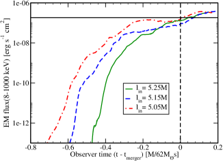
Figure 6: GBM flux vs. time for each case assuming the source lies at redshift $z=0.09$. The dashed vertical line is the time at which the binary merges as measured by the observer. The horizontal line shows the sensitivity of Fermi GBM.

Extrapolating from our recent compact binary simulations modeling short gamma-ray burst (sGRB) engines Paschalidis et al. (2015); Ruiz et al. (2016) and supermassive star  Sun et al. (2017), a unified analytic model was proposed in Shapiro (2017) to crudely explain some of the most significant global parameters characterizing engines formed from compact binary mergers and stellar collapse. We present a comparison of our findings with the model of Shapiro (2017) in Appendix B adopted for GW150914-GBM.

V.2 Supermassive binary black holes

In the following, we scale the BHBH ADM mass to equal $M=10^{8}M_{\odot}$. GWs from such supermassive BHBHs may be detected ultimately by the spaced based LISA detector Amaro-Seoane (2013); Amaro-Seoane et al. (2017), targeting GW frequencies $10^{-5}-1\rm Hz$, as well as Pulsar Timing Arrays et. al. (2010); Tanaka et al. (2012); Sesana (2013), targeting GW frequencies $10^{-9}-10^{-6}\rm Hz$. The GW strain for a $q=29/36$ mass ratio binary at orbital separation $d=10M$ is $h\sim 10^{-16}(M/10^{8}M_{\odot})(D_{L}/6.7\rm Gpc)^{-1}$, where $D_{L}$ is the luminosity distance and the normalization chosen corresponds to redshift $z\simeq 1$ in a standard $\Lambda$CDM cosmology. The corresponding GW frequency is $f_{\rm GW}\sim 6.5\times 10^{-5}\left(M/10^{8}M_{\odot}\right)^{-1}[(1+z)]^{-1}$Hz, with merger frequency $f_{\rm GW,merger}\sim 6.5\times 10^{-4}\left(M/10^{8}M_{\odot}\right)^{-1}[(1+z)]^{-1}$Hz. The merger time from $d=10M$ is $\sim 4(M/10^{8}M_{\odot})(1+z)$d. This GW strain is above the LISA sensitivity at these frequencies Amaro-Seoane (2013), hence these systems may be detectable by LISA. Moreover, with proper modeling, EM precursor signals can trigger targeted GW searches in the LISA band with a substantial lead time, should such systems merge frequently enough. Conversely, LISA can also localize a source on the sky weeks before merger, and then wide-field telescopes will have a comfortable lead time to monitor the area Kocsis et al. (2012a, b); Lang and Hughes (2009). However, we note that binaries with mass $\sim 10^{6}-10^{7}M_{\odot}$ are more promising LISA sources. On the other hand binaries with masses $10^{9}-10^{10}M_{\odot}$ are promising sources for Pulsar Timing Arrays et. al. (2010); Tanaka et al. (2012); Sesana (2013).

We now also scale the maximum rest-mass density in the disks to be $\rho_{0}=5.6\times 10^{-11}$ g cm^-3, which gave a Poynting luminosity near the Eddington limit in Gold et al. (2014a). Table 4 shows that the accretion rates found here are in the range $10^{-7}-10^{-9}M_{\odot}$ s^-1 but the Poynting luminosity is near the Eddington luminosity. Only case C we consider deviates by an order of magnitude from the Eddington luminosity.

Table 4: Table of values for the maximum rest-mass density $\rho_{0}^{\rm max}$, disk-BH mass ratio $M_{\text{disk}}/M_{\text{BH}}$, accretion rate $\dot{M}$, luminosity $L$ in units of the Eddington luminosity $1.26\times 10^{46}(M/10^{8}M_{\odot})$ (erg s^-1), the magnetic-field strength measured by an observer comoving with the plasma averaged over a cube of side equal to the remnant coordinate BH apparent horizon radius $r_{\rm AH}$ and located immediately above the remnant BH at the end of the simulation, and the time $\tau_{\text{delay}}$ between merger and peak luminosity. Note that the quantities listed in the table scale with the BH mass and density as listed in the footnotes.

Simulation Results (Supermassive BHBH Scaling)
Case	$\rho_{0}^{\text{max}}$ g cm-3	$M_{\text{disk}}/M_{\text{BH}}$	$\dot{M}$ ($M_{\odot}$ s-1)	$L_{\rm EM}/L_{\rm edd}$	$B_{p}$ (Gauss)	$\tau_{\rm delay}/(1+z)$
A	$5.6\times 10^{-11}$	$6.7\times 10^{-7}$	$2.0\times 10^{-7}$	$0.9$	$1.3\times 10^{5}$	3.6 d
B	$5.6\times 10^{-11}$	$1.4\times 10^{-7}$	$6.2\times 10^{-8}$	$1.0$	$6.1\times 10^{4}$	3.6 d
C	$5.6\times 10^{-11}$	$3.4\times 10^{-8}$	$6.0\times 10^{-9}$	$0.1$	$2.3\times 10^{4}$	1.8 d

For all models, the characteristic effective temperature in the bulk of the disk is approximately insensitive to the disk model or inspiral epoch and is similar to what we reported in Gold et al. (2014a) and Gold et al. (2014b):

$$T_{\rm eff}\sim 10^{5}\left(\frac{L_{\rm EM}}{L_{\rm Edd}}\right)^{1/4}\left(\frac{M}{10^{8}M_{\odot}}\right)^{-1/4}{\rm K},$$ (7)

where we assumed $\rho_{0}\epsilon=aT^{4}$, to estimate the local temperature, and we set $\rho_{0}$ as in Gold et al. (2014a). Note that these temperatures are only crude estimates, because we do not account for microphysics here. In our calculations, the temperature is also position dependent and is close to $6\times 10^{5}(M/10^{8}M_{\odot})^{-1/4}$K near the inner disk edge and goes to $2-3\times 10^{5}(M/10^{8}M_{\odot})^{-1/4}$K in the bulk of the disk. So, the order of magnitude is $10^{5}$K. In some recent Newtonian calculations with more detailed radiation microphysics (e.g. Farris et al. (2015); Tang et al. (2018)) the temperatures obtained are somewhat higher. But those calculations are all in 2D and based on alpha-disk viscosity laws and not on 3D GRMHD as performed here, with magnetic fields providing the effective turbulent viscosity, and this may account for the difference. The corresponding characteristic thermal radiation frequencies ($\nu_{\rm bb}\sim k_{B}T_{\rm eff}/h$) are given by

$$\nu_{\rm bb}\sim 10^{15}\left(\frac{M}{10^{8}M_{\odot}}\right)^{-1/4}\left(\frac{L_{\rm b}}{L_{\rm Edd}}\right)^{1/4}(1+z)^{-1}\rm Hz.$$ (8)

Current and future EM detectors such as PanStarrs et. al. (2002), the LSST LSST Science Collaboration et al. (2009) and WFIRST Green (2012) could detect such thermal EM signals.

VI Conclusions

We performed MHD simulations of binary black holes with mass ratio $q=29/36$ that accrete magnetized matter from a circumbinary accretion disk. We consider three initial disk models that differ in their scale heights, physical extent and in their magnetic field content in order to test whether previous properties of MHD accretion flows onto binary black holes are sensitive to the initial disk model. We find that the presence of periodicities in the accretion rate, the emergence of jets, the time delay between merger and the boost in the jet luminosity that we previously discovered Farris et al. (2012); Gold et al. (2014a, b) are all robust features and largely insensitive to the choice of initial disk model.

As in our previous studies we ignored the disk self-gravity and adopted a simplified $\Gamma$-law EOS ($\Gamma=4/3$), which allows us to scale the binary black hole mass and disk densities to arbitrary values. Thus, our results have implications both for LIGO black-hole binaries and for supermassive black hole binaries at centers of luminous AGNs and quasars.

Scaling our simulations to LIGO GW150914 we find that magnetized disk accretion onto binary black holes could explain both the GWs detected from this system, and the EM counterpart GW150915-GBM reported by the Fermi GBM team 0.4s after LIGO’s GW150915. When scaling to supermassive black hole binaries, we find that at late times flow properties, temperatures, thermal frequencies, are all robust displaying only modest dependence on the disk model. Nevertheless, the range of disk thickness and ratio of magnetic-to-gas pressure in our survey is limited by what we can achieve with current computational resources and methods. As computational resources grow and numerical techniques advance we will be able to probe wider ranges of these parameters.

Using the remnant BH-disk parameters found for the simulations, we also tested the predictions of the unified model presented in Shapiro (2017) for gamma-ray bursts formed from compact binary mergers and massive star collapse. We found that the disk accretion rate, Poynting luminosity, EM radiation efficiency and the disk lifetimes are in rough agreement between the model and the simulations.

Appendix A Scaling with Rest-Mass Density

Our model may be scaled to arbitrary rest-mass density $\rho_{0}$ because we neglect the self-gravity of the disk and we adopt a $\Gamma$-law EOS. The density everywhere is determined by specifying its maximum value, $\rho_{0}^{\rm max}$, which can be set by requiring that once the remnant black hole and disk achieve quasistationary equilibrium, $L_{\rm EM}=L_{\rm EM\text{ (observed)}}$. Quantities such as the accretion rate and EM luminosity are provided in code units, and then $\bar{\rho}_{{\rm max}}$ is rescaled to establish the luminosity condition and $M_{\rm BH}$ to equal the desired binary ADM mass. Here and below we consider barred quantities to be given in code units. Knowing how all other quantities scale with $\rho_{0}^{\rm max}$ and $M_{\rm BH}$ then allows us to rescale their values appropriately. Below we show how their scaling with $\rho_{0}^{{\rm max}}$ and $M_{\rm BH}$ is established.

The accretion rate $\dot{M}$ onto the merger remnant black hole scales as

$$\dot{M}\sim\rho_{0}M_{BH}^{2}\Rightarrow\frac{\dot{M}_{\rm BH}}{\bar{\dot{M}}_{\rm BH}}=\frac{\rho_{0}}{\bar{\rho}_{0}}\left(\frac{M_{BH}}{\bar{M}_{BH}}\right)^{2}.$$ (9)

To show that $P_{\rm gas}$ must scale with $\rho_{0}$, we begin with the fact that we adopt a $\Gamma$-law EOS,

$$P_{\rm gas} =(\Gamma-1)\rho_{0}\epsilon$$

$$=(\Gamma-1)\rho_{0}\left(h-1-\frac{P}{\rho_{0}}\right)$$

where $\epsilon$ is the specific internal energy, and $h=1+\epsilon+P/\rho_{0}$ is the specific enthalpy. Now using $P_{\rm gas}=K\rho_{0}^{\Gamma}$, we solve for $P_{\rm gas}/\rho_{0}$ to get

$$\frac{P_{\rm gas}}{\rho_{0}}=\frac{\Gamma-1}{\Gamma}(h-1)$$ (10)

As shown in  Farris et al. (2011), $h=h(r,\theta)$ is fixed, dimensionless, and completely determined by the initial parameters $R_{\rm in}$, $l_{\rm in}$, and $q$ (see Eq. A12 in Farris et al. (2011)). The right-hand-side of Eq. 10 is then a constant, and hence

$$\frac{P_{\rm gas}}{\bar{P}_{\rm gas}}=\frac{\rho_{0}}{\bar{\rho}_{0}}$$ (11)

Now in our simulations, we set the maximum value of the ratio $P_{\rm mag}/P_{\rm gas}$ at $t=0$, where $P_{\rm mag}=B^{2}/8\pi$. Hence, to preserve this ratio upon rescaling, we have

$$\frac{B}{\bar{B}}=\left(\frac{\rho_{0}}{\bar{\rho}_{0}}\right)^{1/2}.$$ (12)

Finally, since $L_{\rm EM}\sim B^{2}M_{\rm BH}^{2}$, we have

$$\frac{L_{\rm EM}}{\bar{L}_{\rm EM}}=\frac{\rho_{0}}{\bar{\rho}_{0}}\left(\frac{M_{BH}}{\bar{M}_{BH}}\right)^{2}.$$ (13)

Thus when we may set $L_{\rm EM}=L_{EM\text{ (observed)}}$, and use Eq. 13 to rescale the maximum rest-mass density after determining $\rho_{0}/\bar{\rho}_{0}$. Then we can use Eqs. 9, 11, and 12 to compute the remaining quantities.

Appendix B Comparison with simple estimates

Table 5: Order of Magnitude Comparison of Simulation Results with Model in Shapiro (2017).

Case	$L_{\rm EM}/\dot{M}_{\rm eq}$		$t_{\text{disk}}/M_{\rm BH}$		$\rho M_{\rm BH}^{2}$		$B_{p}^{2}M_{\rm BH}^{2}$
	Shapiro (2017)	Simulations	Shapiro (2017)	Simulations	Shapiro (2017)	Simulations	Shapiro (2017)	Simulations
A	$0.01$	0.01	$10^{6}$	$10^{6}$	$10^{-14}$	$10^{-12}$	$10^{-12}$	$10^{-13}$
B	$0.01$	0.1	$10^{5}$	$10^{5}$	$10^{-13}$	$10^{-12}$	$10^{-12}$	$10^{-13}$
C	$0.01$	0.1	$10^{6}$	$10^{6}$	$10^{-13}$	$10^{-12}$	$10^{-12}$	$10^{-14}$

Recently a unified analytic model was proposed in Shapiro (2017) to explain several key global parameters characterizing an accretion disk–black hole system that can launch a jet consistent with the BZ mechanism Blandford and Znajek (1977). The model accounted for disk-black hole systems formed either through compact binary mergers or massive star collapse. Here we apply the model to the case of GW150914. The inferred characteristic disk parameters for a viable BH-disk system for GW150914, which has a low isotropic luminosity ($\sim 10^{49}$ erg s^-1), are given in Eq. 19 of Shapiro (2017) as

$$\begin{split}&\frac{M_{\rm disk}}{M}\sim 1\times 10^{-5},\ \ \frac{R_{\rm disk}}{M}\sim 20,\\ &{\dot{M}_{\rm eq}}\sim 0.9\times 10^{-3}~{}M_{\odot}~{}{\rm s^{-1}}.\end{split}$$ (14)

Here $R_{\rm disk}$ is roughly identified with the outer radius of the disk. The inferred values are determined by matching the model to the observed luminosity and lifetime of GW150914-GBM, ignoring beaming and off-axis viewing.

The value for the accretion rate is within an order of magnitude of the value our simulations predict here in order to match the luminosity of GW150914-GBM (see Tab. 3).

In geometrized units the model of Shapiro (2017) generally predicts

$$\dot{M}_{\text{eq}}\sim 4\left(\frac{M_{\text{disk}}}{M}\right)\left(\frac{M}{R_{\text{disk}}}\right)^{3},$$ (15)

and

$$L_{BZ}\sim\frac{1}{10}\left(\frac{M_{\text{disk}}}{M}\right)\left(\frac{M}{R_{\text{disk}}}\right)^{3}\left(\frac{a}{M}\right)^{2},$$ (16)

and hence

$$\frac{L_{BZ}}{\dot{M}_{\rm eq}}\sim\frac{1}{40}\left(\frac{a}{M}\right)^{2},$$ (17)

(Eqns. 11-13 of Shapiro (2017)).

The model also predicts a characteristic disk density and the magnetic field strength near the BH poles:

$$\rho M^{2}\sim\frac{1}{\pi}\left(\frac{M_{\rm disk}}{M}\right)\left(\frac{M}{R_{\rm disk}}\right)^{3},$$ (18)

$$B_{p}^{2}M^{2}\sim 8\left(\frac{M_{\rm disk}}{M}\right)\left(\frac{M}{R_{\rm disk}}\right)^{3}$$ (19)

(Eqs. 9 and 10 of Shapiro (2017)).

The model also predicts for the disk lifetime

$$t_{\text{disk}}/M\sim\frac{(M_{\rm disk}/M)}{\dot{M}_{\rm eq}}\sim\frac{1}{4}\left(\frac{R_{\text{disk}}}{M}\right)^{3}$$ (20)

In table 5 we compare results from our simulations to those predicted by the model in Shapiro (2017). Within one to two orders of magnitude, these predictions are consistent with the results of our simulations. This is within the accuracy of the model and its simplified treatment.