Graph Memory Networks for Molecular Activity Prediction

Abstract

Molecular activity prediction is critical in drug design. Machine learning techniques such as kernel methods and random forests have been successful for this task. These models require fixed-size feature vectors as input while the molecules are variable in size and structure. As a result, fixed-size fingerprint representation is poor in handling substructures for large molecules. Here we approach the problem through deep neural networks as they are flexible in modeling structured data such as grids, sequences and graphs. We train multiple BioAssays using a multi-task learning framework, which combines information from multiple sources to improve the performance of prediction, especially on small datasets. We propose Graph Memory Network (GraphMem), a memory-augmented neural network to model the graph structure in molecules. GraphMem consists of a recurrent controller coupled with an external memory whose cells dynamically interact and change through a multi-hop reasoning process. Applied to the molecules, the dynamic interactions enable an iterative refinement of the representation of molecular graphs with multiple bond types. GraphMem is capable of jointly training on multiple datasets by using a specific-task query fed to the controller as an input. We demonstrate the effectiveness of the proposed model for separately and jointly training on more than 100K measurements, spanning across 9 BioAssay activity tests.

I Introduction

Predicting biological activities of molecules in the target environments is a crucial step in the drug discovery pipeline. Much research has focused on the analysis of quantitative structure-activity relationships (QSAR), which results in a myriad of molecular descriptors [1]. For the last 15 years, machine learning has played an important role in the prediction pipeline, that is, mapping the molecular descriptors into its activity classes. Successful machine learning methods are well-established, including kernel methods [2, 3], random forests [4] and gradient boosting [5]. These models take as input a fixed-size feature vector that represents molecular properties, as known as fingerprints. The fingerprint encodes the presence of substructures in a molecule, which are then hashed into a fixed-size feature vector. However, the number of substructures in large molecules might be huge, leading to many hash collisions and information loss.

More recently, deep learning [6] has started to make impact in drug discovery [7], following their record-breaking successes in vision and languages. The new power comes from a mixture of better architectures (e.g., with hundreds of layers), better training algorithms (e.g., dropout, batch normalization and adaptive gradient descents), and faster tensor–native processors (e.g., graphic processing units). One of the initial successes was the winning of the Merck molecular activity challenge in 2012 by deep neural nets [8]. Another crucial property of deep learning is that it is very flexible in modeling data structures such as images, sequences and graphs. Molecular structures can be modeled by neural networks working directly on graphs, such as Graph Neural Network [9], diffusion-CNN [10], and Column Network [11]. Recently, there has been deep learning models successfully applied on molecular data [12, 13, 14]. Most models start with node representations by taking into account of the neighborhood structures, typically through convolution and/or recurrent operations. Node representations can then be aggregated into graph representation. It is akin to representing a document by first embedding words into vectors (e.g., through word2vec) then combining them (e.g., by weighted averaging using attention). We conjecture that a better way is to learn graph representation directly and simultaneously with node representation.

We aim to efficiently learn distributed representation of graph, that is, a map that turns variable-size graphs into fixed-size vectors or matrices. Such a representation would benefit greatly from a powerful pool of data manipulation tools. This rules out traditional approaches such as graph kernels [16] and graph feature engineering [17], which could be either computation or labor intensive.

Another challenge in biological activity prediction is that the screening process is time-consuming, limiting the number of molecules to be tested. Traditional training of a small dataset with deep neural networks might cause overfitting. To improve the prediction performance, work has been proposed to use multi-task neural networks to combine data across different biological test and learn in a multi-task scheme [8, 18, 19]. These are simple feedforward neural networks that only read vector as input features and return multiple outputs, each corresponds to a task.

In this paper, we propose Graph Memory Network (GraphMem), a neural architecture that generalizes a powerful recent model known as End-to-End Memory Network [20] and apply it for modeling molecules. The original Memory Network consists of a controller coupled with an unstructured and static external memory, organized as an unordered set of cells. The controller takes a query as input and then reads from the memory in an attentive scheme through multiple reasoning steps before predicting an output. GraphMem, on the other hand, is equipped with a structured dynamic memory organized as a graph of cells. The memory cells interact during the reasoning process, and the memory content is refined along the way. The controller collects information from the whole memory, so the graph representation is embeded in the controller. The GraphMem is then applied for modeling molecules and predicting its bioactivities as follows. First, raw atom descriptors (or atom embedding) are loaded into memory cells, one atom per cell, and chemical bonds dictate cell connections. A memory cell can recurrently evolve by receiving signals from the controller and the neighbor cells. To enable GraphMem to train in a multi-task learning scheme, the query can be used to indicate the task index. We validate GraphMem on more than 100K measurements, spanning across 9 BioAssay activity tests from the PubChem database. The results demonstrate the efficacy of the proposed method against state-of-the-arts in the field.

II Related Work

Memory-based neural networks

End to End Memory Network (E2E MemNet) [20] is a Recurrent Neural Network that has an external memory. The memory contains multiple cells, each cell corresponds to an input vector. The controller reads a query and repeatedly reads from the memory before predicting an output. For the question answering task, the query is a question and each memory cell is an input sentence or a fact. With signals received from the query, the controller attentively chooses appropriate information from the memory to produce the output. A similarity architecture is Neural Turing Machine (NTM) [21], which also uses a controller to attentively read from a continuous memory. Besides the read head like in an E2N MemNet, NTM has a write head so that the memory of NTM can be erased overtime and updated with new input. Little work has been done using the structured memory [22, 23]. Our GraphMem differs from these models by a dynamic memory organized as a graph of cells. The cells interact not only with the controller but also with other cells to embed the substructure in their states.

Graph representation

There has been a sizable rise of learning graph representation in the past few years [24, 25, 26, 27, 28, 29, 30]. A number of works derive shallow embedding methods such as node2vec and subgraph2vec, possibly inspired by the success of embedding in linear-chain text (word2vec and paragraph2vec). Deep spectral methods have been introduced for graphs of a given adjacency matrix [25], whereas we allow arbitrary graph structures, one per graph. Several other methods extend convolutional operations to irregular local neighborhoods [10, 29, 11]. Yet recurrent nets are also employed along the random walk from a node [9]. Our application to chemical compound classification bears some similarity to the work of [12], where graph embedding is also collected from node embedding at each layer and refined iteratively from the bottom to the top layers. However, our treatment is more principled and more widely applicable to multi-typed edges.

Multi task neural network for molecular activity prediction

An application of neural networks for molecular activity prediction is to train a neural network on an assay toward a specific test. This method can fit and predict the data well when the training data is sufficient. However, molecular activity tests are costly, hence, the datasets are normally small, causing overfitting on neural network models. To improve the prediction performance, multiple tests can be jointly trained by a single neural network. The model for multi-task learning is still a neural network that reads the input feature vector, but there is a separated output for each task. This model has been applied successful in work for molecular activity prediction such as QSAR prediction [8], massive drug discovery [18] with a large dataset of 40M measurements over more than 200 tests and toxicity prediction challenge [19].

III Graph Memory Networks

In this section, we present Graph Memory Networks (GraphMem) for general graphs. An illustration is given in Fig. 1.

Definition and notation: Multi-relational graphs

A graph is a tuple G={A, R, X}, where $\text{{A}}=\left\{a^{1},...,a^{N}\right\}$ are $M$ nodes. $\text{{X}}=\left\{\boldsymbol{x}^{1},...,\boldsymbol{x}^{M}\right\}$ is the set of node features, where $\boldsymbol{x}^{i}$ is the feature vector of node $a^{i}$. R is the set of relations in the graph. Each tuple $\left\{a^{i},a^{j},r,\boldsymbol{b}^{ij}\right\}\in\text{{R}}$ describes a relation of type $r$ ($r=1...R$) between two nodes $a^{i}$ and $a^{j}$. The relations can be one-directional or bi-directional. The vector $\boldsymbol{b}^{ij}$ represents the link features. Node $a^{j}$ is a neighbor of $a^{i}$ if there is a connection between the two nodes. Let $\mathcal{N}(i)$ be the set of all neighbors of $a^{i}$ and $\mathcal{N}_{r}(i)$ be the set of neighbors connected to $a^{i}$ through type $r$. This implies $\mathcal{N}(i)=\cup_{r}\mathcal{N}_{r}(i)$.

Model overview

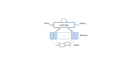
Figure 1: Graph Memory Network. At the first step, the controller reads the query; the memory is initialized by the input graph, one node embedding per memory cell. Then during the reasoning process, the controller iteratively reads from and writes to the memory. Finally, the controller computes the output.

GraphMem (Fig. 1) consists of a controller and an external memory, both of which, when rolled out, are recurrent neural networks (RNNs) interacting with each other. Different from the standard RNNs, the memory is a matrix RNN [31], where the hidden states are matrices with a graph imposed on columns. The controller first takes the query as the input and repeatedly reads from the memory using an attention mechanism, processes and sends the signals back to the memory cells. Each memory cell is first initialized by the input graph embedding, one node per cell. Then at each reasoning step, the cell content is updated by the signals from the controller and its neighbor memory cells in the previous step. Through multiple steps of reasoning, the memory cells are evolved from the original input to a refined stage, preparing the controller for generating the output. The query setting is flexible as it has been demonstrated in question-answering tasks [20].

The controller and attentive reading

Let $\boldsymbol{q}$ be the query vector and $\boldsymbol{h}_{t}$ be the state of the controller at time $t$ $\left(t=0,...,T\right)$. First, the controller reads the query: $\boldsymbol{h}_{0}=g\left(W_{q}\boldsymbol{q}\right)$. All biases are omitted for clarity.

During the multi-hop reasoning process to answer the query, the controller reads the summation vector $\boldsymbol{m}_{t}$ from the memory and updates its state as follows:

$$\boldsymbol{h}_{t}=g\left(W_{h}\boldsymbol{h}_{t-1}+U_{h}\boldsymbol{m}_{t}\right)$$ (1)

As $\boldsymbol{m}_{t}$ is the summation of the memory, the representation of the whole graph is embedded in $\boldsymbol{m}_{t}$, thus embedded in the controller $\boldsymbol{h}_{t}$. The hidden state of the controller contains both the graph and the query representations, which are neccessary to produce an output. The controller predicts an output after $T$ steps of the process of reasoning and updating. The output can be of any type corresponding to the query. For example, the query-output pairs can be (if a graph has a specific property - binary output) and (what is the solubility of a molecule compound - continuous output).

To read the vector $\boldsymbol{m}_{t}$ from the memory, a content-based addressing scheme, also known as soft attention, is employed. At each time step $t$ $\left(t=1,...,T\right)$, $\boldsymbol{m}_{t}$ is a sum of all memory cells, weighted by the probability $p_{t}^{i}$, for each memory cell $i=1,...M$:

$$\boldsymbol{a}_{t}^{i} = \text{tanh}\left(W_{a}\boldsymbol{m}_{t-1}^{i}+U_{a}\boldsymbol{h}_{t-1}\right)$$

$$p_{t}^{i} = \text{softmax}\left(\boldsymbol{v}^{\top}\boldsymbol{a}_{t}^{i}\right)$$

$$\boldsymbol{m}_{t} = \sum_{i}p_{t}^{i}\boldsymbol{m}_{t-1}^{i}$$

where $\boldsymbol{a}_{t}^{i}$ integrates information stored in the memory cell $\boldsymbol{m}_{t-1}^{i}$ and the controller state $\boldsymbol{h}_{t-1}$, and $\boldsymbol{v}$ is a parameter vector used to measure the contribution of memory cells to the summation vector. With this attention mechanism, the controller can selectively choose important nodes toward the query and the predictive output, rather than considering them equally. The query acts like an attention signal that guide the controller where to put more weight on.

Graph-structured Multi-relational Memory

The memory is extended from the unstructured memory in the E2E MemNet to a graph-structured multi-relational one. Each node in the graph $a^{i}$ has a feature vector (either extracted from the data, or through embedding) $\boldsymbol{x}^{i}\in\mathbb{R}^{K_{x}}$ ($i=1...M)$. The memory consists of $M$ memory cells, each cell $\boldsymbol{m}_{t}^{i}\in\mathbb{R}^{K_{m}}$ stores the information of the node $a^{i}$. The memory cells are initialized by a transformation of the feature vectors: $\boldsymbol{m}_{1}^{i}=g\left(\boldsymbol{x}^{i}\right)$. The memory cells connect to each other based on the node connections in the graph. If two nodes are connected through a relation, their corresponding memory cells have a connection. This enables the memory cells to embed the substructures of the graph by updating their content by the information from their neighbors.

At step $t$, each memory cell is updated by a function of the previous memory, a write content from the controller and the memories from the neighboring cells: $\boldsymbol{m}_{t}^{i}=f\left(\boldsymbol{m}_{t-1}^{i},\boldsymbol{h}_{t},\left(\boldsymbol{m}_{t-1}^{j}\right)_{j\in\mathcal{N}(i)}\right)$. In our experiments, the implementation of the memory update is as follow:

$$\boldsymbol{m}_{t}^{i} = g\left(W_{m}\boldsymbol{m}_{t-1}^{i}+U_{m}\boldsymbol{h}_{t}+\sum_{r}V_{r}\boldsymbol{c}_{tr}^{i}\right)$$ (2)

$$\boldsymbol{c}_{tr}^{i} = \sum_{j\in\mathcal{N}_{r}(i)}p^{j}\left[\boldsymbol{m}_{t-1}^{j},\boldsymbol{b}^{ij}\right]$$ (3)

where $\mathcal{N}_{r}(i)$ is the neighbor of the node $a^{i}$ with the relation type $r$ and $\boldsymbol{c}_{tr}^{i}$ denotes the neighboring context of relation $r$. $\left[\boldsymbol{m}_{t-1}^{j},\boldsymbol{b}^{ij}\right]$ is the concatenation of the memory cell $\boldsymbol{m}_{t-1}^{j}$ and the link feature vector $\boldsymbol{b}^{ij}$. $p^{j}$ is the weight of the node $a^{j}$, which indicates how important the node $a^{j}$ toward $a^{i}$ and $\sum_{j\in\mathcal{N}_{r}(i)}p^{j}=1$. $p^{j}$ can be learned similar to the memory cell probabilities in the attentive reading or can be pre-computed.

This update allows each memory cell to embed the neighbor information in its representation, thus, capturing the graph structure information. The neighboring update can be found in different graph-based neural networks [9, 32, 11]. The common idea is that each node can embed the graph substructure information around it by iteratively updating signals from its neighbors through multiple steps. For example, we have ($a^{1}$, $a^{2}$) and ($a^{2}$, $a^{3}$) are two connections. At first, the memory cell $\boldsymbol{m}_{1}^{1}$ contains the signals from $a^{2}$ and $\boldsymbol{m}_{1}^{2}$ contains the signals from $a^{3}$. At the second step, $\boldsymbol{m}_{2}^{1}$ updates signals from $\boldsymbol{m}_{1}^{2}$, which already contains information of $a^{3}$. If the number of steps is large enough, a node can contain information of the whole graph.

Recurrent skip-connections

The controller can be implemented in several ways. It could be a feedforward network or a recurrent network such as LSTM. In case of feedforward net, the query information is propagated through the memory via memory update. In case of recurrent nets, the query information is also propagated through the internal state of the controller. For simplicity, in this paper, we implement the controller and the memory updates using skip-connections [33, 34]

$$\boldsymbol{z}_{t}=\boldsymbol{\alpha}*\tilde{\boldsymbol{z}}_{t}+\left(1-\boldsymbol{\alpha}\right)*\boldsymbol{z}_{t-1}$$

where $\boldsymbol{\alpha}$ is a sigmoid gate moderating the amount of information flowing from the previous step, $\boldsymbol{z}_{t-1}$ is the state from the previous step and $\tilde{\boldsymbol{z}}_{t}$ is a proposal of the new state which is typically implemented as a nonlinear function of $\boldsymbol{z}_{t-1}$.

The controller $\boldsymbol{h}_{t}$ and the memory cell $\boldsymbol{m}_{t}^{i}$ are updated in a fashion similar to that of $\boldsymbol{z}_{t}$ while $\tilde{\boldsymbol{h}}_{t}$ and $\tilde{\boldsymbol{m}}_{t}^{i}$ are computed as in Eq. (1 and 2). This makes the memory cell update similar to the one in Differential Neural Computer [35], where the memory cells are partially erased and updated with new information.

Remark: With this choice of recurrence, the entire network can be considered as $M+1$ RNNs interacting following the structure defined by the multi-relational graph.

GraphMem for multi-task learning

GraphMem can be easily applied for multi-task learning. Suppose that the dataset contains $n$ tasks, each task is a set of graphs toward a specific type of output. We can use the query to indicate the task. If a graph is from task $k$, the query for the graph is a one-hot vector of size $n$: $\boldsymbol{q}=[0,0,...,1,0,...]$, where $\boldsymbol{q}^{k}=1$ and $\boldsymbol{q}^{j}=0$ for $j=1,...,n,\text{ }j\neq k$. The task index now becomes the input signal for GraphMem. With the signal from the task-specific query, the attention can identify which substructure is important for a specific task to attend on.

IV Experiments and Results

IV-A Datasets

We conducted experiments on 9 NCI BioAssay activity tests collected from the PubChem website . 7 of them are activity tests of chemical compounds against different types of cancer: breast, colon, leukemia, lung, melanoma, central nerve system and renal. The others are AIDS antiviral assay and Yeast anticancer drug screen. Each BioAssay test contains records of activities for chemical compounds. We chose the 2 most common activities for classification: “active” and “inactive”. Each compound molecule is represented as a graph, where nodes are atoms and edges are bonds between them. The statistics of data is reported in Table I. The datasets are listed by the ascending order of number of active compounds. “# Graph” is the number of graphs and “# Active” is the number of active graph against a BioAssay test These datasets are unbalanced, therefore “inactive” compounds are randomly removed so that the Yeast Anticancer dataset has 25,000 graphs and each of the other datasets has 10,000 graphs.

Table I: Summary of 9 NCI BioAssay datasets.

No.	Dataset	# Active	# Graph
1	AIDS Antiviral	1513	41,595
2	Renal Cancer	2,325	41,560
3	Central Nervous System	2,430	42,473
4	Breast Cancer	2,490	29,117
5	Melanoma	2,767	39,737
6	Colon Cancer	2,766	42,130
7	Lung Cancer	3,026	38,588
8	Leukemia	3,681	38,933
9	Yeast Anticancer	10,090	86,130

Fingerprint feature extraction

Fingerprints are the encoding of the graph structure of the molecules by a vector of binary digits, each presents the presence or absence of particular substructures in the molecules. There are different algorithms to achieve molecular fingerprints and the state of the art is the extended-connectivity circular fingerprint (ECFP) [36]. We use the RDKit toolkit to extraction circular fingerprints. The dimension of the fingerprint features is set by 1024.

Graph extraction

We also use RDKit to extract the structure of molecules, the atom and the bond features. An atom feature vector is the concatenation of the one-hot vector of the atom and other features such as atom degree and number of H atoms attached. We also make use of bond features such as bond type and a binary value indicating if a bond in a ring.

IV-B Experiment settings

To evaluate the benefit of multi-task learning, we trained the 9 datatasets separately and jointly on both fingerprint features and graph structure. In the multi-task setting, each dataset is a single task.

In the separated training setting, three common classifiers: Support Vector Machine (SVM), Random Forest (RF) and Gradient Boosting Machine (GMB) are trained on fingerprint features, and Neural Fingerprint (NeuralFP) [12] and our GraphMem are trained on graph structure. The query of GraphMem for each dataset is set by a constant vector.

In the joint training setting, we trained Multitask Neural Network (MT-NN) [18] on fingerprint features and our model (MT-GraphMem) on graph structure. The query for a molecule of task $i$ is a one-hot vector $\boldsymbol{q}\in\mathbb{R}^{K}$, where $K$ is the number of tasks, $\boldsymbol{q}^{i}=1$ and $\boldsymbol{q}^{j}=0$ for all $j\neq i$. For simplicity, we set the weights in Eq. 3 uniformly.

For training neural networks, the training minimizes the cross-entropy loss in an end-to-end fashion. We use ReLU units for all steps and Dropout [37] is applied at the first and the last steps of the controller and the memory cells. We set the number of hops by $T=10$ and other hyper-parameters are tuned on the validation dataset.

IV-C The impact of more datasets

We evaluate how performance of GraphMem on a particular dataset is affected by the increasing number of tasks. We chose AIDS antiviral, Breast Cancer and Colon Cancer as the experimental datasets. For each experimental dataset, we start to train it and then repeatedly add a new task and retrain the model. The orders of the first three new tasks are: (AIDS, Breast, Colon) for AIDS antiviral dataset, (Breast, AIDS, Colon) for Breast Cancer dataset and (Colon, AIDS, Breast) for Colon Cancer dataset. The orders of the remaining tasks are the same for 3 datasets: (Leukemia, Lung, Melanoma, Nerve, Renal and Yeast).

Fig. 2 illustrates the performance of the three chosen datasets with different number of jointly training tasks. The performance of Breast and Colon Cancer datasets decreases when jointly trained with AIDS antiviral task and then increases after adding more tasks and remain steady or slightly reduce after 7 tasks. Jointly training does not really improve the performance on the AIDS antiviral dataset.

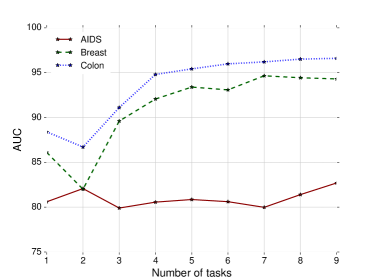
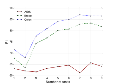
(a)	(b)

Figure 2: The performance of three datasets when increasing the number of jointly training tasks, reported in (a) AUC and (b) F1-score.

IV-D Results

Table II: Performance over all datasets, measured in Micro F1, Macro F1 and the average AUC.

Model	MicroF1	MacroF1	Average AUC
SVM	66.4	67.9	85.1
RF	65.6	66.4	84.7
GB	65.8	66.9	83.7
NeuralFP [12]	68.2	67.6	85.9
GraphMem	69.1	68.7	85.9
MT-NN [18]	75.5	78.6	90.4
MT-GraphMem	77.8	80.3	92.1

Table II reports results, measured in Micro F1-score, Macro F1-score and the average AUC over all datasets. The best method for separated training on fingerprint features is SVM with 66.4% of Micro F1-score and on graph structure is GraphMem with the improvement of 2.7% over the non-structured classifiers. The joint learning settings improve a huge gap with 9.1% of Micro F1-score and 10.7 % of Macro F1-score gain on fingerprint features and 8.7% of Micro F1-score and 11.6% of Macro F1-score gain on graph structure.

To investigate more on how multi-task learning impacts the performance of each task, we reports the F1-score of GraphMem in both separately and jointly training settings on each of the 9 datasets (Fig. 3). Joint training with GraphMem model does not improve the performance on AIDS antiviral and Yeast anticancer datasets while for 7 datasets on different types of cancers, joint training improves the performance from 10%-20% on each task.

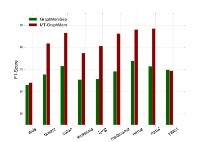
Figure 3: The comparison in performance of GraphMem when training separately (GraphMemSep) and jointly (MT-GraphMem) for all datasets. Best view in color.

V Discussion

We have proposed Graph Memory Network (GraphMem), a neural network augmented with a dynamic and graph-structured memory and applied it for modeling molecules. Experiments on 9 BioAssay activity tests demonstrated that GraphMem is effective in answering queries about bioactivities of large molecules given only the molecular graphs. We applied the model for multi-task learning with the query indicating the task number. However, the query is very flexible, it can be any question about the property of a molecule.

There is room for further investigations. First, we wish to emphasize that GraphMem is a general models for answering any query about graph data. This opens up new applied opportunities in other domains, for example, textual and visual question answering about interacting actors and objects. Second, BioAssay activity ground truths used in training for each target (e.g., a disease) are expensive to establish. We can leverage the strength of statistics from the existing large datasets to improve over the smaller datasets. For example, each BioAssay test can be considered as a task and the model can jointly learn all tasks. The task ID and other information of the molecule can be embedded in the query. Furthermore, the memory structure in GraphMem, once constructed from data graphs, is then fixed even though the content of the memory changes during the reasoning process. A future work would be deriving dynamic memory graphs that evolve with time.

References

- [1] A. Cherkasov, E. N. Muratov, D. Fourches, A. Varnek, I. I. Baskin, M. Cronin, J. Dearden, P. Gramatica, Y. C. Martin, R. Todeschini et al., “QSAR modeling: where have you been? Where are you going to?” Journal of medicinal chemistry, vol. 57, no. 12, pp. 4977–5010, 2014.
- [2] R. Burbidge, M. Trotter, B. Buxton, and S. Holden, “Drug design by machine learning: support vector machines for pharmaceutical data analysis,” Computers & chemistry, vol. 26, no. 1, pp. 5–14, 2001.
- [3] R. N. Jorissen and M. K. Gilson, “Virtual screening of molecular databases using a support vector machine,” Journal of chemical information and modeling, vol. 45, no. 3, pp. 549–561, 2005.
- [4] V. Svetnik, A. Liaw, C. Tong, J. C. Culberson, R. P. Sheridan, and B. P. Feuston, “Random forest: a classification and regression tool for compound classification and qsar modeling,” Journal of chemical information and computer sciences, vol. 43, no. 6, pp. 1947–1958, 2003.
- [5] V. Svetnik, T. Wang, C. Tong, A. Liaw, R. P. Sheridan, and Q. Song, “Boosting: An ensemble learning tool for compound classification and qsar modeling,” Journal of chemical information and modeling, vol. 45, no. 3, pp. 786–799, 2005.
- [6] Y. LeCun, Y. Bengio, and G. Hinton, “Deep learning,” Nature, vol. 521, no. 7553, pp. 436–444, 2015.
- [7] I. I. Baskin, D. Winkler, and I. V. Tetko, “A renaissance of neural networks in drug discovery,” Expert opinion on drug discovery, vol. 11, no. 8, pp. 785–795, 2016.
- [8] G. E. Dahl, N. Jaitly, and R. Salakhutdinov, “Multi-task neural networks for qsar predictions,” arXiv preprint arXiv:1406.1231, 2014.
- [9] F. Scarselli, M. Gori, A. C. Tsoi, M. Hagenbuchner, and G. Monfardini, “The graph neural network model,” IEEE Transactions on Neural Networks, vol. 20, no. 1, pp. 61–80, 2009.
- [10] J. Atwood and D. Towsley, “Diffusion-convolutional neural networks,” in Advances in Neural Information Processing Systems, 2016, pp. 1993–2001.
- [11] T. Pham, T. Tran, D. Phung, and S. Venkatesh, “Column networks for collective classification,” AAAI, 2017.
- [12] D. K. Duvenaud, D. Maclaurin, J. Iparraguirre, R. Bombarell, T. Hirzel, A. Aspuru-Guzik, and R. P. Adams, “Convolutional networks on graphs for learning molecular fingerprints,” in Advances in neural information processing systems, 2015, pp. 2224–2232.
- [13] S. Kearnes, K. McCloskey, M. Berndl, V. Pande, and P. Riley, “Molecular graph convolutions: moving beyond fingerprints,” Journal of computer-aided molecular design, vol. 30, no. 8, pp. 595–608, 2016.
- [14] J. Gilmer, S. S. Schoenholz, P. F. Riley, O. Vinyals, and G. E. Dahl, “Neural message passing for quantum chemistry,” ICML, 2017.
- [15] Q. V. Le and T. Mikolov, “Distributed representations of sentences and documents,” ICML, 2014.
- [16] S. V. N. Vishwanathan, N. N. Schraudolph, R. Kondor, and K. M. Borgwardt, “Graph kernels,” Journal of Machine Learning Research, vol. 11, no. Apr, pp. 1201–1242, 2010.
- [17] M. Choetkiertikul, H. K. Dam, T. Tran, A. Ghose, and J. Grundy, “Predicting delivery capability in iterative software development,” IEEE Transactions on Software Engineering, 2017.
- [18] B. Ramsundar, S. Kearnes, P. Riley, D. Webster, D. Konerding, and V. Pande, “Massively multitask networks for drug discovery,” arXiv preprint arXiv:1502.02072, 2015.
- [19] T. Unterthiner, A. Mayr, G. Klambauer, and S. Hochreiter, “Toxicity prediction using deep learning,” arXiv preprint arXiv:1503.01445, 2015.
- [20] S. Sukhbaatar, A. Szlam, J. Weston, and R. Fergus, “End-to-end memory networks,” NIPS, 2015.
- [21] A. Graves, G. Wayne, and I. Danihelka, “Neural turing machines,” arXiv preprint arXiv:1410.5401, 2014.
- [22] E. Parisotto and R. Salakhutdinov, “Neural map: Structured memory for deep reinforcement learning,” arXiv preprint arXiv:1702.08360, 2017.
- [23] T. Bansal, A. Neelakantan, and A. McCallum, “RelNet: End-to-end Modeling of Entities & Relations,” arXiv preprint arXiv:1706.07179, 2017.
- [24] M. M. Bronstein, J. Bruna, Y. LeCun, A. Szlam, and P. Vandergheynst, “Geometric deep learning: going beyond euclidean data,” arXiv preprint arXiv:1611.08097, 2016.
- [25] J. Bruna, W. Zaremba, A. Szlam, and Y. LeCun, “Spectral networks and deep locally connected networks on graphs,” in ICLR, 2014.
- [26] M. Henaff, J. Bruna, and Y. LeCun, “Deep convolutional networks on graph-structured data,” arXiv preprint arXiv:1506.05163, 2015.
- [27] D. D. Johnson, “Learning graphical state transitions,” ICLR, 2017.
- [28] Y. Li, D. Tarlow, M. Brockschmidt, and R. Zemel, “Gated graph sequence neural networks,” ICLR, 2016.
- [29] M. Niepert, M. Ahmed, and K. Kutzkov, “Learning convolutional neural networks for graphs,” in Proceedings of the 33rd annual international conference on machine learning. ACM, 2016.
- [30] M. Schlichtkrull, T. N. Kipf, P. Bloem, R. v. d. Berg, I. Titov, and M. Welling, “Modeling relational data with graph convolutional networks,” arXiv preprint arXiv:1703.06103, 2017.
- [31] K. Do, T. Tran, and S. Venkatesh, “Learning recurrent matrix representation,” Third Representation Learning for Graphs Workshop (ReLiG 2017), 2017.
- [32] Y. Li, D. Tarlow, M. Brockschmidt, and R. Zemel, “Gated graph sequence neural networks,” arXiv preprint arXiv:1511.05493, 2015.
- [33] T. Pham, T. Tran, D. Phung, and S. Venkatesh, “Faster training of very deep networks via p-norm gates,” ICPR, 2016.
- [34] R. K. Srivastava, K. Greff, and J. Schmidhuber, “Training very deep networks,” in Advances in neural information processing systems, 2015, pp. 2377–2385.
- [35] A. Graves, G. Wayne, M. Reynolds, T. Harley, I. Danihelka, A. Grabska-Barwińska, S. G. Colmenarejo, E. Grefenstette, T. Ramalho, J. Agapiou et al., “Hybrid computing using a neural network with dynamic external memory,” Nature, vol. 538, no. 7626, pp. 471–476, 2016.
- [36] D. Rogers and M. Hahn, “Extended-connectivity fingerprints,” Journal of chemical information and modeling, vol. 50, no. 5, pp. 742–754, 2010.
- [37] N. Srivastava, G. Hinton, A. Krizhevsky, I. Sutskever, and R. Salakhutdinov, “Dropout: A simple way to prevent neural networks from overfitting,” Journal of Machine Learning Research, vol. 15, pp. 1929–1958, 2014.