CPHT-RR102.122017

Corrections in the relative entropy of black hole microstates

Ben Michel${}^{\includegraphics[scale={0.07}]{calib.pdf}}{}^{\includegraphics[scale={0.0139}]{caliw.pdf}}$ and Andrea Puhm${}^{\blacklozenge}{}^{\diamondsuit}{}^{\odot}$

${}^{\includegraphics[scale={0.07}]{calib.pdf}}$ Mani L. Bhaumik Institute for Theoretical Physics

Department of Physics and Astronomy, University of California

Los Angeles, CA 90095

${}^{\includegraphics[scale={0.0139}]{caliw.pdf}}$ Department of Physics, University of California

Santa Barbara, CA 93106

^◆ CPHT, École Polytechnique, CNRS

91128, Palaiseau, France

^♢ Jefferson Physical Laboratory, Harvard University

Cambridge, MA 02138

^⊙ Black Hole Initiative, Harvard University

Cambridge, MA 02138

Inspired by the recent work of Bao and Ooguri (BO), we study the distinguishability of the black hole microstates from the thermal state as captured by the average of their relative entropies: the Holevo information. Under the assumption that the vacuum conformal block dominates the entropy calculation, BO find that the average relative entropy vanishes on spatial regions smaller than half the size of the CFT. However, vacuum block dominance fails for some microstates of the $M=0$ BTZ black hole. We show that this renders the average relative entropy nonzero even on infinitesimal intervals at $O(c^{0})$.

1 Introduction

Relative entropy is among the most powerful tools available for characterizing the distinguishability of two quantum states, and has recently found broad application in holography: its equality on bulk and boundary convincingly identifies the entanglement wedge as the dual to a given boundary region [1]; its positivity and monotonicity leads to proofs of the average null energy condition [2] and the generalized second law [3]; its expansion about the vacuum leads to a derivation of Einstein’s equations from the dynamics of entanglement [4, 5, 6, 7, 8, 9]. One might hope to use relative entropy to further probe questions related to the black hole information paradox, such as how easily the black hole microstates can be distinguished from the coarse-grained thermal state of the black hole.

Unfortunately, despite our ability to make general statements about its properties, relative entropy is not an easy quantity to compute in black hole microstates. Unlike its less-useful cousins – the entanglement and Renyi entropies – it lacks a simple replica expression as a four-point function, and instead requires calculation of $n$-point correlators of heavy operators [10, 11].

Bao and Ooguri [12] have recently identified an analog quantity which can be more easily computed – the Holevo information $\chi$. Given an ensemble $\rho=\sum_{i}p_{i}\rho_{i}$ of density matrices $\rho_{i}$, the Holevo information is the average entropy of the $\rho_{i}$ relative to $\rho$:

$$\chi(\rho) =\sum_{i}p_{i}S(\rho_{i}||\rho)$$

$$=S(\rho)-\sum_{i}p_{i}S(\rho_{i})\,.$$ (1.1)

Here the $\rho_{i}$ and $\rho$ are normalized density matrices, the $p_{i}$ form a normalized probability distribution, and in the second line we used the definition of relative entropy:

$$S(\sigma||\rho)=-\text{tr}(\sigma\log\rho)+\text{tr}(\sigma\log\sigma).$$ (1.2)

Since the average relative entropy $\chi$ is equal to the average difference in von Neumann entropy between $\rho$ and the $\rho_{i}$, computation of $\chi$ reduces to the computation of tractable (heavy-light) four-point functions.

Bao and Ooguri estimated this quantity for the thermal density matrix of a black hole in anti-de Sitter space at temperature $1/\beta$:

$$\rho_{\text{BH}}=Z^{-1}\sum_{i}e^{-\beta E_{i}}\left|E_{i}\right>\left<E_{i}\right|.$$ (1.3)

Here the microstates $\rho_{i}$ are the energy eigenstates $\left|E_{i}\right>\left<E_{i}\right|$ weighted by a Boltzmann factor $p_{i}\propto e^{-\beta E_{i}}$. They can be perfectly distinguished by an observer who has access to the entire dual CFT, but a less omniscient observer has a more difficult task.

Within a ball-shaped subregion $A_{\ell}$ of the CFT with diameter $\ell$, average distinguishability is characterized by the Holevo information of the reduced density matrix $\rho_{\ell}$ obtained by tracing over the complement of the region:

$$\rho_{\ell}\equiv\text{tr}_{{\bar{A}_{\ell}}}\rho.$$ (1.4)

In general dimension there is no known way to compute the $S(\rho_{\ell})$ in field theory and so one must resort to holographic arguments, using the HRRT [13, 14] formula in either the black hole background or the (generically unknown) background created by a heavy operator. However, in large-$c$ CFTs the vacuum block contribution to the heavy-heavy-light-light four-point function can be computed using the bootstrap [15], which in turn makes it possible to compute $S(\rho_{i,\ell})$ in CFT [16] if one makes the assumption that conformal blocks other than the vacuum do not contribute. Bao and Ooguri use this approximation to obtain [12]

$$\chi(\rho_{\text{BH},\ell})\approx\left\{\begin{array}[]{ll}0&\ell\leq\pi R\\ \frac{c}{3}{\rm log}\left[\frac{\sinh(\pi\ell/\beta)}{\sinh\left(\pi(2\pi R-\ell)/\beta\right)}\right]&\pi R<\ell<\ell_{crit}\\ S_{BH}&\ell\geq\ell_{crit}\,,\end{array}\right.$$ (1.5)

where $c$ is the central charge of the CFT and $\ell_{crit}$ is a critical length that follows from the homology constraint in the Ryu-Takayanagi formula. We have reintroduced the radius $R$ of the spatial circle of the CFT and corrected several factors in this expression.

The vacuum block does not dominate at subleading orders in $1/c$ [17] and so one would naturally expect (1.5) to receive corrections. However, we will show that $1/c$ corrections to (1.5) are also induced by competition with the vacuum block in $S(\rho_{i,\ell})$ at leading order in certain states. This generates $1/c$ corrections to the average relative entropy once the rarity of these states is taken into account.

We will study these corrections in the $\beta\rightarrow\infty$ limit corresponding to the $M=0$ BTZ black hole [18, 19], which has a microscopic description in terms of D-branes whose near-horizon geometry is AdS${}_{3}\times S^{3}$ [20] (the $S^{3}$ is necessary in the microscopic formulation of the theory and will play an important role). We restrict to infinitesimal intervals $\ell\rightarrow 0$ in the CFT, where the structure of entanglement entropy can be made particularly explicit [21, 22]. The correction to $\chi$ that we estimate comes from states $\left|i\right>$ whose R-charges $J$ scale with $c$, corresponding to gravitational solutions with angular momentum on the $S^{3}$. The expectation values $\langle J\rangle_{i}$ grow with the central charge, violating the assumption of vacuum block dominance.

Our main result is an $O(c^{0})$ correction to the average relative entropy in the small interval limit $\ell\rightarrow 0$:

$$\boxed{\chi(\rho_{\text{BH},\ell})=\alpha\left(\frac{\ell}{R}\right)^{2}+\dots}$$ (1.6)

where $\alpha$ is an $O(c^{0})$ coefficient. The ellipses denote further positive corrections: at $O(\ell^{2})$ from BPS operators other than $J$ with conformal weights $h+\bar{h}=1$, and at higher orders in $\ell$ from higher-dimension operators. We also resolve the minor discrepancy between the holographic and field-theoretic computations of [22].

The rest of this note is organized as follows. In § 2 we briefly review the work of Bao and Ooguri and their input assumptions. In § 3 we review the work of Giusto and Russo on entanglement entropy in black hole microstates, which leads to our main result. We conclude in § 4 with some broader context. In the appendix we give two derivations of the density of states at generic R-charges: the first is intuitive and can be visualized; the second, which extends the thermodynamic analysis of Balasubramanian et al [23], allows us to systematically compute finite-$N$ corrections.

2 Review of the Bao-Ooguri Estimate

In the AdS₃/CFT₂ correspondence the BTZ black hole is dual to the thermal ensemble (1.3). Following [12], we will be interested in characterizing the distinguishability of the microstates $\rho_{i}$ from the ensemble (1.3) on an interval of length $\ell$ in the CFT, which we take to live on a circle of radius $R$. It is captured by the relative entropy

$$S(\rho_{i,\ell}||\rho_{\text{BH},\ell})=-{\rm tr}(\rho_{i,\ell}{\rm log}\,\rho_{\text{BH},\ell})+{\rm tr}(\rho_{i,\ell}{\rm log}\,\rho_{i,\ell})\,,$$ (2.1)

where $\rho_{i,\ell}$ and $\rho_{\text{BH},\ell}$ are the reduced density matrices defined in (1.4). The average of this quantity – the Holevo information – is equal to the average difference of von Neumann entropies:

$$\chi(\rho_{\text{BH},\ell}) =\sum_{i}p_{i}S(\rho_{i,\ell}||\rho_{\text{BH},\ell})$$

$$=S(\rho_{\text{BH},\ell})-\sum_{i}p_{i}S(\rho_{i,\ell})\,.$$ (2.2)

It was recently argued [12] that the Holevo information is zero on intervals smaller than half of the circle, $\ell<\pi R$. We will argue in the next section that $1/c$ corrections make the Holevo information nonzero even on infinitesimal intervals but first, we review the arguments of [12], highlighting the assumption that will be violated in our scenario.

In order to evalute (2) one needs the von Neumann entropies of the reduced density matrices. When the CFT is holographic, these entropies are determined by the HRRT formula [13, 14],

$$S_{RT}(\rho_{\ell})=\frac{{\rm length}(\Gamma_{\ell})}{4G}\,.$$ (2.3)

Here $\Gamma_{\ell}$ is the extremal surface in the bulk dual of $\rho$, homologous to the boundary region $A_{\ell}$.

When $\rho=\rho_{\text{BH}}$ the dual geometry is the BTZ black hole. The homology constraint then implies a critical length $\ell_{crit}$ where the extremal surface splits into two disconnected pieces, one wrapping the black hole and another homologous to the complementary region:

$$S(\rho_{\text{BH},\ell})=\left\{\begin{array}[]{ll}S_{RT}(\rho_{\text{BH},\ell})&\quad\ell<\ell_{crit}\\ S_{RT}(\rho_{\text{BH},2\pi R-\ell})+S_{BH}&\quad\ell\geq\ell_{crit}.\end{array}\right.$$ (2.4)

The bulk dual of a generic microstate is not known, but one can still study the $S(\rho_{i,\ell})$ using field-theoretic methods. Bao and Ooguri [12] estimated the microstate entropies using the results of [16], which starts from the replica trick for entanglement entropy in 1+1d CFTs [24]:

$$S(\rho_{i,\ell})=-{\rm tr}\,\rho_{i,\ell}{\rm log}\,\rho_{i,\ell}=\lim_{n\to 1}\frac{1}{1-n}{\rm log}\left[\mathcal{Z}^{-1}\langle\Psi_{i}(\infty)\mathcal{T}_{n}(u,\bar{u}){\mathcal{T}}_{-n}(v,\bar{v})\Psi_{i}(0)\rangle\,\right]\,.$$ (2.5)

Here $u$ and $v$ are the endpoints of the interval, $\left|\Psi_{i}\right>=\left|i\right>^{\otimes n}$, the $\mathcal{T}_{n}$ are twist operators with weights $h_{\mathcal{T}}=\bar{h}_{\mathcal{T}}=\frac{c}{24}\frac{n^{2}-1}{n}$, and we have made explicit the renormalization factor $\mathcal{Z}$.

The four-point function in (2.5) can be expanded in conformal blocks [16], using a scale transformation to move the operators to $(0,1,x,\infty)$:

$$\langle\Psi_{i}(\infty)\mathcal{T}_{n}(x,\bar{x}){\mathcal{T}}_{-n}(1)\Psi_{i}(0)\rangle=\sum_{\mathcal{O}_{p}}a_{p}^{(i)}\,\mathcal{F}(nc;nh_{i},h_{\mathcal{T}},h_{p};1-x)\bar{\mathcal{F}}(nc;n\bar{h}_{i},\bar{h}_{\mathcal{T}},\bar{h}_{p};1-\bar{x})\,.$$ (2.6)

Here the sum runs over Virasoro primaries, $a_{p}^{(i)}=C_{iip}C_{\mathcal{T}{\mathcal{T}}}^{p}$, and $x=u/v$ is the conformal cross-ratio. We have chosen to expand in the $t$-channel to anticipate our eventual interest in the small-interval limit.

In large-$c$ conformal field theories this expression can be evaluated at leading order in $c$ under the additional assumption of vacuum block dominance [25], i.e. that the sum is well-approximated by the contribution of the identity and its descendants:

$$\lim_{c\rightarrow\infty}\,\langle\Psi_{i}(\infty)\mathcal{T}_{n}(x,\bar{x}){\mathcal{T}}_{-n}(1)\Psi_{i}(0)\rangle\stackrel{{\scriptstyle?}}{{\approx}}\mathcal{F}(nc;nh_{i},h_{\mathcal{T}},0;1-x)\bar{\mathcal{F}}(nc;n\bar{h}_{i},\bar{h}_{\mathcal{T}},0;1-\bar{x})\,.$$ (2.7)

This approximation is valid (in some range of $x$) only in states where $a_{p}^{(i)}$ grows slowly with $c$ for all light primaries $\mathcal{O}_{p}$ [25, 16]. In the next section we consider a class of black hole microstates that violate this condition and discuss their impact on $\chi$.

If one simply assumes vacuum block dominance, the correlator in (2.5) can be computed in the limit $n\rightarrow 1$ [16] using the known form of the heavy-heavy-light-light vacuum block [15] in the channel in which it dominates. The result is the vacuum block contribution to $S(\rho_{i,\ell})$:

$$S(\rho_{i,\ell})|_{\text{vac}}=\frac{c}{3}{\rm log}\left[\frac{\beta_{i}}{\pi\,\epsilon}\sinh\left(\frac{\pi\,{\rm min}(\ell,2\pi R-\ell)}{\beta_{i}}\right)\right]\,,$$ (2.8)

where

$$\beta_{i}=\frac{2\pi}{\sqrt{24h_{i}/c-1}}$$ (2.9)

and $\epsilon$ is the UV cutoff. When $\ell>\pi R$ the vacuum block dominates in the channel obtained by replacing $\ell$ with $2\pi R-\ell$ [16], leading to the min in (2.8). This is the expression that is used in [12] to obtain the estimate (1.5), with the weight $h_{i}$ of the microstate fixed by demanding $\beta_{i}=\beta$. It agrees precisely with the holographic entropy (2.3) in the BTZ geometry if one relaxes the homology constraint [16].

Collecting (2.4) and (2.8), the vacuum block contribution to $\chi$ is

$$\chi(\rho_{\text{BH},\ell})|_{\text{vac}}=\left\{\begin{array}[]{ll}0&\quad\ell<\pi R\\ S_{RT}(\rho_{\text{BH},\ell})-S_{RT}(\rho_{\text{BH},2\pi R-\ell})=\frac{c}{3}{\rm log}\left[\frac{\sinh(\pi\ell/\beta)}{\sinh\left(\pi(2\pi R-\ell)/\beta\right)}\right]&\quad\pi R\leq\ell\leq\ell_{crit}\\ S_{BH}&\quad\ell>\ell_{crit}.\end{array}\right.$$ (2.10)

We will see that the failure of vacuum block dominance makes $\chi\sim O(c^{0})$ even when $\ell\ll\pi R$.

3 Fuzziness and Distinguishability

3.1 Entanglement entropy in the $M=0$ BTZ microstates

We will study the Holevo information in a string theory setup where the microstates of the black hole can be identified explicitly: the near-horizon limit of the D1-D5 brane system, whose CFT description includes 1/4-BPS states that are dual to microstates of the $M=0$ BTZ black hole ($\times\,S^{3}\times\,M_{4}$). The study of these states and their identification with dual geometries [26] is a rich subject with a long and tempestuous history; we will not make use of this identification here. Our results follow solely from the properties of 1/4-BPS operators in the CFT and are independent of (but consistent with) the identification of certain BPS operators with bulk geometries. For more details of the CFT see e.g. [37, 26, 38, 23, 39] and references therein.

The field theory description of the microstates is obtained by considering type IIB string theory on $S^{1}\times M_{4}$ with $N_{1}$ D1s wrapping the $S^{1}$ and $N_{5}$ D5s wrapping all the compactified directions, with the closed string sector decoupled by the near-horizon limit. Taking $M_{4}$ much smaller than the $S^{1}$, the theory becomes a 1+1d SCFT with $\mathcal{N}=(4,4)$ SUSY, whose central charge $c=6N_{1}N_{5}\equiv 6N$ is determined by the number of D1 and D5 branes. At weak coupling the SCFT is conjectured to be a nonlinear sigma model on the symmetric product orbifold $(M_{4})^{N}/S_{N}$ [40]; at strong coupling it is dual to supergravity in AdS${}_{3}\times\,S^{3}\times\,M_{4}$ [41].

The microstates of the $M=0$ BTZ black hole correspond to the Ramond ground states of this D1-D5 CFT [42, 43]. Supersymmetry protects their dimensions and $SU(2)_{L}\times SU(2)_{R}$ R-charges, which can therefore be extrapolated from the orbifold theory to the region of moduli space where the theory has a gravitational dual. The R-charges of the black hole microstates are bounded by $-\frac{N}{2}<J^{3}_{L},J^{3}_{R}<\frac{N}{2}$ [36] and correspond to angular momenta on the $S^{3}$ in the bulk [44]. Most states have $J^{3}_{L/R}\gtrsim O(\sqrt{N})$, violating vacuum block dominance.

As in any CFT corrections to the vacuum entropy are particularly easy to isolate in the small-interval limit, where the physics is determined by the twist operator OPE [21]. Since $\mathcal{T}_{n}\mathcal{T}_{-n}$ has vanishing twist, only untwisted operators $\mathcal{O}=\mathcal{O}_{p_{1}}^{(1)}\otimes\dots\otimes\mathcal{O}_{p_{n}}^{(n)}$ appear:

$$\mathcal{T}_{n}(w,\bar{w})\mathcal{T}_{-n}(w^{\prime},\bar{w}^{\prime}) = \frac{1}{|w-w^{\prime}|^{4h_{\mathcal{T}}}}\Big{[}1+\sum_{p}\sum_{r=1}^{n}(w-w^{\prime})^{h_{p}}(\bar{w}-\bar{w}^{\prime})^{\bar{h}_{p}}C_{\mathcal{T}\mathcal{T}}^{p_{r}}\,\mathcal{O}_{p}^{(r)}$$

$$+\sum\limits_{\begin{subarray}{c}p,q\\ r\neq s\end{subarray}}(w-w^{\prime})^{h_{p}+h_{q}}(\bar{w}-\bar{w}^{\prime})^{\bar{h}_{p}+\bar{h}_{q}}C_{\mathcal{T}\mathcal{T}}^{(p_{r},q_{s})}\,\mathcal{O}_{p}^{(r)}\otimes\mathcal{O}_{q}^{(s)}+\dots\Big{]},$$

with further terms subleading as $w\rightarrow w^{\prime}$. Here $r,s$ are replica indices and the expansion has been organized according to how many of the tensor factors in $\mathcal{O}$ are trivial (e.g. on the second line the operator is $\mathcal{O}_{p}$ on the $r^{\text{th}}$ factor tensored with $\mathcal{O}_{q}$ on the ${s}^{\text{th}}$ factor, tensored with the identity on the remaining factors). This expansion was studied by [22] in the Ramond ground states dual to the microstates of the $M=0$ BTZ black hole; we review their treatment, amending two points.

In any state $\left|i\right>$, the entanglement entropy of a small interval can be computed by plugging (3.1) into (2.5). We use coordinates $w$ on the cylinder related to the plane coordinates $z$ via $z=e^{iw}$, with the parametrization

$$w=\frac{\phi}{R}+i\tau,\quad\quad\tau\in\mathbb{R},\quad\quad\phi\equiv\phi+2\pi R.$$ (3.2)

The operators in (3.1) are inserted at $\phi-\phi^{\prime}=\ell$ on a constant-$\tau$ slice.

As $\ell\rightarrow 0$ the dominant contributions to (3.1) come from the lightest operators in the theory. The leading correction naively appears to be the first non-vacuum term in (3.1), but this term vanishes for all primaries since $C_{\mathcal{T}\mathcal{T}p_{r}}=0$ if $\mathcal{O}_{p}$ is primary. In the $M=0$ BTZ microstates, the leading correction to the entropy comes from a sum over the lightest untwisted primaries with two tensor factors nontrivial. When these operators have nontrivial expectation values they will contribute to the entanglement entropy. The OPE coefficients $C_{\mathcal{T}\mathcal{T}}^{(p_{r},q_{s})}$ can be determined by computing the expectation value of $\mathcal{O}_{p}^{(r)}\otimes\mathcal{O}_{q}^{(s)}$ on the replica manifold via a conformal map [21], then using the inverse of the Zamolodchikov metric $\mathfrak{g}_{ab}=\langle O_{a}|O_{b}\rangle$ to raise the index [22].

We would like to compute the microstate entropies $S(\rho_{i,\ell})$ in the gravity regime, but the orbifold CFT is at zero coupling. Fortunately, there is strong evidence that the gravity computation of (3.1) can be extracted from the calculation in the orbifold theory. The idea is as follows [22]: most operators acquire $O(c)$ anomalous dimensions at strong coupling and so will contribute negligibly to (3.1). However, 1/4-BPS operators are protected by supersymmetry: their dimensions and three-point functions are independent of the coupling[45]. To extrapolate results from the orbifold theory to gravity we therefore keep only the contributions from these BPS operators (we will leave the 1/4 implicit for brevity). It was shown in [22] that this prescription agrees exactly with the results obtained from a generalization of the HRRT formula, apart from the vacuum piece we will correct.

The lightest BPS operators in the D1-D5 CFT have $h+\bar{h}=1$ and thus appear at $O(\ell^{2})$ in the twist OPE (3.1). Inserting (3.1) into the formula for the entropy (2.5) and evaluating the sum over $r$ and $s$ in this sector exactly as in [22], at $O(\ell^{2})$ we find

$$\left<\Psi_{i}\right|\mathcal{T}_{n}(w,\bar{w})\mathcal{T}_{-n}(w^{\prime},\bar{w}^{\prime})\left|\Psi_{i}\right>=\left(\frac{R}{\ell}\right)^{\frac{c}{6}\frac{n^{2}-1}{n}}\left[1+\sum_{p,q}\left(\frac{\ell}{R}\right)^{2}\,\frac{(n^{2}-1)}{24n}\,\mathcal{M}_{(p,q)}\,\langle\mathcal{O}_{p}\rangle_{i}\langle\mathcal{O}_{q}\rangle_{i}+\dots\right]$$ (3.3)

where $\mathcal{M}$ is the contraction of the Zamolodchikov metric with the plane two-point function:

$$\mathcal{M}_{(p,q)}=\mathfrak{g}^{\{(p,q),(p^{\prime},q^{\prime})\}}\left<0\right|\mathcal{O}_{p^{\prime}}(1)\mathcal{O}_{q^{\prime}}(0)\left|0\right>_{\text{plane}}.$$ (3.4)

Among the lightest BPS operators are the holomorphic and antiholomorphic $SU(2)_{L}\times SU(2)_{R}$ R-symmetry currents $J^{\alpha}_{L}$ and $J^{\alpha}_{R}$. For simplicity we will focus on corrections to the Holevo information coming from the $\alpha=3$ components alone, neglecting the rest of the lightest BPS operators; we will abbreviate $J^{3}_{L/R}\equiv J_{L/R}$. Our computation of these corrections will be enough to show that $\chi\gtrsim O(c^{0})$ at small $\ell$, since the other operators that contribute at $O(\ell^{2})$ make manifestly positive contributions to $\chi$.

To obtain $S(\rho_{i,\ell})$ from (3.3) we must include the renormalization factor $\mathcal{Z}$, which was omitted in [22]. In the theory on the plane, the renormalization factor $\mathcal{Z}_{\text{plane}}=\epsilon^{-4h_{\mathcal{T}}}$ is introduced in order to make the entropy dimensionless [24]. However, there is no need to fix the units in (3.3) and so it seems we are free to choose $\mathcal{Z}_{\text{cyl}}$ as we please. We will fix it here by demanding that the leading divergence in $S(\rho_{i,\ell})$ approaches the vacuum entropy on the plane when $\ell\ll R$. This scheme is natural in light of the conformal symmetry: we should get the same results regardless of whether we do the computation directly in the theory on the cylinder, or by transforming the four-point function on the plane normalized by $\mathcal{Z}_{\text{plane}}$. Thus we take

$$\mathcal{Z}_{\text{cyl}}=\left(\frac{\epsilon}{R}\right)^{-4h_{\mathcal{T}}}.$$ (3.5)

Taking $\mathcal{Z}_{\text{cyl}}$ into account, focusing just on the contribution of $J_{L/R}$ and following the computation of $\mathcal{M}_{(J,J)}=12/c$ in [22], we find

$$S(\rho_{i,\ell}) = \frac{c}{3}{\rm log}\frac{\ell}{\epsilon}-\frac{1}{c}\left(\frac{\ell}{R}\right)^{2}\left(\langle J_{L}\rangle_{i}^{2}+\langle J_{R}\rangle_{i}^{2}\right)-\dots$$ (3.6)

where $\dots$ denotes the contribution of the other BPS and higher-dimension operators. We have found a different vacuum contribution than [22] due to our inclusion of the renormalization factor (3.5); with this minor correction, the result agrees exactly with the holographic computation in [22] of the entropy at $O(\ell^{2})$ using the deformed HRRT surface in the gravity background dual to the microstate. We will not however make use of this interesting fact.

Reintroducing the contributions of the remaining BPS operators with $h+\bar{h}=1$,

$$S(\rho_{i,\ell}) = S(\rho_{i,\ell})|_{\rm vac}+S(\rho_{i,\ell})|_{\text{BPS}}+\dots\,.$$ (3.7)

This is the exact microstate entropy at $O(\ell^{2})$.

3.2 Average relative entropy of the $M=0$ BTZ microstates

The microstates $\left|J_{L},J_{R}\right>$ of the D1-D5 black hole are labelled by their left and right R-charges $(J_{L},J_{R})$. We compute the average relative entropy $\chi$ of the zero-temperature density matrix

$$\rho_{\text{BH}}=\sum_{J_{L},J_{R}}p\left(J_{L},J_{R}\right)\left|J_{L},J_{R}\right>\left<J_{L},J_{R}\right|\equiv\sum_{J_{L},J_{R}}p\left(J_{L},J_{R}\right)\ \rho_{(J_{L},J_{R})}$$ (3.8)

dual to the $M=0$ BTZ black hole $\times\ S^{3}$ [23]. We have left the other quantum numbers implicit as they do not affect the contribution we compute. The probability $p\left(J_{L}J_{R}\right)$ that a microstate has charges $(J_{L},J_{R})$ is the number of states $d_{J_{L},J_{R}}$ with those charges divided by the total number of states, i.e.

$$p\left(J_{L},J_{R}\right)\propto d_{J_{L},J_{R}}.$$ (3.9)

We will compute contributions to the average relative entropy of $\rho_{\text{BH}}$ restricted to an interval of length $\ell$,

$$\chi(\rho_{\text{BH},\ell}) = \sum_{J_{L},J_{R}}p\left(J_{L},J_{R}\right)\ S(\rho_{(J_{L},J_{R}),\ell}||\rho_{\text{BH},\ell})$$ (3.10)

$$= S(\rho_{\text{BH},\ell})-\sum_{J_{L},J_{R}}p\left(J_{L},J_{R}\right)\ S(\rho_{(J_{L},J_{R}),\ell})\,.$$

In the limit $\ell\rightarrow 0$ this inherits the spectral structure of (3.7):

$$\chi(\rho_{\text{BH},\ell})=\chi(\rho_{\text{BH},\ell})|_{\text{vac}}+\chi(\rho_{\text{BH},\ell})|_{\text{BPS}}+\dots$$ (3.11)

where $\dots$ denotes subleading terms in $\ell$. The first term vanishes as $\ell\rightarrow 0$ [12] because the vacuum block contribution is equal to the thermal entropy when $\ell<\pi R$. The second is $O(\ell^{2})$:

$$\chi(\rho_{\text{BH},\ell})|_{\text{BPS}}=\frac{1}{c}\left(\frac{\ell}{R}\right)^{2}\sum_{J_{L},J_{R}}p\left(J_{L},J_{R}\right)\left(J_{L}^{2}+J_{R}^{2}\right)+\dots\,.$$ (3.12)

We will ignore the (positive) contributions of the other BPS operators with $h+\bar{h}=1$ and so obtain only a lower bound.

Specifying to $M_{4}=T^{4}$ for concreteness, in the appendix we find the density of states

$$d_{J_{L},J_{R}}=e^{2\pi\sqrt{2}\sqrt{N-|J_{L}+J_{R}|-|J_{L}-J_{R}|}}$$ (3.15)

at leading order in $N$ when $J_{L/R}\sim O(N)$ (recall that $c=6N$).

We can combine (3.15) with (3.6) and (3.9) to evaluate (3.12). Approximating the sum over R-charges by an integral, we obtain

$$\chi(\rho_{\text{BH},\ell})|_{\text{BPS}} \approx\frac{1}{c}\left(\frac{\ell}{R}\right)^{2}\int_{-N/2}^{+N/2}\ dJ_{L}\ dJ_{R}\ \ p\left(J_{L},J_{R}\right)\,\left(J_{L}^{2}+J_{R}^{2}\right)+\dots$$

$$=\alpha\left(\frac{\ell}{R}\right)^{2}+\dots$$ (3.16)

where $\alpha\sim O(c^{0})$ and $\dots$ denotes the contribution of the other BPS operators with $h+\bar{h}=1$. This is our main result.

There is an important caveat that does not affect our conclusion. The density of states (3.15) is only valid at $J_{L/R}\sim O(N)$ while typical states of the D1-D5 CFT have $J_{L/R}\sim O(\sqrt{N})$ [23]. In appendix A.2 we show that when $J_{L/R}\sim O(\sqrt{N})$ the density of states is

$$d_{J_{L},J_{R}}=e^{2\pi\sqrt{2}\sqrt{N-\gamma_{+}|J_{L}+J_{R}|-\gamma_{-}|J_{L}-J_{R}|}}\,,\qquad 0<\gamma_{\pm}<1$$ (3.17)

where the $\gamma_{\pm}$ must be determined numerically but are smooth functions of $J_{L/R}$. We also show that if we use this more accurate density of states instead of (3.15) in the appropriate region of the integral in (3.16), we still find that $\alpha\sim O(c^{0})$.

4 Discussion

At the outset we motivated our investigation of the Holevo information by a hope that it would aid in study of the information paradox. Let us outline some steps in that direction.

Ultimately, one would like to calculate some bulk probe of the distinguishability between the black hole microstates and the naive black hole geometry dual to the thermal state. Relative entropy is such a probe, but it is hard to calculate. However, we have seen that the average relative entropy – the Holevo information – can be estimated quite easily under sufficiently controlled circumstances. Fortunately, it is a decent substitute for the relative entropy in addressing certain interesting questions. Suppose we are wondering whether or not most states of a particular black hole have a firewall near the horizon. In this case one can simply ask whether $\chi$ is large in a region that probes the horizon. Unfortunately, we do not know much about the microstates of black holes that may have firewalls, and our approach has restricted us to both supersymmetry and small $\ell$.

One step towards a more realistic black hole is the $M>0$ BTZ black hole dual to the D1-D5-$p$ system. Its decoupling limit is the same CFT we have studied but the microstates have nonzero momentum $N_{p}$ along the common D1-D5 direction. There are additional light BPS operators with nontrivial expectation values in these states, and since $\langle T\rangle\sim N_{p}\neq 0$ the stress tensor also contributes to $\chi$ at $O(\ell^{2})$ [46]. Despite much recent progress (see e.g. [47, 48, 49, 50, 51, 52, 53, 54]) knowledge of the D1-D5-$p$ microstates is not comprehensive; one would still need to know how the expectation values are distributed in order to compute contributions to $\chi$. At the end of the day one would like to break supersymmetry and study evaporating black holes, but knowledge of their microstates is even more sparse [55, 56, 57, 58, 59].

There are also prospects in higher dimensions. In AdS₅ there is a close analog of the D1-D5 system, the LLM geometries [60], which are dual to 1/2-BPS states of $\mathcal{N}=4$ super-Yang Mills. The analog of the black hole for these geometries is the superstar solution [61, 62, 63]. While the LLM geometries are explicitly known, computation of the entanglement entropies seems to be difficult, though there has been some recent progress in a different duality frame [64].

What about the vacuum block approximation? It is crucial to much of the recent technology that has been developed to study both correlation functions and bulk reconstruction in AdS₃ [65, 66, 67, 68, 69, 70, 71]. We do not know whether or not this affects the ability of these methods to make predictions about what happens near black hole horizons – one might suspect that the gravitational physics is sufficiently universal – but it could be useful to extend their approach to WZW models. With such techniques one can probe much further into the bulk than we have been able to here.

It is also natural to ask if $\chi$ itself has some interpretation in terms of ordinary (non-replica) correlation functions. While the relative entropy can be expressed in terms of the expectation value of the modular hamiltonian as $\Delta\langle K\rangle-\Delta S$, the first term drops out of the average. From the fact that two density matrices have a nonzero relative entropy we can conclude that there is some operator such that $\text{tr}(\rho_{i}O)\neq\text{tr}(\rho O)$, which must even be local since we consider small $\ell$, but the average expectation values are necessarily equal: $\sum p_{i}\text{tr}(\rho_{i}O)=\text{tr}(\rho O)$.

Last we discuss corrections to our result. First, $\chi$ receives further positive contributions at $O(\ell^{2})$ from other BPS operators with $h+\bar{h}=1$. It seems reasonable to conjecture that the contributions of these operators do not increase $\alpha$ beyond $O(c^{0})$, though they might. One would need to know the distribution of their expectation values.

The second source of correction is more interesting. Our $O(c^{0})$ result comes at the order typically associated with quantum effects in the bulk. For instance, at $O(c^{0})$ one must account for the entanglement of bulk fields, which generically contains state-dependent pieces as in (3.7) and so $\chi$ will be further corrected. Of course this is just the usual story of quantum corrections in the bulk – the same effect gives rise to mutual information at $O(c^{0})$ between distant boundary intervals – but it is intriguing that there is an interplay here with the sum over geometries.

Appendix A Density of states at generic R-charges

A.1 Intuitive derivation of the density of states

Supersymmetry protects the ground states of the D1-D5 CFT dual to the microstates of the $M=0$ BTZ black hole. This is relevant for our purposes because it implies that the number of states with R-charges $J_{L/R}$ remains constant as we go from the strongly-coupled regime, where the system is dual to gravity in AdS${}_{3}\times\,S^{3}\times\,M_{4}$, to zero coupling, where the system is described by an orbifold theory on $(M_{4})^{N}/S_{N}$. We can therefore use the orbifold description to obtain a particularly simple derivation of the density of states. We will need just one fact [26] about the ground states $\left|\psi\right>$ in the orbifold theory: they are completely characterized by a set of integers,

$$\left|\psi\left(\left\{N_{n,i}\right\}\right)\right>\longleftrightarrow\prod_{n,i}\left(\Phi_{n}^{(i)}\right)^{N_{n,i}}.$$ (A.1)

Here $\Phi_{n}^{(i)}$ is a twist operator permuting $n$ out of the $N$ copies of the seed theory (which is an SCFT on $M_{4}$) and $i$ runs over all the fields in the seed. Note that $n$ here has no connection to the replica index used in the entropy calculations in the main text.

The integers $N_{n,i}$ can be chosen freely up to the constraint

$$\sum_{n,i}nN_{n,i}=N,$$ (A.2)

which implies that the ground states $\left|\psi\right>$ are in one-to-one correspondence with colored partitions of $N$, with $i$ labelling the different colors. This is depicted in figure 1.

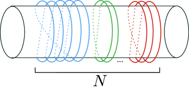
Figure 1: The black hole microstates correspond to colored partitions of $N$, which can be illustrated as a collection of multiwound colored strings: $N_{n,i}$ is the number of strings with winding number $n$ and color $i$.

An asymptotic estimate of the number of uncolored partitions was derived by Hardy and Ramanujan [72]:

$$P(N)=e^{\pi\sqrt{\frac{2N}{3}}}$$ (A.3)

to leading order in $N$. We have one color for each boson and half a color for each fermion (due to bosonization), so the total number of colors is the central charge of the seed theory,

$$N_{B}+\frac{N_{F}}{2}\equiv c_{s}.$$ (A.4)

The total number of microstates is then the number of partitions with $c_{s}$ colors:

$$P_{c_{s}}(N)=e^{2\pi\sqrt{\frac{c_{s}}{6}N}}$$ (A.5)

at large $N$. Notably, the logarithm of this quantity is the Bekenstein-Hawking entropy of the $M=0$ BTZ black hole [73] (once $\alpha^{\prime}$ corrections have been taken into account).

One can extend this reasoning to obtain (3.15). First, note that the fields $i$ are labeled by their R-symmetry charges. Focus on the four R-charged bosons, which carry

$$(J_{L},J_{R})=(\pm 1/2,\pm 1/2),\ (\pm 1/2,\mp 1/2).$$ (A.6)

In terms of the linear combinations $J_{\pm}=J_{L}\pm J_{R}$, they carry

$$(J_{+},J_{-})=(\pm 1,0),\ (0,\pm 1).$$ (A.7)

Suppose we want to estimate the number of states with fixed $J_{+}\sim O(N)$. This is a small fraction of the total number of states (A.5), since a typical colored partition will not carry much R-charge; we must fix some of the coloring so that the corresponding state carries $J_{+}$. At large $N$, the dominant contribution comes from the configurations depicted in figure 2. These configurations have $|J_{+}|$ singly-wound strings whose color corresponds to either $(J_{+},J_{-})=(1,0)$ or $(-1,0)$, depending on the sign of $J_{+}$; the remaining $N_{1}=N-|J_{+}|$ elements can be in an arbitrary configuration. The number of these configurations is the number of colored partitions of the unfixed remainder,

$$P_{c_{s}}(N_{1})=e^{2\pi\sqrt{\frac{c_{s}}{6}(N-|J_{+}|)}}$$ (A.8)

at large $N$. Configurations with some of the $J_{+}$ carried in multi-wound strings are subleading, since fewer elements will be left unfixed. Likewise subleading are configurations with $J_{+}$ carried by fermions, since the Pauli exclusion principle makes it impossible to carry all of $J_{+}$ in singly-wound fermionic strings. The collection of strings carrying $J_{+}$ can be thought of as a Bose-Einstein condensate [23].

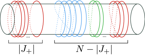
Figure 2: A typical state with positive $J_{+}\sim O(N)$ and $J_{-}\sim 0$. The red strings carry $(J_{+},J_{-})$ charges $(1,0)$ while the other strings carry other R-charges, including zero. The freedom to pick any colored partition of the remaining $N-|J_{+}|$ elements gives rise to the entropy (3.13).

To estimate the density of states at generic $J_{L/R}$ we must estimate the number of colored partitions with both $J_{+}$ and $J_{-}$ fixed. Following the same logic as above, most of these partitions will have the structure depicted in figure 3, with two condensates: one made of $|J_{+}|$ singly-wound strings carrying $(J_{+},J_{-})=(\pm 1,0)$, and another made of $|J_{-}|$ singly-wound strings carrying $(J_{+},J_{-})=(0,\pm 1)$, with the signs again determined by those of $J_{\pm}$. The entropy then comes from colored partitions of the remaining $N_{2}=N-|J_{+}|-|J_{-}|$ elements:

$$d_{J_{L},J_{R}}\approx P_{c_{s}}(N_{2})=e^{2\pi\sqrt{\frac{c_{s}}{6}(N-|J_{L}+J_{R}|-|J_{L}-J_{R}|)}}.$$ (A.9)

The theory on $M_{4}=T^{4}$ has $c_{s}=12$, which yields (3.15).

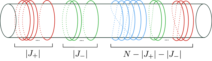
Figure 3: A typical state with positive $J_{\pm}\sim O(N)$. The red strings carry $(J_{+},J_{-})=(1,0)$ and the green strings carry $(J_{+},J_{-})=(0,1)$. The freedom to pick any colored partition of the remaining $N-|J_{+}|-|J_{-}|$ elements gives rise to the entropy (3.15).

A.2 Thermodynamic derivation of the density of states

Eq. (3.15) can be confirmed by a direct calculation of the density of states, which also enables us to study corrections. In this section we extend Appendix B of [23] to general $J_{L,R}\gtrsim O(\sqrt{N})$. Before proceeding to our extension we warm up with a review of their original calculation of $d_{J_{L},J_{R}}$, valid in the regime where $J_{L}+J_{R}\sim O(N)$ and $J_{L}-J_{R}\sim 0$. Our presentation is largely self-contained but the reader may also find it useful to consult their more detailed exposition.

Appendix B of [23] computes the density of states for $J_{+}\sim O(N)$ by starting with the partition function of the D1-D5 CFT at the orbifold point with a chemical potential $\mu_{+}$,

$$Z(\beta,\mu_{+})=\text{tr}\,e^{-\beta(N-\mu_{+}J_{+})}\,.$$ (A.10)

When $N$ is large this can be evaluated via the saddle point approximation, leading to an expression for the entropy at fixed $J_{+}$. Note that in this expression, unlike in (1.3), $\beta$ is not the inverse of the physical black hole temperature but rather an auxiliary chemical potential conjugate to the left-moving excitation number $N\equiv N_{L}$ (i.e. it is the inverse “effective temperature” $\beta_{L}$ of the left-movers); in particular, the physical Hawking temperature $T_{H}=\left(T_{L}^{-1}+T_{R}^{-1}\right)^{-1}=0$.

The seed of the orbifold has $N_{B}$ left-moving bosons and $N_{F}$ left-moving fermions. Out of these states, $n_{B}$ of the bosons have $J_{+}=1$ and another $n_{B}$ have $J_{+}=-1$. Similarly, there are $n_{F}$ fermions each with $J_{+}=\pm 1/2$. We will follow [23] in leaving the numbers of species general to faciliate comparison with their expressions. With these charge assigments, the partition function (A.10) is [23]

$$Z(\beta,\mu_{+}) =\text{tr}\ e^{-\beta(N-\mu_{+}J_{+})}$$

$$=\prod_{n=1}^{\infty}\frac{\left[(1+z^{1/2}q^{n})(1+z^{-1/2}q^{n})\right]^{n_{F}}(1+q^{n})^{N_{F}-2n_{F}}}{\left[(1-zq^{n})(1-z^{-1}q^{n})\right]^{n_{B}}(1-q^{n})^{N_{B}-2n_{B}}}$$

$$\equiv Z_{B}Z_{F}$$ (A.11)

where $q=e^{2\pi i\tau}=e^{-\beta}$ and $z=e^{2\pi i\nu}=e^{\beta\mu_{+}}$. This can be rewritten in terms of special functions as

$$Z_{B}=2^{n_{B}}q^{N_{B}/24}\eta(\tau)^{-N_{B}+3n_{B}}\left[\frac{\sin(\pi\nu)}{\theta_{1}(\pi\nu|\tau)}\right]^{n_{B}}$$ (A.12)

and

$$Z_{F}=2^{-N_{F}/2}q^{-N_{F}/24}\eta(\tau)^{-N_{F}/2}\left[\frac{\theta_{2}(\pi\nu/2|\tau)}{\cos(\pi\nu/2)}\right]^{n_{F}}\theta_{2}(0|\tau)^{N_{F}/2-n_{F}}\,.$$ (A.13)

In the thermodynamic limit $\beta\rightarrow 0$, corresponding to $N\gg 1$, the partition function simplifies:

$$Z(\beta,\mu_{+})\approx\beta^{N_{B}/2}\left(\frac{\mu_{+}}{\sin{\pi\mu_{+}}}\right)^{n_{B}}e^{\pi^{2}c_{s}/6\beta}\,.$$ (A.14)

Here $c_{s}$ is the central charge of the seed of the orbifold, $c_{s}=N_{B}+N_{F}/2$, which is $O(1)$. The first factor is the least singular as $\beta\rightarrow 0$ and can be neglected.

The saddle point approximation leads to the thermodynamic relations

$$N=-\left(\frac{\partial\log Z}{\partial\beta}\right)_{\beta\mu_{+}}=\frac{c_{s}\pi^{2}}{6\beta^{2}}+\frac{n_{B}\mu_{+}}{\beta}g(\mu_{+}),\quad\quad J_{+}=\left(\frac{\partial\log Z}{\partial(\beta\mu_{+})}\right)_{\beta}=\frac{n_{B}}{\beta}g(\mu_{+})\,,$$ (A.15)

where

$$g(x)=\frac{1}{x}-\frac{\pi}{\tan\pi x}\,.$$ (A.16)

From these expressions one obtains the entropy

$$S = \beta(N-\mu_{+}J_{+})+\log Z=\frac{c_{s}\pi^{2}}{3\beta}+n_{B}\log\left(\frac{\mu_{+}}{\sin{\pi\mu_{+}}}\right)$$ (A.17)

$$= 2\pi\sqrt{\frac{c_{s}}{6}(N-\mu_{+}J_{+})}+\log\left(\frac{\mu_{+}}{\sin{\pi\mu_{+}}}\right)$$

and the expectation value of $J_{+}$,

$$J_{+}=\frac{3\mu_{+}g(\mu_{+})^{2}}{c_{s}\pi^{2}}\left[\sqrt{1+\frac{2c_{s}N\pi^{2}}{3\mu_{+}^{2}g(\mu_{+})^{2}}}-1\right].$$ (A.18)

In the last two expressions we used $n_{B}=1$. The magnitude of $J_{+}$ is controlled by the behavior of $g(\mu_{+})$. In [23] $\mu_{+}$ is determined as follows: first, since $N-\mu_{+}J_{+}$ is not a positive operator when $|\mu_{+}|>1$, we must restrict to $|\mu_{+}|\leq 1$ in order to obtain a well-defined partition function. Next, one demands that $J_{+}\sim O(N)$. As $\mu_{+}\rightarrow 0$, $g$ vanishes linearly,

$$g(\mu_{+})=\frac{\pi^{2}}{3}\mu_{+}+O(\mu_{+}^{3}),$$ (A.19)

but it diverges as $\mu_{+}\rightarrow\pm 1$:

$$g(\mu_{+})=\frac{-1}{\mu_{+}\mp 1}\pm 1+O(\mu_{+}\mp 1).$$ (A.20)

Thus if we take $|\mu_{+}-\text{sign}(J_{+})|\sim N^{-1/2}$, (A.18) implies $J_{+}\sim O(N)$ and we have the desired enhancement. Making this choice in (A.17), the density of states in this regime is

$$d_{J_{+},J_{-}}=e^{2\pi\sqrt{\frac{c_{s}}{6}(N-|J_{+}|)}}\quad\quad\text{when }\quad\quad J_{+}\sim O(N),\ J_{-}\sim 0$$ (A.21)

up to subleading corrections in $N$. This completes our review of [23].

To study the density of states at general $J_{L/R}$ we must also turn on a chemical potential for $J_{-}$:

$$Z(\beta,\mu_{+},\mu_{-}) =\text{tr}\ e^{-\beta(N-\mu_{+}J_{+}-\mu_{-}J_{-})}$$

$$=\prod_{n=1}^{\infty}\frac{\left[(1+z^{1/2}q^{n})(1+z^{-1/2}q^{n})(1+\tilde{z}^{1/2}q^{n})(1+\tilde{z}^{-1/2}q^{n})\right]^{n_{F}}(1+q^{n})^{N_{F}-4n_{F}}}{\left[(1-zq^{n})(1-z^{-1}q^{n})(1-{\tilde{z}}q^{n})(1-{\tilde{z}}^{-1}q^{n})\right]^{n_{B}}(1-q^{n})^{N_{B}-4n_{B}}}$$

$$\equiv Z_{B}Z_{F},$$ (A.22)

where $q=e^{2\pi i\tau}=e^{-\beta}$, $z=e^{2\pi i\nu}=e^{\beta\mu_{+}}$ and $\tilde{z}=e^{2\pi i\tilde{\nu}}=e^{\beta\mu_{-}}$. The second line follows from the fact that the theory has $n_{B}$ states with charges $(J_{+},J_{-})=(\pm 1,0),(0,\pm 1)$, and similarly for the fermions. We find

$$Z_{B} =2^{2n_{B}}q^{N_{B}/24}\eta(\tau)^{-N_{B}+6n_{B}}\left[\frac{\sin(\pi\nu_{+})}{\theta_{1}(\pi\nu_{+}|\tau)}\right]^{n_{B}}\left[\frac{\sin(\pi\nu_{-})}{\theta_{1}(\pi\nu_{-}|\tau)}\right]^{n_{B}}$$ (A.23)

and

$$Z_{F} =2^{-N_{F}/2}q^{-N_{F}/24}\eta(\tau)^{-N_{F}/2}\left[\frac{\theta_{2}(\pi\nu_{+}/2|\tau)}{\cos(\pi\nu_{+}/2)}\right]^{n_{F}}\left[\frac{\theta_{2}(\pi\nu_{-}/2|\tau)}{\cos(\pi\nu_{-}/2)}\right]^{n_{F}}\theta_{2}(0|\tau)^{N_{F}/2-2n_{F}}.$$ (A.24)

In the thermodynamic limit $\beta\rightarrow 0$ corresponding to large $N$, the partition function once again simplifies:

$$Z(\beta,\mu_{+},\mu_{-})\approx\beta^{N_{B}/2}\left(\frac{\mu_{+}}{\sin{\pi\mu_{-}}}\right)^{n_{B}}\left(\frac{\mu_{+}}{\sin{\pi\mu_{-}}}\right)^{n_{B}}e^{\pi^{2}c_{s}/6\beta}.$$ (A.25)

The saddle point analysis leads to

$$N =-\left(\frac{\partial\log Z}{\partial\beta}\right)_{\beta\mu_{+},\beta\mu_{-}}=\frac{c_{s}\pi^{2}}{6\beta^{2}}+\frac{n_{B}\mu_{+}}{\beta}g(\mu_{+})+\frac{n_{B}\mu_{-}}{\beta}g(\mu_{-}),$$

$$J_{+} =\left(\frac{\partial\log Z}{\partial(\beta\mu_{+})}\right)_{\beta,\beta\mu_{-}}=\frac{n_{B}}{\beta}g(\mu_{+}),\quad\quad J_{-}=\left(\frac{\partial\log Z}{\partial(\beta\mu_{-})}\right)_{\beta,\beta\mu_{+}}=\frac{n_{B}}{\beta}g(\mu_{-}),$$ (A.26)

and the entropy

$$S =\beta(N-\mu_{+}J_{+}-\mu_{-}J_{-})+\log Z=\frac{c_{s}\pi^{2}}{3\beta}+n_{B}\log\left(\frac{\mu_{+}}{\sin{\pi\mu_{+}}}\right)+n_{B}\log\left(\frac{\mu_{-}}{\sin{\pi\mu_{-}}}\right)$$

$$=2\pi\sqrt{\frac{c_{s}}{6}(N-\mu_{+}J_{+}-\mu_{-}J_{-})}+\log\left(\frac{\mu_{+}}{\sin{\pi\mu_{+}}}\right)+\log\left(\frac{\mu_{-}}{\sin{\pi\mu_{-}}}\right)$$ (A.27)

where we again used $n_{B}=1$. Similarly, one finds the R-charges

$$J_{\pm}=\frac{3f_{\pm}}{c_{s}\pi^{2}}\left[\sqrt{1+\frac{2c_{s}N\pi^{2}g(\mu_{\pm})^{2}}{3f_{\pm}^{2}}}-1\right]$$ (A.28)

where

$$f_{\pm}=g(\mu_{\pm})\left[\mu_{\pm}\ g(\mu_{\pm})+\mu_{\mp}\ g(\mu_{\mp})\right].$$ (A.29)

As above we determine $\mu_{\pm}$ in the density of states at $J_{\pm}\sim O(N)$ by requiring that (A.28) implies $J_{\pm}\sim O(N)$. Once again this implies $|\mu_{\pm}-{\rm sign}(J_{\pm})|\sim N^{-1/2}$ and so

$$d_{J_{L},J_{R}}=e^{2\pi\sqrt{\frac{c_{s}}{6}(N-|J_{+}|-|J_{-}|)}}\quad\quad\text{when }\quad\quad(J_{+},J_{-})\sim O({N}).$$ (A.30)

This is the expression we used to evaluate $\chi$ in (3.16).

So far we have computed the density of states when $J_{L/R}\sim O(N)$. However, typical microstates of the $M=0$ BTZ black hole have $J_{L/R}\sim O(\sqrt{N})$. When $J_{L/R}\sim O(\sqrt{N})$, we find that the density of states is

$$d_{J_{L},J_{R}}=e^{2\pi\sqrt{\frac{c_{s}}{6}\left[N-\gamma_{+}(J_{+})|J_{+}|-\gamma_{-}(J_{-})|J_{-}|\right]}}\quad\quad\text{when }\quad\quad(J_{+},J_{-})\sim O(\sqrt{N}).$$ (A.31)

We have used time-reversal invariance to fix $\mu_{\pm}=\gamma_{\pm}\ \text{sign}(J_{\pm})$ for some $0<\gamma_{\pm}<1$, but the $\gamma_{\pm}(J_{\pm})$ must be determined numerically by inverting the transcendental relation (A.28). We will now quantify the error in our computation of $\chi$ in (3.16) caused by our use of (A.30) over the whole range of $J_{L/R}$.

We should have used (A.31) instead of (A.30) in the appropriate region of the integral in (3.16) when we computed $\chi$. Consider the fractional error we made in computing $\chi$,

$$\frac{\Delta\chi}{\chi}=\frac{\int_{-N}^{N}dJ_{+}\ dJ_{-}\ \left[e^{2\pi\sqrt{\frac{c_{s}}{6}\left[N-\gamma_{+}(J_{+})|J_{+}|-\gamma_{-}(J_{-})|J_{-}|\right]}}-e^{2\pi\sqrt{\frac{c_{s}}{6}\left(N-|J_{+}|-|J_{-}|\right)}}\right]\left(J_{L}^{2}+J_{R}^{2}\right)}{\int_{-N}^{N}dJ_{+}\ dJ_{-}\ e^{2\pi\sqrt{\frac{c_{s}}{6}\left(N-|J_{+}|-|J_{-}|\right)}}\left(J_{L}^{2}+J_{R}^{2}\right)}.$$ (A.32)

To be complete we have integrated over the entire range of $J_{\pm}$, though the contribution from $J_{\pm}\sim O(N)$ vanishes since (A.30) approaches (A.31) in that regime. Our conclusion in the main text that $\alpha\sim O(c^{0})$ will hold true so long as the fractional error does not scale with $N$.

We will analyze the simpler quantity

$$\varepsilon(m)\equiv\frac{\int_{0}^{m\sqrt{N}}dJ_{+}\ \left[e^{\sqrt{N-\gamma_{+}(J_{+})|J_{+}|}}-e^{\sqrt{N-|J_{+}|}}\right]\ J_{+}^{2}}{\int_{0}^{N}dJ_{+}\ e^{\sqrt{N-|J_{+}|}}\ J_{+}^{2}}.$$ (A.33)

This quantity misses contributions from $|J_{+}|~{}>~{}m\sqrt{N}$ but such contributions will be negligible when $m$ is sufficiently large. Here $\gamma_{+}\equiv\mu_{+}\ \text{sign}(J_{+})$, obtained by inverting (A.18), is plotted in the left panel of figure 4. In the large-$N$ limit and for sufficiently large $m$, $\varepsilon$ is equal to the fractional error (A.32) up to an overall $O(1)$ multiplicative factor (see the remarks in footnote 8).

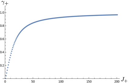
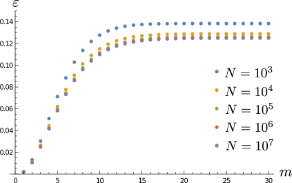
Figure 4: Left: $\gamma_{+}(J_{+})$ for $N=1000$.          Right: $\varepsilon(m)$ at large $N$.

In the right panel of figure 4 we plot $\varepsilon(m)$ numerically for several different values of $N$. There are two salient features. The first is the rapid convergence in $m$ to an asymptotic value $\varepsilon_{\star}$: we do not need to take $m$ very large in order to obtain a good approximation of $\Delta\chi/\chi$, once the $O(1)$ multiplicative factor is restored. This follows from the fact that $\gamma_{+}$ is monotonic and approaches 1 quite rapidly above $J_{+}\sim O(\sqrt{N})$. The second feature is the crucial one: convergence $\varepsilon_{\star}\rightarrow 0.1249$ at large $N$. This leads to our conclusion that $\alpha\sim O(c^{0})$.

References

- [1] X. Dong, D. Harlow and A. C. Wall, Reconstruction of Bulk Operators within the Entanglement Wedge in Gauge-Gravity Duality, Phys. Rev. Lett. 117 (2016), no. 2, 021601, 1601.05416
- [2] T. Faulkner, R. G. Leigh, O. Parrikar and H. Wang, Modular Hamiltonians for Deformed Half-Spaces and the Averaged Null Energy Condition, JHEP 09 (2016) 038, 1605.08072
- [3] A. C. Wall, A Proof of the generalized second law for rapidly-evolving Rindler horizons, Phys. Rev. D82 (2010) 124019, 1007.1493
- [4] N. Lashkari, M. B. McDermott and M. Van Raamsdonk, Gravitational dynamics from entanglement ’thermodynamics’, JHEP 04 (2014) 195, 1308.3716
- [5] D. D. Blanco, H. Casini, L.-Y. Hung and R. C. Myers, Relative Entropy and Holography, JHEP 08 (2013) 060, 1305.3182
- [6] T. Faulkner, M. Guica, T. Hartman, R. C. Myers and M. Van Raamsdonk, Gravitation from Entanglement in Holographic CFTs, JHEP 03 (2014) 051, 1312.7856
- [7] E. Hijano and P. Kraus, A new spin on entanglement entropy, JHEP 12 (2014) 041, 1406.1804
- [8] T. Faulkner, F. M. Haehl, E. Hijano, O. Parrikar, C. Rabideau and M. Van Raamsdonk, Nonlinear Gravity from Entanglement in Conformal Field Theories, JHEP 08 (2017) 057, 1705.03026
- [9] F. M. Haehl, E. Hijano, O. Parrikar and C. Rabideau, Higher Curvature Gravity from Entanglement in Conformal Field Theories, 1712.06620
- [10] N. Lashkari, Modular Hamiltonian for Excited States in Conformal Field Theory, Phys. Rev. Lett. 117 (2016), no. 4, 041601, 1508.03506
- [11] G. Sárosi and T. Ugajin, Relative entropy of excited states in two dimensional conformal field theories, JHEP 07 (2016) 114, 1603.03057
- [12] N. Bao and H. Ooguri, Distinguishability of black hole microstates, Phys. Rev. D96 (2017), no. 6, 066017, 1705.07943
- [13] S. Ryu and T. Takayanagi, Holographic derivation of entanglement entropy from AdS/CFT, Phys. Rev. Lett. 96 (2006) 181602, hep-th/0603001
- [14] V. E. Hubeny, M. Rangamani and T. Takayanagi, A Covariant holographic entanglement entropy proposal, JHEP 07 (2007) 062, 0705.0016
- [15] A. L. Fitzpatrick, J. Kaplan and M. T. Walters, Universality of Long-Distance AdS Physics from the CFT Bootstrap, JHEP 08 (2014) 145, 1403.6829
- [16] C. T. Asplund, A. Bernamonti, F. Galli and T. Hartman, Holographic Entanglement Entropy from 2d CFT: Heavy States and Local Quenches, JHEP 02 (2015) 171, 1410.1392
- [17] E. Perlmutter, Virasoro conformal blocks in closed form, JHEP 08 (2015) 088, 1502.07742
- [18] M. Banados, C. Teitelboim and J. Zanelli, The Black hole in three-dimensional space-time, Phys. Rev. Lett. 69 (1992) 1849–1851, hep-th/9204099
- [19] M. Banados, M. Henneaux, C. Teitelboim and J. Zanelli, Geometry of the (2+1) black hole, Phys. Rev. D48 (1993) 1506–1525, gr-qc/9302012, [Erratum: Phys. Rev.D88,069902(2013)]
- [20] A. Strominger and C. Vafa, Microscopic origin of the Bekenstein-Hawking entropy, Phys. Lett. B379 (1996) 99–104, hep-th/9601029
- [21] P. Calabrese, J. Cardy and E. Tonni, Entanglement entropy of two disjoint intervals in conformal field theory II, J. Stat. Mech. 1101 (2011) P01021, 1011.5482
- [22] S. Giusto and R. Russo, Entanglement Entropy and D1-D5 geometries, Phys. Rev. D90 (2014), no. 6, 066004, 1405.6185
- [23] V. Balasubramanian, P. Kraus and M. Shigemori, Massless black holes and black rings as effective geometries of the D1-D5 system, Class. Quant. Grav. 22 (2005) 4803–4838, hep-th/0508110
- [24] P. Calabrese and J. Cardy, Entanglement entropy and conformal field theory, J. Phys. A42 (2009) 504005, 0905.4013
- [25] T. Hartman, Entanglement Entropy at Large Central Charge, 1303.6955
- [26] O. Lunin and S. D. Mathur, AdS / CFT duality and the black hole information paradox, Nucl. Phys. B623 (2002) 342–394, hep-th/0109154
- [27] S. D. Mathur, The Fuzzball proposal for black holes: An Elementary review, Fortsch. Phys. 53 (2005) 793–827, hep-th/0502050
- [28] I. Bena and N. P. Warner, Black holes, black rings and their microstates, Lect. Notes Phys. 755 (2008) 1–92, hep-th/0701216
- [29] S. D. Mathur, Fuzzballs and the information paradox: A Summary and conjectures, 0810.4525
- [30] V. Balasubramanian, J. de Boer, S. El-Showk and I. Messamah, Black Holes as Effective Geometries, Class. Quant. Grav. 25 (2008) 214004, 0811.0263
- [31] I. Bena and N. P. Warner, Resolving the Structure of Black Holes: Philosophizing with a Hammer, 1311.4538
- [32] F. Chen, B. Michel, J. Polchinski and A. Puhm, Journey to the Center of the Fuzzball, JHEP 02 (2015) 081, 1408.4798
- [33] F. C. Eperon, H. S. Reall and J. E. Santos, Instability of supersymmetric microstate geometries, 1607.06828
- [34] D. Marolf, B. Michel and A. Puhm, A rough end for smooth microstate geometries, JHEP 05 (2017) 021, 1612.05235
- [35] E. J. Martinec and S. Massai, String Theory of Supertubes, 1705.10844
- [36] W. Lerche, C. Vafa and N. P. Warner, Chiral Rings in N=2 Superconformal Theories, Nucl. Phys. B324 (1989) 427–474
- [37] O. Lunin and S. D. Mathur, Three-point functions for M(N)/S(N) orbifolds with N = 4 supersymmetry, Commun. Math. Phys. 227 (2002) 385–419, hep-th/0103169
- [38] J. R. David, G. Mandal and S. R. Wadia, Microscopic formulation of black holes in string theory, Phys. Rept. 369 (2002) 549–686, hep-th/0203048
- [39] I. Kanitscheider, K. Skenderis and M. Taylor, Fuzzballs with internal excitations, JHEP 0706 (2007) 056, 0704.0690
- [40] R. Dijkgraaf, Instanton strings and hyperKahler geometry, Nucl. Phys. B543 (1999) 545–571, hep-th/9810210
- [41] J. M. Maldacena, The Large N limit of superconformal field theories and supergravity, Int. J. Theor. Phys. 38 (1999) 1113–1133, hep-th/9711200, [Adv. Theor. Math. Phys.2,231(1998)]
- [42] A. Strominger, Black hole entropy from near horizon microstates, JHEP 02 (1998) 009, hep-th/9712251
- [43] O. Lunin, J. M. Maldacena and L. Maoz, Gravity solutions for the D1-D5 system with angular momentum, hep-th/0212210
- [44] O. Lunin and S. D. Mathur, Metric of the multiply wound rotating string, Nucl. Phys. B610 (2001) 49–76, hep-th/0105136
- [45] M. Baggio, J. de Boer and K. Papadodimas, A non-renormalization theorem for chiral primary 3-point functions, JHEP 07 (2012) 137, 1203.1036
- [46] S. Giusto, E. Moscato and R. Russo, AdS3 holography for 1/4 and 1/8 BPS geometries, JHEP 11 (2015) 004, 1507.00945
- [47] I. Bena, M. Shigemori and N. P. Warner, Black-Hole Entropy from Supergravity Superstrata States, JHEP 10 (2014) 140, 1406.4506
- [48] E. J. Martinec and B. E. Niehoff, Hair-brane Ideas on the Horizon, JHEP 11 (2015) 195, 1509.00044
- [49] I. Bena, S. Giusto, R. Russo, M. Shigemori and N. P. Warner, Habemus Superstratum! A constructive proof of the existence of superstrata, JHEP 05 (2015) 110, 1503.01463
- [50] I. Bena, S. Giusto, E. J. Martinec, R. Russo, M. Shigemori, D. Turton and N. P. Warner, Smooth horizonless geometries deep inside the black-hole regime, Phys. Rev. Lett. 117 (2016), no. 20, 201601, 1607.03908
- [51] I. Bena, E. Martinec, D. Turton and N. P. Warner, M-theory Superstrata and the MSW String, JHEP 06 (2017) 137, 1703.10171
- [52] I. Bena, D. Turton, R. Walker and N. P. Warner, Integrability and Black-Hole Microstate Geometries, JHEP 11 (2017) 021, 1709.01107
- [53] A. Tyukov, R. Walker and N. P. Warner, Tidal Stresses and Energy Gaps in Microstate Geometries, 1710.09006
- [54] I. Bena, S. Giusto, E. J. Martinec, R. Russo, M. Shigemori, D. Turton and N. P. Warner, Asymptotically-flat supergravity solutions deep inside the black-hole regime, 1711.10474
- [55] V. Jejjala, O. Madden, S. F. Ross and G. Titchener, Non-supersymmetric smooth geometries and D1-D5-P bound states, Phys. Rev. D71 (2005) 124030, hep-th/0504181
- [56] I. Bena, A. Puhm and B. Vercnocke, Metastable Supertubes and non-extremal Black Hole Microstates, JHEP 04 (2012) 100, 1109.5180
- [57] I. Bena, A. Puhm and B. Vercnocke, Non-extremal Black Hole Microstates: Fuzzballs of Fire or Fuzzballs of Fuzz ?, JHEP 1212 (2012) 014, 1208.3468
- [58] I. Bena, G. Bossard, S. Katmadas and D. Turton, Bolting Multicenter Solutions, JHEP 01 (2017) 127, 1611.03500
- [59] G. Bossard, S. Katmadas and D. Turton, Two Kissing Bolts, 1711.04784
- [60] H. Lin, O. Lunin and J. M. Maldacena, Bubbling AdS space and 1/2 BPS geometries, JHEP 0410 (2004) 025, hep-th/0409174
- [61] R. C. Myers and O. Tafjord, Superstars and giant gravitons, JHEP 11 (2001) 009, hep-th/0109127
- [62] V. Balasubramanian, V. Jejjala and J. Simon, The Library of Babel, Int. J. Mod. Phys. D14 (2005) 2181–2186, hep-th/0505123
- [63] V. Balasubramanian, J. de Boer, V. Jejjala and J. Simon, The Library of Babel: On the origin of gravitational thermodynamics, JHEP 12 (2005) 006, hep-th/0508023
- [64] C. Kim, K. K. Kim and O.-K. Kwon, Holographic Entanglement Entropy of Anisotropic Minimal Surfaces in LLM Geometries, Phys. Lett. B759 (2016) 395–401, 1605.00849
- [65] A. L. Fitzpatrick and J. Kaplan, Conformal Blocks Beyond the Semi-Classical Limit, JHEP 05 (2016) 075, 1512.03052
- [66] A. L. Fitzpatrick and J. Kaplan, A Quantum Correction To Chaos, JHEP 05 (2016) 070, 1601.06164
- [67] A. L. Fitzpatrick, J. Kaplan, D. Li and J. Wang, On information loss in AdS3/CFT2, JHEP 05 (2016) 109, 1603.08925
- [68] A. L. Fitzpatrick, J. Kaplan, D. Li and J. Wang, Exact Virasoro Blocks from Wilson Lines and Background-Independent Operators, JHEP 07 (2017) 092, 1612.06385
- [69] N. Anand, H. Chen, A. L. Fitzpatrick, J. Kaplan and D. Li, An Exact Operator That Knows Its Location, 1708.04246
- [70] H. Chen, A. L. Fitzpatrick, J. Kaplan and D. Li, The AdS3 Propagator and the Fate of Locality, 1712.02351
- [71] T. Faulkner and H. Wang, Probing beyond ETH at large , 1712.03464
- [72] G. H. Hardy and S. Ramanujan, Asymptotic Formulae in Combinatory Analysis, Proceedings of the London Mathematical Society s2-17 (1918), no. 1, 75–115
- [73] A. Dabholkar, Exact counting of black hole microstates, Phys. Rev. Lett. 94 (2005) 241301, hep-th/0409148