On the consistency of adaptive multiple tests

Abstract

Much effort has been done to control the ”false discovery rate” (FDR) when $m$ hypotheses are tested simultaneously. The FDR is the expectation of the ”false discovery proportion” $\text{FDP}=V/R$ given by the ratio of the number of false rejections $V$ and all rejections $R$. In this paper, we have a closer look at the FDP for adaptive linear step-up multiple tests. These tests extend the well known Benjamini and Hochberg test by estimating the unknown amount $m_{0}$ of the true null hypotheses. We give exact finite sample formulas for higher moments of the FDP and, in particular, for its variance. Using these allows us a precise discussion about the consistency of adaptive step-up tests. We present sufficient and necessary conditions for consistency on the estimators $\widehat{m}_{0}$ and the underlying probability regime. We apply our results to convex combinations of generalized Storey type estimators with various tuning parameters and (possibly) data-driven weights. The corresponding step-up tests allow a flexible adaptation. Moreover, these tests control the FDR at finite sample size. We compare these tests to the classical Benjamini and Hochberg test and discuss the advantages of it.

and

1 Introduction

Testing $m\geq 2$ hypotheses simultaneously is a frequent issue in statistical practice, e.g. in genomic research. A widely used criterion for deciding which of these hypotheses should be rejected is the so-called ”false discovery rate” (FDR) promoted by Benjamini and Hochberg [3]. The FDR is the expectation of the ”false discovery proportion” (FDP), the ratio $\text{FDP}=V/R$ of the number of false rejections $V$ and all rejections $R$. Let a level $\alpha\in(0,1)$ be given. Under the so-called basic independence (BI) assumption we have FDR$=(m_{0}/m)\alpha$ for the classical Benjamini and Hochberg linear step-up test, briefly denoted by BH test. Here, $m_{0}$ is the unknown amount of true null hypotheses. To achieve a higher power it is of great interest to exhaust the FDR as good as possible. Especially, if $m_{0}/m=c$ is not close to $1$ there is space for improvement of the BH test. That is why since the beginning of this century the interest of adaptive tests grows. The idea is to estimate $m_{0}$ by an appropriate estimator $\widehat{m}_{0}$ in a first step and to apply the BH test for the (data depended) level $\alpha^{\prime}=(m/\widehat{m}_{0})\alpha$ in the second step. Heuristically, we obtain for a good estimator $\widehat{m}_{0}\approx m_{0}$ that FDR$\;\approx\alpha$. Benjamini and Hochberg [4] suggested an early estimator for $m_{0}$ leading to an FDR controlling test. Before them Schweder and Spjøtvoll [31] already discussed estimators for $m_{0}$ using plots of the empirical distribution function of the $p$-values. The number of estimators suggested in the literature is huge, here only a short selection: Benjamini et al. [5], Blanchard and Roquain [7, 8] and Zeisel et al. [36]. We want to emphasize the papers of the Storey [33] and Storey et al. [34] and, in particular, the Storey estimator based on a tuning parameter $\lambda$. We refer to Storey and Tibshirani [35] for a discussion of the adjustment of the tuning parameter $\lambda$. Generalized Storey estimators with data dependent weights, which were already discussed by Heesen and Janssen [21], will be our prime example for our general results. A nice property of them is that we have finite sample FDR control, see [21]. Sufficient conditions for finite sample FDR control on general estimators $\widehat{m}_{0}$ can be found in Sarkar [28] and Heesen and Janssen [20, 21].
Beside the FDR control there are also other control criteria, for example the family-wise error rate FWER$=P(V>0)$. Also for the control of FWER adaptive tests, i.e. tests using an (plug-in) estimator for $m_{0}$, are used and discussed in the literature, see e.g. Finner and Gontscharuk [14] and Sarkar et al. [29].
Stochastic process methods were applied to study the asymptotic behavior of the FDP, among others to calculate asymptotic confidence intervals, and the familywise error rate (FWER) in detail, see Genovese and Wassermann [17], Meinshausen and Bühlmann [24], Meinshausen and Rice [25] and Neuvial [26]. Dealing with a huge amount of $p$-values the fluctuation of the FDP becomes, of course, relevant. Ferreira and Zwinderman [12] presented formulas for higher moments of FDP for the BH test and Roquain and Villers [27] did so for step-up and step-down tests with general (but data independent) critical values. We generalize these formulas to adaptive step-up tests using general estimators $\widehat{m}_{0}$ for $m_{0}$. In particular, we derive an exact finite sample formula for the variability of FDP. As an application of this we discuss the consistency of FDP and present sufficient and necessary conditions for it. We also discuss the more challenging case of sparsity in the sense that $m_{0}/m\to 1$ as $m\to\infty$. This situation can be compared to the one of Abramovich et al. [1], who derived an estimator of the (sparse) mean of a multivariate normal distribution using FDR procedures.

Outline of the results. In Section 2 we introduce the model as well as the adaptive step-up tests, and in particular the generalized Storey estimators which serve as prime examples. Section 3 provides exact finite sample variance formulas for the FDP under the BI model. Extensions to higher moments can be found in the appendix, see Section 9. These results apply to the variability and the consistency of FDP, see Section Section 4. Roughly speaking we have consistency if we have stable estimators $\widehat{m}_{0}/m\approx C_{0}$ and the number of rejections tends to infinity. Section 5 is devoted to concrete adaptive step-up tests mainly based on the convex combinations of generalized Storey estimators with data dependent weights. We will see that consistency cannot be achieved in general. Under mild assumptions the adaptive tests based on the estimators mentioned above are superior compared to the BH test: The FDR is more exhausted but remains finitely controlled by the level $\alpha$. Furthermore, they are consistent at least when the BH test is consistent. In Section 6 we discuss least favorable configurations which serve as useful technical tools. For the reader’s convenience we add a discussion and summary of the paper in Section 7. All proofs are collected in Section 8.

2 Preliminaries

2.1 The model and general step-up tests

Let us first describe the model and the procedures. A multiple testing problem consists on $m$ null hypotheses $(H_{i,m},p_{i,m})$ with associated $p$-value $0\leq p_{i,m}\leq 1$ on a common probability space $(\Omega_{m},\mathcal{A}_{m},P_{m})$. We will always use the basic independence (BI) assumption given by

1. The set of hypotheses can be divided in the disjoint union $I_{0,m}\bigcup I_{1,m}=\{1,...,m\}$ of unknown portions of true null $I_{0,m}$ and false null $I_{1,m}$, respectively. Denote by $m_{j}=\#I_{j,m}$ the cardinality of $I_{j,m}$ for $j=0,1$.

2. The vectors of $p$-values $\left(p_{i,m}\right)_{i\in I_{0,m}}$ and $\left(p_{i,m}\right)_{i\in I_{1,m}}$ are independent, where each dependence structure is allowed for the $p$-values $\left(p_{i,m}\right)_{i\in I_{1}}$ for the false hypotheses.

3. The $p$-values $\left(p_{i,m}\right)_{i\in I_{0,m}}$ of the true null are independent and uniformly distributed on $[0,1]$, i.e. $P_{m}(p_{i,m}\leq x)=x$ for all $x\in[0,1]$.

Throughout the paper let $m_{0}\geq 1$ be nonrandom. As in Heesen and Janssen [21] the results can be extended to more general models with random $m_{0}$ by conditioning under $m_{0}$. By using this modification the results easily carry over to familiar mixture models discussed, for instance, by Abramovich et al. [1] and Genovese and Wassermann [17]. We study adaptive multiple step-up tests with estimated critical values extending the famous Benjamini and Hochberg [3] step-up test, briefly denoted by BH test. In the following we recall the definition of this kind of tests. Let

(2.1) $$0=\alpha_{0:m}<\alpha_{1:m}\leq\alpha_{2:m}\leq\ldots\leq\alpha_{m:m}<1$$

denote possibly data dependent critical values. As an example for the critical values we recall the ones for the BH test, which do not depend on the data:

$$\alpha_{i:m}^{\text{BH}}=\frac{i}{m}\alpha.$$

If $p_{1:m}\leq p_{2:m}\leq\ldots\leq p_{m:m}$ denote the ordered $p$-value then the number of rejections is given by

$$R_{m}:=\max\{i=0,\ldots,m:p_{i:m}\leq\alpha_{i:m}\},\text{ where }p_{0:m}:=0,$$

and the multiple procedure acts as follows:

$$\text{reject }H_{i,m}\text{ iff }p_{i,m}\leq\alpha_{R_{m}:m}.$$

Moreover, let

(2.2) $$V_{m}:=\#\{i\in I_{0,m}\cup\{0\}:p_{i:m}\leq\alpha_{i:m}\}$$

be the number of falsely rejected null hypothesis. Then the false discovery rate $\text{FDR}_{m}$ and the false discovery proportion $\text{FDP}_{m}$ are given by

(2.3) $$\text{FDP}_{m}=\frac{V_{m}}{R_{m}}\text{ and }\text{FDR}_{m}={\mathbb{E}}\Bigl{(}\frac{V_{m}}{R_{m}}\Bigr{)}\text{ with }\frac{0}{0}=0.$$

Good multiple tests like the BH test or the frequently applied adaptive test of Storey et al. [34] control the FDR at a pre-specified acceptance error bound $\alpha$ at least under the BI assumption. Besides the control, two further aspects are of importance and discussed below:

1. To make the test sensitive for signal detection the FDR should exhaust the level $\alpha$ as best as possible.

2. On the other hand the variability of the FDP, see (2.3), is of interest in order to judge the stability of the test.

For a large class of adaptive tests exact FDR formulas were established in Heesen and Janssen [21]. Here the reader can find new $\alpha$-controlling tests with high FDR. These formulas are now completed by formulas for exact higher FDP moments and, in particular, for the variance. These results open the door for a discussion about the consistency of multiple tests, i.e.

(2.4) $$\frac{V_{m}}{R_{m}}-{\mathbb{E}}\Bigl{(}\frac{V_{m}}{R_{m}}\Bigr{)}\xrightarrow{P_{m}}0\text{ or equivalently }\text{Var}\Bigl{(}\frac{V_{m}}{R_{m}}\Bigr{)}\to 0.$$

Specific results are discussed in Sections 4 and 5. If $\liminf_{m\to\infty}\text{FDR}_{m}>0$ then we have the following necessary condition for consistency:

(2.5) $$\lim_{m\to\infty}P_{m}(V_{m}>0)=1.$$

As already stated we can not expect consistency in general. In the following we discuss the BH test for two extreme case.

Example 2.1.

1. Let $m_{1}\geq 0$ be fixed. Then $P_{m}(V_{m}^{\text{BH}}=0)$ is minimal for the so-called Dirac uniform configuration DU$(m,m_{1})$, where all entries of $(p_{i,m})_{i\in I_{1,m}}$ are equal to zero. Under this configuration $V_{m}^{\text{BH}}(\alpha,m_{1})\to V_{\text{SU}}(\alpha,m_{1})$ in distribution with

   $$P\Bigl{(}V_{\text{SU}}(\alpha,m_{1})=0\Bigr{)}=(1-\alpha)\exp(-m_{1}\alpha),$$

   see Finner and Roters [16] and Theorem 4.8 of Scheer [30]. The limit variable belongs to the class of linear Poisson distributions, see Finner et al. [15], Jain [22] and Consul and Famoye [10]. Hence, the BH-test is never consistent under BI for fixed $m_{1}$ since (2.5) is violated.

2. Another extreme case is given by i.i.d. distributed $p$-value $(p_{i,m})_{i\in I_{m,1}}$. Suppose that $p_{i,m}$, $i\in I_{1,m}$, is uniformly distributed on $[0,\lambda]$, where $\alpha<\lambda<1$. Then the BH-tests are not consistent, see Theorem 5.1(b).

More information about DU$(m,m_{1})$ and least favorable configurations can be found in Section 6. The requirement for consistency will be somehow in between these two extreme cases where the assumption $m_{1}\to\infty$ will be always needed.

2.2 Our step-up tests and underlying assumptions

In the following we introduce the adaptive step-up tests we consider in this paper. Let $0<\alpha<1$ be a fixed level and let $\lambda$, $\alpha\leq\lambda<1$, be a tuning parameter and we agree that no null ${\mathcal{H}}_{i,m}$ with $p_{i,m}>\lambda$ should be rejected. The latter is not restrictive for practice since it is very unusual to reject a null if the corresponding $p$-value exceeds, for instance, $1/2$. We divide the range $[0,1]$ of the $p$-values in a decision region $[0,\lambda]$, where all ${\mathcal{H}}_{i,m}$ with $p_{i,m}\leq\lambda$ have a chance to be rejected, and an estimation region $(\lambda,1]$, where $p_{i,m}>\lambda$ are used to estimate $m_{0}$, see Figure 1.

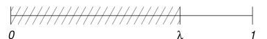
Figure 1: Decision region $[0,\lambda]$ (dashed) and estimation region $(\lambda,1]$.

To be more specific we consider estimators $\widehat{m}_{0}$ of the form

(2.6) $$\widehat{m}_{0}=\widehat{m}_{0}((\widehat{F}_{m}(t))_{t\geq\lambda})>0$$

for estimating $m_{0}$, which are measurable functions depending only on $(\widehat{F}_{m}(t))_{t\geq\lambda}$. As usual we denote by $\widehat{F}_{m}$ the empirical distribution function of the $p$-values $p_{1,m},\ldots,p_{m,m}$. As motivated in the introduction we now plug-in these estimators in the BH test. Doing this we obtain the data driven critical values

(2.7) $$\widehat{\alpha}_{i:m}=\min\Bigl{\{}\left(\frac{i}{\widehat{m}_{0}}\alpha\right),\lambda\Bigr{\}},\quad i=1,\ldots,n,$$

where we promote to use the upper bound $\lambda$ as Heesen and Janssen [21] already did. The following two quantities will be rapidly used: Through

(2.8) $$R_{m}(t)=m\widehat{F}_{m}(t)\quad\mbox{and}\quad V_{m}(t)=\sum_{i\in I_{0}}1\{p_{i,m}\leq t\},\;t\in[0,1].$$

Throughout this paper, we investigate different mild assumptions. For our main results we fix the following two:

1. Suppose that

   $$\frac{m_{0}}{m}\to\kappa_{0}\in(0,1].$$

2. Suppose that $\widehat{m}_{0}$ is always positive and

   $$\frac{\lambda}{\alpha}\widehat{m}_{0}\geq R_{m}(\lambda).$$

If only $0<\liminf_{m\to\infty}m_{0}/m$ is valid then our results apply to appropriate subsequences. The most interesting case is $\kappa_{0}>\alpha$ since otherwise (if $m_{0}/m\leq\alpha$) the FDR can be controlled, i.e. $\text{FDR}_{m}\leq\alpha$, by rejecting everything.

Remark 2.2.

1. Under (A2) the FDR of the adaptive multiple test was obtained for the BI model by Heesen and Janssen [21]:

   (2.9) $$\text{FDR}_{m}=\frac{\alpha}{\lambda}{\mathbb{E}}\Bigl{(}\frac{V_{m}(\lambda)}{\widehat{m}_{0}}\Bigr{)}.$$

   In particular, we obtain

   $$\text{FDR}_{m}\leq{\mathbb{E}}\Bigl{(}\frac{V_{m}(\lambda)}{R_{m}(\lambda)}\Bigr{)}\leq P_{m}(V_{m}(\lambda)>0),$$

   where the upper bound is always strictly smaller than $1$ for finite $m$.

2. If (A2) is not fulfilled then consider the estimator $\max\{\widehat{m}_{0},(\alpha/\lambda)R_{m}(\lambda)\}$ instead of $\widehat{m}_{0}$. Note that both estimators lead to the same critical values $\alpha_{i:m}$ and so the assumption (A2) is not restrictive.

A prominent example for an adaptive test controlling the FDR by $\alpha$ is given by the Storey estimator (2.11):

(2.10) $${\widehat{m}}_{0}^{\text{Stor}}(\lambda):=\min\{\widetilde{m}_{0}(\lambda),\frac{\alpha}{\lambda}R_{m}(\lambda)\}\text{ with }$$

(2.11) $$\widetilde{m}_{0}^{\text{Stor}}(\lambda)=m\frac{1-\widehat{F}_{m}(\lambda)+\frac{1}{m}}{1-\lambda}.$$

A refinement was established by Heesen and Janssen [21]. They introduced a couple of inspection points $0<\lambda=\lambda_{0}<\lambda_{1}<\ldots<\lambda_{k}=1$, where $m_{0}$ is estimated on each interval $(\lambda_{i-1},\lambda_{i}]$. As motivation for this idea observe that the Storey estimator can be rewritten as the following linear combination

$$\widetilde{m}_{0}^{\text{Stor}}(\lambda)=\sum_{i=1}^{k}\beta_{i}m\frac{\widehat{F}_{m}(\lambda_{i})-\widehat{F}_{m}(\lambda_{i-1})+\frac{1}{m}}{\lambda_{i}-\lambda_{i-1}}$$

with weights $\beta_{i}=(\lambda_{i}-\lambda_{i-1})/(1-\lambda)$, where $\sum_{i=1}^{k}\beta_{i}=1$. The ingredients

(2.12) $$\widetilde{m}_{0}(\lambda_{i-1},\lambda_{i}):=m\frac{\widehat{F}_{m}(\lambda_{i})-\widehat{F}_{m}(\lambda_{i-1})+\frac{1}{m}}{\lambda_{i}-\lambda_{i-1}}$$

are also estimators for $m_{0}$, which were used by Liang and Nettleton [23] in another context. Under BI the following theorem was proved by Heesen and Janssen [21]. A discussion of their consistency is given in Section 5.

Theorem 2.3 (cf. Thm 10 in [21]).

Let $\widehat{\beta}_{i,m}=\widehat{\beta}_{i,m}((\widehat{F}_{m}(t))_{t\geq\lambda_{i}})\geq 0$ be random weights for $i\leq k$ with $\sum_{i=1}^{k}\widehat{\beta}_{i,m}=1$. The adaptive step-up tests using the estimator

(2.13) $$\widetilde{m}_{0}:=\sum_{i=1}^{k}\widehat{\beta}_{i,m}\widetilde{m}_{0}(\lambda_{i-1},\lambda_{i})$$

controls the FDR, i.e. $\text{FDR}_{m}\leq\alpha$.

Finally, we want to present a necessary condition of asymptotic FDR control. It was proven by Heesen and Janssen [20] for a greater class than the BI models, namely reverse martingals. The same condition was already used by Finner and Gontscharuk [14] for asymptotic FWER control.

Theorem 2.4 (cf. Thm 6.1 in [20]).

Suppose that (A1), (A2) holds. If

$$P_{m}\Bigl{(}\frac{\widehat{m}_{0}}{m_{0}}\leq 1-\delta\Bigr{)}\to 0\text{ for all }\delta>0$$

then we have asymptotic FDR control, i.e. $\limsup_{m\to\infty}\text{FDR}_{m}\leq\alpha$.

3 Moments

This section provides exact second moment formulas of $\text{FDP}_{m}=V_{m}/{R_{m}}$ for our adaptive step-up tests for a fixed regime $P_{m}$. Our method of proof relies on conditioning with respect to the $\sigma$-algebra

$$\mathcal{F}_{\lambda,m}:=\sigma\Bigl{(}\mathbf{1}\{p_{i,m}\leq s\}:s\in[\lambda,1],\,1\leq i\leq m\Bigr{)}.$$

Conditional under the (non-observable) $\sigma$-algebra $\mathcal{F}_{\lambda,m}$ the quantities $\widehat{m}_{0}$, $R_{m}(\lambda)$ and $V_{m}(\lambda)$ are fixed values. But only $R_{m}(\lambda)=m\widehat{F}_{m}(\lambda)$ and $\widehat{m}_{0}$ are given by the data and observable. The FDR formula (2.9) is now completed by an exact variance formula. The proof offers also a rapid approach to the known variance formula of Ferreira and Zwinderman [12] for the Benjamini and Hochberg test (with $\widehat{m}_{0}=m$ and $\lambda=\alpha$). Without loss of generality we can assume that $p_{m}=(p_{1,m},\ldots,p_{m,m})$ is ordered by

$$I_{0,m}=\{1,\ldots,m_{0}\}\text{ and }I_{1,m}=\{m_{0}+1,\ldots,m\}.$$

Now, we introduce a new $p$-value vector $p_{m}^{(1,\lambda)}$. If $V_{m}(\lambda)>0$ then set $p_{m}^{(1,\lambda)}$ equal to $p_{m}$ but replace one $p$-value $p_{i,m}$ with $p_{i,m}\leq\lambda$ by $0$ for one $i\leq m_{0}$, for convenience take the smallest integer $i$ with this property. If $V_{m}(\lambda)=0$ then set $p_{m}^{(1,\lambda)}=p_{m}$. Moreover, let $R_{m}^{(1,\lambda)}=R_{m}^{(1,\lambda)}(p_{m}^{(1,\lambda)})$ be the number of rejections of the adaptive test for substituted vector $p_{m}^{(1,\lambda)}$ of $p$-value. Note that $\widehat{m}_{0}$ remains unchanged when considering $p_{m}^{(1,\lambda)}$ instead of $p$.

Theorem 3.1.

Suppose that our assumptions (A2) are fulfilled:

1. The second moment of $\text{FDP}_{m}$ is given by

   $${\mathbb{E}}\Bigl{(}\Bigl{(}\frac{V_{m}}{R_{m}}\Bigr{)}^{2}\Bigr{)}={\mathbb{E}}\Bigl{(}\frac{\alpha^{2}V_{m}(\lambda)(V_{m}(\lambda)-1)}{\lambda^{2}\widehat{m}_{0}^{2}}+\frac{\alpha}{\lambda}\frac{V_{m}(\lambda)}{\widehat{m}_{0}}{\mathbb{E}}\Bigl{(}\frac{1}{R_{m}^{(1,\lambda)}}\Bigl{|}\mathcal{F}_{\lambda,m}\Bigr{)}\Bigr{)}.$$

2. The variance of FDP fulfils

   $$\text{Var}\Bigl{(}\frac{V_{m}}{R_{m}}\Bigr{)}=\frac{\alpha^{2}}{\lambda^{2}}\Bigl{[}\frac{\lambda}{\alpha}{\mathbb{E}}\Bigl{(}\frac{V_{m}(\lambda)}{\widehat{m}_{0}}{\mathbb{E}}\Bigl{(}\frac{1}{R_{m}^{(1,\lambda)}}\Bigl{|}\mathcal{F}_{\lambda,m}\Bigr{)}\Bigr{)}+\text{Var}\Bigl{(}\frac{V_{m}(\lambda)}{\widehat{m}_{0}}\Bigr{)}-{\mathbb{E}}\Bigl{(}\frac{V_{m}(\lambda)}{\widehat{m}_{0}^{2}}\Bigr{)}\Bigr{]}.$$

3. We have

   $${\mathbb{E}}(V_{m})=\frac{\alpha}{\lambda}{\mathbb{E}}\Bigl{(}\frac{V_{m}(\lambda)}{\widehat{m}_{0}}{\mathbb{E}}(R_{m}^{(1,\lambda)}|\mathcal{F}_{\lambda,m})\Bigr{)}.$$

Exact higher moment formulas are established in the appendix, see Section 9.

4 The variability of $\text{FDP}_{m}$ and the Consistency of adaptive multiple tests

The exact variance formula applies to the stability of the FDP and its consistency if $m$ tends to infinity. If not stated otherwise, all limits are meant as $m\to\infty$. In the following we need a further mild assumption:

1. There is some $K>0$ such that $\widehat{m}_{0}\leq Km$ for all $m\in\mathbb{N}$.

Clearly, (A3) is fulfilled for the trivial estimator $\widehat{m}_{0}=m$ and for all generalized weighted estimators of the form (2.13) with $K=2\sum_{i=1}^{k}(\lambda_{i}-\lambda_{i-1})^{-1}$. Note that (A1) and (A3) imply $\liminf_{m\to\infty}\text{FDR}_{m}>0$ and, hence, (2.5) is a necessary condition for consistency in this case. In the following we give boundaries for the variance of $\text{FDP}_{m}=V_{m}/R_{m}$ depending on the leading term in the variance formula of Theorem 3.1:

$$C_{m,\lambda}:=\frac{\alpha}{\lambda}{\mathbb{E}}\Bigl{(}\frac{V_{m}(\lambda)}{\widehat{m}_{0}}{\mathbb{E}}\Bigl{(}\frac{1}{R_{m}^{(1,\lambda)}}\Bigl{|}{\mathcal{F}}_{\lambda,m}\Bigr{)}\Bigr{)}+\Bigl{(}\frac{\alpha}{\lambda}\Bigr{)}^{2}\text{Var}\Bigl{(}\frac{V_{m}(\lambda)}{\widehat{m}_{0}}\Bigr{)}.$$

Lemma 4.1.

Suppose that (A2) is fulfilled.

1. We have

   (4.1) $${\mathbb{E}}\Bigl{(}\frac{V_{m}(\lambda)}{\widehat{m}_{0}^{2}}\Bigr{)}\leq\Bigl{(}\frac{\lambda}{\alpha}\Bigr{)}^{2}\frac{2}{\lambda(m_{0}+1)}\text{ and }$$

   (4.2) $$C_{m,\lambda}\leq\text{Var}\Bigl{(}\frac{V_{m}}{R_{m}}\Bigr{)}\leq C_{m,\lambda}+\frac{2}{\lambda(m_{0}+1)}.$$

2. Suppose (A3). Then $\widehat{m}_{0}\leq m_{0}K_{m}$ with $K_{m}:=Km/m_{0}$ and for all $t>0$

   $$P_{m}\Bigl{(}{\mathbb{E}}(V_{m}|\mathcal{F}_{\lambda,m})\leq t\Bigr{)}\leq P_{m}(V_{m}=0)+tD_{m,\lambda},\text{ where}$$

   $$D_{m,\lambda}:=\frac{4K_{m}^{2}}{\alpha^{2}}\Bigl{[}\text{Var}\Bigl{(}\frac{V_{m}}{R_{m}}\Bigr{)}+\frac{2}{\lambda(m_{0}+1)}-\frac{\alpha^{2}}{\lambda^{2}}\text{Var}\Bigl{(}\frac{V_{m}(\lambda)}{\widehat{m}_{0}}\Bigr{)}\Bigr{]}+\frac{\lambda m_{0}K_{m}}{\alpha\exp(\frac{1}{8}m_{0}\lambda)}.$$

Since under (A1) $m_{0}\to\infty$ we have consistency iff $C_{m,\lambda}\to 0$. In the following we present sufficient and necessary conditions for this.

Theorem 4.2.

Under (A1)-(A3) the following (a) and (b) are equivalent.

1. (Consistency) We have $V_{m}/R_{m}-{\mathbb{E}}(V_{m}/R_{m})\to 0$ in $P_{m}$-probability.

2. It holds that

   (4.3) $$\frac{\widehat{m}_{0}}{m}-{\mathbb{E}}\Bigl{(}\frac{\widehat{m}_{0}}{m_{0}}\Bigr{)}\to 0\text{ in }P_{m}\text{-probability}\text{ and }$$

   (4.4) $$R^{(1,\lambda)}_{m}\to\infty\text{ in }P_{m}\text{-probability}.$$

Roughly speaking the consistency requires an amount of rejections (4.4) turning to infinity and a stability condition (4.3) for the estimator $\widehat{m}_{0}$, which is equivalent to $\text{Var}(V_{m}(\lambda)/\widehat{m}_{0})\to 0$.

Remark 4.3.

Suppose that (A1)-(A3) are fulfilled.

1. $\text{Var}(V_{m}/R_{m})\to 0$ implies

   (4.5) $${\mathbb{E}}\Bigl{(}\frac{1}{R_{m}^{(1,\lambda)}}\Bigl{|}\mathcal{F}_{\lambda,m}\Bigr{)}\to 0\text{ in }P_{m}\text{-probability}.$$

2. Under (4.5) we have ${\mathbb{E}}(R^{(1,\lambda)}_{m}|\mathcal{F}_{\lambda,m})\to\infty$ and ${\mathbb{E}}(V_{m}|\mathcal{F}_{\lambda,m})\to\infty$ in $P_{m}$-probability and so ${\mathbb{E}}(V_{m})\to\infty$ by Theorem 3.1(c).

Under mild additional assumptions we can improve the convergence in expectation ${\mathbb{E}}(V_{m})\to\infty$ from Remark 4.3(b). Recall that $V_{m}$ and $R_{m}$ depend, of course, on the pre-specified level $\alpha$. In comparison to the rest of this paper we consider in the following theorem we consider more than one level. That is why we prefer (only) for this theorem the notation $V_{m,\alpha}$ and $R_{m,\alpha}$

Theorem 4.4.

Suppose (A1)-(A3). Moreover, we assume that we have consistency for all level $\alpha\in(\alpha_{1},\alpha_{2})$ and some $0<\alpha_{1}<\alpha_{2}<1$. Then we have in $P_{m}$-probability for all $\alpha\in(\alpha_{1},\alpha_{2})$ that

$$V_{m,\alpha}\to\infty\text{ and so }R_{m,\alpha}\to\infty.$$

The next example points out that consistency may depend on the level $\alpha$ and adaptive tests may be consistent while the BH test is not so. A proof of the statements is given in Section 8.

Example 4.5.

Let $U_{1},U_{2},\ldots,U_{m}$ be i.i.d. uniformly distributed on $(0,1)$. Consider $1/2<\lambda<1$, $m_{0}=m_{1}$ and $p$-values from the false null given by $p_{i,m}=\min\{U_{i},x_{0}\}$ with $x_{0}:=1/6$, $i\in I_{m,1}$. The BH test BH($\alpha$) with level $\alpha:=1/4$ is not consistent while BH$(2\alpha)$ is consistent. But the adaptive test Stor$(\alpha,\lambda)$ using the classical Storey estimator (2.10) is consistent.

5 Consistent and inconsistent regimes

Below we will exclude the ugly estimator $\widehat{m}_{0}=(\alpha/\lambda)(R_{m}(\lambda)\vee 1)$ which could lead to rejecting all hypotheses with $p_{i,m}\leq\lambda$. To avoid this effect let us introduce:

1. There exists a constant $C>1$ with

   $$\lim_{m\to\infty}P_{m}\Bigl{(}\widehat{m}_{0}\geq\frac{C\alpha}{\lambda}(R_{m}(\lambda)\vee 1)\Bigr{)}=1.$$

Note that (A4) guarantees that (A2) holds at least with probability tending to one. The next theorem yields a necessary condition for consistency.

Theorem 5.1.

Suppose that $\liminf_{m\to\infty}\text{FDR}_{m}>0$ and (A4) holds.

1. If we have consistency then $m_{1}\to\infty$.

2. Suppose that (A1) holds. If all $(p_{i,m})_{i\in I_{1,m}}$ are i.i.d. uniformly distributed on $[0,\lambda]$ then we have no consistency.

Consistency for the case $\kappa_{0}<1$ was already discussed by Genovese and Wassermann [17], who used a stochastic process approach. Also Ferreira and Zwinderman [12] used their formulas for the moments of $FDP_{m}$ to discuss the consistency for the BH test. By their Proposition 2.2 or our Theorem 4.2 it is sufficient to show for $\widehat{m}_{0}=m$ that $R_{m}^{BH}\to\infty$ in $P_{m}$-probability. For this purpose Ferreira and Zwinderman [12] found conditions such that $R_{m}/m\to\widetilde{C}>0$ in $P_{m}$-probability. The sparse signal case $\kappa_{0}=1$ is more delicate since $R_{m}/m$ always tends to $0$ even for adaptive tests. Recall for the following lemma that $\widehat{\alpha}_{R_{m}:m}$ is the largest intersection point of $\widehat{F}_{m}$ and the random Simes line $t\mapsto f(t)=:(\widehat{m}_{0}/m)(t/\alpha)$, observe $\alpha_{i:m}=f^{-1}(i/m)$.

Lemma 5.2.

Suppose that (A1) with $\kappa_{0}=1$ and (A4) are fulfilled. Then $\widehat{\alpha}_{R_{m}:m}\to 0$ in $P_{m}$-probability. In particular, under (A3) we have $R_{m}/m\to 0$ in $P_{m}$-probability.

Besides the result of Theorem 5.1 we already know that a further necessary condition for consistency is (4.3) which is assumed to be fulfilled in the following. Turning to convergent subsequence we can assume without loss of generality under (A1), (A3) and (A4) that ${\mathbb{E}}(\widehat{m}_{0}/m)\to C_{0}\in[\kappa_{0}\alpha,K]$. In this case (4.3) is equivalent to

(5.1) $$\frac{\widehat{m}_{0}}{m}\to C_{0}\in[\kappa_{0}\alpha,K]\text{ in }P_{m}\text{-probability}.$$

In the following we will rather work with (5.1) instead of (4.3). Due to Lemma 5.2 the question about consistency can be reduced in the sparse signal case $\kappa_{0}=1$ to the comparison of the random Simes line $f$ defined above and $\widehat{F}_{m}$ close to $0$.

Theorem 5.3.

Assume that (A1), (A3), (A4) and (5.1) hold. Let $\delta>0$ and $(t_{m})_{m\in\mathbb{N}}$ be some sequence in $(0,\lambda)$ such that $mt_{m}\to\infty$ and

(5.2) $$P_{m}\Bigl{(}\frac{m_{1}}{m}\frac{\widehat{F}_{1,m}(t_{m})}{t_{m}}\geq\delta-\kappa_{0}+\frac{1}{\alpha}C_{0}\Bigr{)}\to 1,$$

where $\widehat{F}_{m,j}(x):=m_{j}^{-1}\sum_{i\in I_{m,j}}\mathbf{1}\{p_{i,m}\leq x\},\,x\in(0,1)$, denotes for $j=0,1$ the empirical distribution function of the $p$-values corresponding to the true and false null, respectively.
Then $V_{m}\to\infty$ in $P_{m}$-probability and so we have consistency by Theorem 4.2.

Remark 5.4.

1. Suppose that $(p_{i,m})_{i\in I_{1,m}}$ are i.i.d. with distribution function $F_{1}$. Then the statement of Theorem 5.3 remains valid if we replace (5.2) by the condition that for all sufficiently large $m\in\mathbb{N}$

   (5.3) $$\frac{m_{1}}{m}\frac{F_{1}(t_{m})}{t_{m}}\geq\delta-\kappa_{0}+\frac{1}{\alpha}C_{0}.$$

   A proof of this statement is given in Section 8.

2. In the case $\kappa_{0}=1$ we need a sequence $(t_{m})_{m\in\mathbb{N}}$ tending to $0$.

3. For the DU$(m_{1},m)$-configuration the assumption (5.2) is fulfilled for $t_{m}=(m_{1}/m)(K+2)$ as long as the necessary condition $m_{1}\to\infty$ holds.

As already stated, consistency only holds under certain additional assumptions. In the following we compare consistency of the classical BH test and adaptive tests with an appropriate estimator.

Lemma 5.5.

Suppose that (A1), (A3) and (A4) are fulfilled. Assume that (5.1) holds for some $C_{0}\in[\alpha\kappa_{0},1]$. If $C_{0}=1$ then additionally suppose that

(5.4) $$P_{m}\Bigl{(}\frac{\widehat{m}_{0}}{m}\leq 1\Bigr{)}\to 1.$$

Then consistency of the BH test implies consistency of the adaptive test.

Under some mild assumptions Lemma 5.5 is applicable for the weighted estimator (2.13), see Corollary 5.6(c) for sufficient conditions.

5.1 Combination of generalized Storey estimators

In the following we become more concrete by discussing the combined Storey estimators (2.13) introduced in Section 1. For this purpose we need the following assumption to ensure that (A4) is fulfilled.

1. Suppose that $\kappa_{0}>\alpha(1-\kappa_{0})/[\lambda(1-\alpha)]$.

Corollary 5.6.

Let (A1), (A5) and the assumptions of Theorem 2.3 be fulfilled. Consider the adaptive multiple test with $\widehat{m}_{0}=\widetilde{m}_{0}\vee(\alpha/\lambda)R_{m}(\lambda)$.

1. Suppose that $\kappa_{0}=1$. Then (5.1) holds with $C_{0}=1$ and

   (5.5) $$\lim_{m\to\infty}\text{FDR}_{m}=\alpha=\lim_{m\to\infty}\text{FDR}_{m}^{\text{BH}}.$$

2. Suppose that $\kappa_{0}<1$ and we have with probability one that

   (5.6) $$(\lambda_{1}-\lambda_{0})^{-1}\widehat{\beta}_{1,m}\leq(\lambda_{2}-\lambda_{1})^{-1}\widehat{\beta}_{2,m}\leq\ldots\leq(1-\lambda_{k-1})^{-1}\widehat{\beta}_{m,m}$$

   for every $m\in\mathbb{N}$. Moreover, assume that

   (5.7) $$\liminf_{m\to\infty}\widehat{F}_{m}(\lambda_{i})\geq\lambda_{i}+\varepsilon_{i}\text{ a.s. for some }\varepsilon_{i}\in[0,1-\lambda_{i}]$$

   and all $i=1,\ldots,k$. If there is some $j\in\{1,\ldots,k\}$ and $\delta>0$ such that

   (5.8) $$\liminf_{m\to\infty}\frac{\widehat{\beta}_{j,m}}{\lambda_{j}-\lambda_{j-1}}-\frac{\widehat{\beta}_{j-1,m}}{\lambda_{j-1}-\lambda_{j-2}}\geq\delta\text{ a.s. and }\varepsilon_{j}>0,$$

   where $\widehat{\beta}_{0}:=0=:\lambda_{-1}$, then we have an improvement of the $\text{FDR}_{m}$ asymptotically compared to the Benjamini-Hochberg procedure, i.e.

   (5.9) $$\liminf_{m\to\infty}\text{FDR}_{m}>\kappa_{0}\alpha=\lim_{m\to\infty}\text{FDR}_{m}^{\text{BH}}.$$

3. (Consistency) Suppose that the weights are asymptotically constant, i.e. $\widehat{\beta}_{i,m}\to\beta_{i}$ a.s. for all $i\in\{1,\ldots,k\}$, and fulfil (5.6). Assume that

   (5.10) $$\lim_{m\to\infty}\widehat{F}_{m,1}(\lambda_{i})=\lambda_{i}+\varepsilon_{i}\text{ a.s. for some }\varepsilon_{i}\in[0,1-\lambda_{i}]$$

   and for all $i=1,\ldots,k$. Moreover, suppose that

   (5.11) $$\gamma_{j}:=\frac{\beta_{j}}{\lambda_{j}-\lambda_{j-1}}-\frac{\beta_{j-1}}{\lambda_{j-1}-\lambda_{j-2}}>0\,\text{ and }\,\varepsilon_{j}>0$$

   for some $j\in\{1,\ldots,k\}$, where $\beta_{0}:=\widehat{\beta}_{0}:=0=:\lambda_{-1}$. Additionally, assume $m_{1}/\sqrt{m}\to\infty$ if $\kappa_{0}=1$. Then (5.1) holds for some $C_{0}\in[0,1]$ and consistency of the BH test implies consistency of the adaptive test. Moreover, if (5.2) holds for $C_{0}$ and a sequence $(t_{m})_{m\in\mathbb{N}}$ with $mt_{m}\to\infty$ then we have always consistency of the adaptive test.

It is easy to see that the assumptions of (c) imply the ones of (b). Typically, the $p$-values $p_{i,m}$, $i\in I_{1,m}$, from the false null are stochastically smaller than the uniform distribution, i.e. $P_{m}(p_{i,m}\leq x)\geq x$ for all $x\in(0,1)$ (with strict inequality for some $x=\lambda_{i}$). This may lead to (5.7) or (5.10).

Remark 5.7.

If $p_{m_{0}+1,m},\ldots,p_{m,m}$ are i.i.d. with distribution function $F_{1}$ such that $F_{1}(\lambda_{i})\geq\lambda_{i}$ for all $i=1,\ldots,k$. Then (5.7) and (5.10) are fulfilled. Moreover, if $\kappa_{0}<1$ and $F_{1}(\lambda_{i})>\lambda_{i}$ then $\varepsilon_{i}>0$.

If the weights $\widehat{\beta}_{i}=\beta_{i}$ are deterministic then weights fulfilling (5.6) produce convex combinations of Storey estimators with different tuning parameters $\lambda_{i}$, compare to (2.10)-(2.12).

5.2 Asymptotically optimal rejection curve

Our results can be transferred to general deterministic critical values (2.1), which are not of the form (2.7) and do not use a plug-in estimator for $m_{0}$. To label this case we use $\lambda=1$. Analogously to Section 4 and Section 9 we define $R_{m}^{(j,1)}$ for $j\in\mathbb{N}$ by setting $j$ $p$-values from the true null to $0$. By the same arguments as in the proof of Theorem 3.1 we obtain

$$E\Bigl{(}\frac{V_{m}}{R_{m}}\Bigr{)}=m_{0}{\mathbb{E}}\Bigl{(}\,\frac{\alpha_{R_{m}^{(1,1)}:m}}{R_{m}^{(1,1)}}\,\Bigr{)}\text{ and }$$

$$E\Bigl{(}\Bigl{(}\frac{V_{m}}{R_{m}}\Bigr{)}^{2}\Bigr{)}=m_{0}{\mathbb{E}}\Bigl{(}\,\frac{\alpha_{R_{m}^{(1,1)}:m}}{(R_{m}^{(1,1)})^{2}}\,\Bigr{)}+m_{0}(m_{0}-1){\mathbb{E}}\Bigl{(}\Bigl{(}\,\frac{\alpha_{R_{m}^{(2,1)}:m}}{(R_{m}^{(2,1)})}\,\Bigr{)}^{2}\Bigr{)}.$$

The first formula can also be found in Benditkis et al. [2], see the proof of Theorem 2 therein. The proof of the second one is left to the reader. By these formulas we can now treat an important class of critical values given by

(5.12) $$\alpha_{i:m}=\frac{i\alpha}{m+b-ai},\,i\leq m,\,0\leq\min(a,b).$$

A necessary condition for the valid step-up tests is $\alpha_{m:m}<1$. This condition holds for the critical values (5.12) if

(5.13) $$b>0\text{ and }a\in[0,1-\alpha]\text{ or }b=0\text{ and }a\in[0,1-\alpha).$$

These critical values are closely related to

(5.14) $$\alpha^{\text{AORC}}_{i:m}=\frac{i\alpha}{m-i(1-\alpha)}=f_{\alpha}^{-1}\Bigl{(}\frac{i}{m}\Bigr{)},\,i<m,$$

of the asymptotically optimal rejection curve $f_{\alpha}(t)=t/(t(1-\alpha)+\alpha)$ introduced by Finner et al. [13]. Note that the case $i=m$ is excluded on purpose because it would lead to $\alpha^{\text{AORC}}_{m:m}=1$. The remaining coefficient $\alpha^{\text{AORC}}_{m:m}$ has to be defined separately such that $\alpha^{\text{AORC}}_{m-1:m}\leq\alpha^{\text{AORC}}_{m:m}<1$, see Finner et al. [13] and Gontscharuk [18] for a detailed discussion. It is well-known that neither for (5.12) with $b=0$ and $a>0$ nor for (5.14) we have control of the FDR by $\alpha$ over all BI models simultaneously. This follows from Lemma 4.1 of Heesen and Janssen [20] since $\alpha_{1:m}>\alpha/m$. However, Heesen and Janssen [20] proved that for all fixed $b>0$, $\alpha\in(0,1)$ and $m\in\mathbb{N}$ there exists a unique parameter $a_{m}\in(0,b)$ such that

$$\sup_{P_{m}}\text{FDR}_{(b,a_{m})}=\alpha,$$

where the supremum is taken over all BI models at sample size $m$. The value $a_{m}$ may be found under the least favorable configuration DU$(m,m_{1})$ using numerical methods.
By transferring our techniques to this type of critical values we get the following sufficient and necessary conditions for consistency.

Lemma 5.8.

Let (A1) be fulfilled. Let $(a_{m})_{m\in\mathbb{N}}$ and $(b_{m})_{m\in\mathbb{N}}$ be sequences in $\mathbb{R}$ such that $b_{m}/m\to 0$ and $(a_{m},b_{m})$ fulfil (5.13) for every $m\in\mathbb{N}$. For every $m\in\mathbb{N}$ consider the step-up test with critical values given by (5.12) with $(a,b)=(a_{m},b_{m})$.

1. Then we have consistency, i.e. $V_{m}/R_{m}-E(V_{m}/R_{m})\to 0$ in $P_{m}$-probability, iff the following conditions (5.15)-(5.17) hold in $P_{m}$-probability:

   (5.15) $$R_{m}^{(1,1)}\to\infty,$$

   (5.16) $$\frac{a_{m}}{m}\Bigr{(}R_{m}^{(2,1)}-R_{m}^{(1,1)}\Bigl{)}\to 0,$$

   (5.17) $$\frac{m+b_{m}-a_{m}R_{m}^{(1,1)}}{m_{0}}-{\mathbb{E}}\Bigl{(}\frac{m+b_{m}-a_{m}R_{m}^{(1,1)}}{m_{0}}\Bigr{)}\to 0.$$

2. If $\kappa_{0}=1$, $m_{1}\to\infty$ and $\limsup_{m\to\infty}a_{m}<1-\alpha$ then (5.15) is sufficient for consistency and, moreover, $E(V_{m}/R_{m})\to\alpha$ in this case.

6 Least favorable configurations and consistency

Below least favorable configurations (LFC) are derived for the $p$-value $(p_{i,m})_{i\in I_{m,1}}$ of the false portion. When deterministic critical values $i\mapsto\alpha_{i:m}/i$ are increasing then the FDR is decreasing in each argument $p_{i,m}$, $i\in I_{1,m}$, for fixed $m_{1}$, see Benjamini and Yekutieli [6] or Benditkis et al. [2] for a short proof. Here and subsequently, we use ”increasing” and ”decreasing” in their weak form, i.e. equality is allowed, whereas other authors use ”nondecreasing” and ”nonincreasing” for this purpose. In that case the Dirac uniform configuration DU$(m,m_{1})$, see Example 2.1, has maximum FDR, i.e. it is LFC. LFC are sometimes useful tools for all kind of proofs.

Remark 6.1.

In contrast to (2.7) the original Storey adaptive test is based on $\widehat{\alpha}^{\text{Stor}}_{i:m}=(i/\widetilde{m}_{0})\alpha$ for the estimator from (2.12). It is known that in this situation DU$(m,m_{1})$ is not LFC for the FDR, see Blanchard et al. [9]. However, we will see that for our modification $\widehat{\alpha}^{\text{Stor}}_{i:m}\wedge\lambda$ the DU$(m,m_{1})$-model is LFC.

Our exact moment formulas provide various LFC-results which are collected below. To formulate these we introduce a new assumption

1. Let $p_{j,m}\mapsto\widehat{m}_{0}((p_{i,m})_{i}\leq m)$ be increasing for each coordinate $j\leq m$.

Below we are going to condition on $(p_{i,m})_{i\in I_{1,m}}$. By (BI2) we may write $P_{m}=P_{0,m}\otimes P_{1,m}$, where $P_{j,m}$ represents the distribution of $(p_{i,m})_{i\in I_{j,m}}$ under $P_{m}$ for $j\in\{0,1\}$, and $E(X|((p_{i,m})_{i\in I_{1,m}}))=\int X((p_{i,m})_{i\leq m})\,\mathrm{d}P_{0,m}((p_{i,m})_{i\in I_{0,m}})$.

Theorem 6.2 (LFC for adaptive tests).

Suppose that (A2) is fulfilled. Define the vector $p^{*}_{\lambda,m}:=(p_{i,m}\mathbf{1}\{p_{i,m}>\lambda\})_{i\in I_{1,m}}$.

1. (Conditional LFC)

   1. The conditional FDR conditioned on $(p_{i,m})_{i\in I_{1,m}}$

      $${\mathbb{E}}\Bigl{(}\frac{V_{m}}{R_{m}}\Bigl{|}(p_{i,m})_{i\in I_{1,m}}\Bigr{)}={\mathbb{E}}\Bigl{(}\frac{V_{m}}{R_{m}}\Bigl{|}p^{*}_{\lambda,m}\Bigr{)}$$

      only depends on the portion $p_{i,m}>\lambda$, $i\in I_{1,m}$.

   2. Conditioned on $p^{*}_{\lambda,m}$ a configuration $(p_{i,m})_{i\in I_{1,m}}$ is conditionally Dirac uniform if $p_{i,m}=0$ for all $p_{i,m}\leq\lambda$, $i\in I_{1,m}$. The conditional variance of $V_{m}/R_{m}$

      $$\text{Var}\Bigl{(}\frac{V_{m}}{R_{m}}\Bigl{|}p^{*}_{\lambda,m}\Bigr{)}:={\mathbb{E}}\Bigl{(}\Bigl{(}\frac{V_{m}}{R_{m}}\Bigr{)}^{2}\Bigl{|}p^{*}_{\lambda,m}\Bigr{)}-{\mathbb{E}}\Bigl{(}\frac{V_{m}}{R_{m}}\Bigl{|}p^{*}_{\lambda,m}\Bigr{)}^{2}$$

      is minimal under DU${}_{\text{cond}}(m,M_{1,m}(\lambda))$, where $M_{1,m}(\lambda):=R_{m}(\lambda)-V_{m}(\lambda)$ is fixed conditionally on $p^{*}_{\lambda,m}$.

2. (Comparison of different regimes $P_{1,m}$) Under (A6) we have:

   1. If $p_{i,m}$ decreases for some $i\in I_{1,m}$ then $\text{FDR}_{m}$ increases.
      If $p_{i,m}\leq\lambda$, $i\in I_{1,m}$, decreases then Var${}_{m}(\text{FDP}_{m})$ decreases.

   2. For fixed $m_{1}$ the DU$(m,m_{1})$ configuration is LFC with maximal $\text{FDR}_{m}$. Moreover, it has minimal Var${}_{m}(\text{FDP}_{m})$ for all models with $p_{i,m}\leq\lambda$ a.s. for all $i\in I_{1,m}$.

While any deterministic convex combination of Storey estimators $\widetilde{m}^{\text{Stor}}_{0}(\lambda_{i})$ fulfils (A6) it may fail for estimators of the form (2.12). But if the weights fulfil (5.6) then (A6) holds also for a convex combination (2.13) of these estimators. This follows from the other representation of the estimator (2.13) used in the proof of Corollary 5.6(c).

7 Discussion and summary

In this paper we presented finite sample variance and higher moments formulas for the false discovery proportion (FDP) of adaptive step-up tests. These formulas allow a better understanding of FDP. Among others, the formulas can be used to discuss consistency of FDP, which is preferable for application since the fluctuation and so the uncertainty vanishes. We determined a sufficient and necessary two-part condition for consistency:

1. We need a stable estimator in the sense that $\widehat{m}_{0}/m-E(\widehat{m}_{0}/m)$ tends to 0 in probability.

2. The $p$-values of the false null need to be stochastically small ”enough” compared to the uniform distribution such that the number of rejections tends to $\infty$ in probability.

Since the latter is more difficult to verify we gave a sufficient condition for it, see (5.2). This condition also applies to the sparse signal case $m_{0}/m\to 0$, which is more delicate than the usual studied case $m_{0}/m\to K>0$.
In addition to the general results we discussed data dependently weighted combinations of generalized Storey estimators. Tests based on these estimators were already discussed by Heesen and Janssen [21], who showed finite FDR control by $\alpha$. In Heesen [19] and Heesen and Janssen [21] there are practical guidelines how to choose the data dependent weights. But note that for our results the weights have to fulfil the additional condition (5.6). We want to summarize briefly advantages of these tests in comparison to the classical BH test (compare to Corollary 5.6(c)):

• The adaptive tests attain (if $\kappa_{0}=1$) or even exhaust (if $\kappa_{0}<1$) the (asymptotic) FDR level $\kappa_{0}\alpha$ of the BH test.

• Under mild assumptions consistency of the BH test always implies consistency of the adaptive test.

In Section 5.2 we explained that our results can also be transferred to general deterministic critical values $\alpha_{i:m}$, which are not based on plug-in estimators of $m_{0}$. The same should be possible for general random critical values under appropriate conditions. Due to lack of space we leave a discussion about other estimators for future research.

8 Proofs

8.1 Proof of Theorem 3.1

To improve the readability of the proof, all indices $m$ are submitted, i.e. we write $p_{i}$ instead of $p_{i,m}$ etc. First, we determine ${\mathbb{E}}(\text{FDP}^{2}|{\mathcal{F}}_{\lambda})$. Without loss of generality we can assume conditioned on $\mathcal{F}_{\lambda}$ that the first $V(\lambda)$ $p$-values correspond to the true null and $p_{1},\ldots,p_{V(\lambda)}\leq\lambda$. In particular, we may consider $p^{(1)}=(0,p_{2},p_{3},\ldots,p_{m})$ and $p^{(2)}=(0,0,p_{3},\ldots,p_{m})$ if $V(\lambda)\geq 1$ and $V(\lambda)\geq 2$, respectively. Note that we introduced $p^{(j)}$ for $j>1$ in Section 9. Since $\widehat{\alpha}_{R:m}\leq\lambda$ we deduce from (BI3) that

$$E\Bigl{(}\Bigl{(}\frac{V}{R}\Bigr{)}^{2}\Bigl{|}{\mathcal{F}}_{\lambda}\Bigr{)} =V(\lambda){\mathbb{E}}\Bigl{(}\frac{\mathbf{1}\{p_{1}\leq\widehat{\alpha}_{R:m}\}}{R^{2}}\Bigl{|}{\mathcal{F}}_{\lambda}\Bigr{)}$$

$$+V(\lambda)(V(\lambda)-1){\mathbb{E}}\Bigl{(}\frac{\mathbf{1}\{p_{1}\leq\widehat{\alpha}_{R:m},p_{2}\leq\widehat{\alpha}_{R:m}\}}{R^{2}}\Bigl{|}{\mathcal{F}}_{\lambda}\Bigr{)}.$$

Note that $p_{1},\ldots,p_{V(\lambda)}$ conditioned on ${\mathcal{F}}_{\lambda}$ are i.i.d. uniformly distributed on $(0,\lambda)$ if $V(\lambda)>0$. It is easy to see that $p_{1}\leq\widehat{\alpha}_{R:m}$ implies $R=R^{(1,\lambda)}$ and we have $P(p_{1}\in(\widehat{\alpha}_{R:m},\widehat{\alpha}_{R^{(1,\lambda)}:m}])=0$. Both were already known and used, for instance, in Heesen and Janssen [20, 21]. Since $p_{1}$ and $R^{(1,\lambda)}$ are independent conditionally on ${\mathcal{F}}_{\lambda}$ we obtain from Fubini’s Theorem that

$${\mathbb{E}}\Bigl{(}\frac{\mathbf{1}\{p_{1}\leq\widehat{\alpha}_{R:m}\}}{R^{2}}\Bigl{|}{\mathcal{F}}_{\lambda}\Bigr{)}={\mathbb{E}}\Bigl{(}\frac{\mathbf{1}\{p_{1}\leq\widehat{\alpha}_{R^{(1,\lambda)}:m}\}}{(R^{(1,\lambda)})^{2}}\Bigl{|}{\mathcal{F}}_{\lambda}\Bigr{)}=\frac{\alpha}{\lambda\widehat{m}_{0}}{\mathbb{E}}\Bigl{(}\frac{1}{R^{(1,\lambda)}}\Bigl{|}{\mathcal{F}}_{\lambda}\Bigr{)}.$$

Hence, we get the second summand of the right-hand side in (a). To obtain the first term, it is sufficient to consider $V(\lambda)\geq 2$. Since $p_{1}$, $p_{2}$ and $R^{(2,\lambda)}$ are independent conditionally on ${\mathcal{F}}_{\lambda}$ we get similarly to the previous calculation:

(8.1) $$E\Bigl{(}\frac{\mathbf{1}\{p_{1}\leq\widehat{\alpha}_{R:m},p_{2}\leq\widehat{\alpha}_{R:m}\}}{R^{2}}\Bigl{|}{\mathcal{F}}_{\lambda}\Bigr{)}$$

(8.2) $$=E\Bigl{(}\frac{\mathbf{1}\{p_{1}\leq\widehat{\alpha}_{R^{(2,\lambda)}:m},p_{2}\leq\widehat{\alpha}_{R^{(2,\lambda)}:m}\}}{(R^{(2,\lambda)})^{2}}\Bigl{|}{\mathcal{F}}_{\lambda}\Bigr{)}=\frac{\alpha^{2}}{\lambda^{2}}\frac{1}{\widehat{m}_{0}^{2}},$$

which completes the proof of (a). Combining (a), (2.9) and the variance formula $\text{Var}(Z)={\mathbb{E}}(Z^{2})-{\mathbb{E}}(Z)^{2}$ yields (b). The proof of (c) is based on the same techniques as the one of (c), to be more specific we have

(8.3) $${\mathbb{E}}(V|\mathcal{F}_{\lambda,m})=V(\lambda)P(p_{1}\leq\widehat{\alpha}_{R^{(1,\lambda)}:m}\>|\>{\mathcal{F}}_{\lambda})=V(\lambda){\mathbb{E}}\Bigl{(}\frac{R^{(1,\lambda)}\alpha}{\lambda\widehat{m}_{0}}\Bigl{|}{\mathcal{F}}_{\lambda}\Bigr{)}.$$

8.2 Proof of Lemma 4.1

To improve the readability of the proof, all indices $m$ are submitted except for $K_{m}$.

(a): By Theorem 3.1(b) and (A2) it remains to show that

$$\Bigl{(}\frac{\alpha}{\lambda}\Bigr{)}^{2}{\mathbb{E}}\Bigl{(}\frac{V(\lambda)}{\widehat{m}_{0}^{2}}\Bigr{)}\leq{\mathbb{E}}\Bigl{(}\frac{V(\lambda)}{R(\lambda)^{2}}\Bigr{)}\leq{\mathbb{E}}\Bigl{(}\frac{\mathbf{1}\{V(\lambda)>0\}}{V(\lambda)}\Bigr{)}$$

is smaller than $2/(\lambda(m_{0}+1))$. It is known and can easily be verified that ${\mathbb{E}}(\mathbf{1}\{X>0\}X^{-1})\leq 2{\mathbb{E}}((1+X)^{-1})\leq 2p^{-1}(n+1)^{-1}$ for any Binomial-distributed $X\sim B(n,p)$. Since $V(\lambda)\sim B(m_{0},\lambda)$ we obtain the desired upper bound, see also p. 47ff of Heesen and Janssen [21] for details.

(b): We can deduce from (8.3) that

$$Y_{\lambda}:=\frac{\mathbf{1}\{V(\lambda)>0\}}{{\mathbb{E}}(V|\mathcal{F}_{\lambda})}=\frac{\lambda}{\alpha}\frac{\widehat{m}_{0}}{V(\lambda)}\frac{\mathbf{1}\{V(\lambda)\geq 1\}}{{\mathbb{E}}(R^{(1,\lambda)}|\mathcal{F}_{\lambda})}.$$

Note that

$$P\Bigl{(}{\mathbb{E}}(V|\mathcal{F}_{\lambda}\leq t\Bigr{)}\leq P(V=0)+P\Bigl{(}Y_{\lambda}\geq\frac{1}{t}\Bigr{)}.$$

Thus, by Markoff’s inequality it remains to verify ${\mathbb{E}}(Y_{\lambda})\leq D_{\lambda}$. We divide the discussion of ${\mathbb{E}}(Y_{\lambda})$ into two parts. We obtain from $R^{(1,\lambda)}\geq 1$ and Hoeffding’s inequality, see p. 440 in Shorack and Wellner [32], that

$${\mathbb{E}}\Bigl{(}Y_{\lambda}\mathbf{1}\Bigl{\{}\frac{V(\lambda)}{m_{0}}\leq\frac{\lambda}{2}\Bigr{\}}\Bigr{)}\leq\frac{\lambda m_{0}K_{m}}{\alpha}P\Bigl{(}V(\lambda)\leq\frac{\lambda m_{0}}{2}\Bigr{)}\leq\frac{\lambda m_{0}K_{m}}{\alpha}\exp\Bigl{(}-\frac{1}{8}m_{0}\lambda\Bigr{)}.$$

Moreover, we obtain from Jensen’s inequality and Theorem 3.1(b) that

$${\mathbb{E}}\Bigl{(}Y_{\lambda}\mathbf{1}\Bigl{\{}\frac{V(\lambda)}{m_{0}}\geq\frac{\lambda}{2}\Bigr{\}}\Bigr{)}\leq\frac{\lambda}{\alpha}\Bigl{(}\frac{2K_{m}}{\lambda}\Bigr{)}^{2}{\mathbb{E}}\Bigl{(}\frac{V(\lambda)}{\widehat{m}_{0}}{\mathbb{E}}\Bigl{(}\frac{1}{R^{(1,\lambda)}}|\mathcal{F}_{\lambda}\Bigr{)}\Bigr{)}$$

$$\leq\Bigl{(}\frac{2K_{m}}{\lambda}\Bigr{)}^{2}\Bigl{[}\frac{\lambda^{2}}{\alpha^{2}}\text{Var}\Bigl{(}\frac{V}{R}\Bigr{)}+{\mathbb{E}}\Bigl{(}\frac{V(\lambda)}{\widehat{m}_{0}^{2}}\Bigr{)}-\text{Var}\Bigl{(}\frac{V(\lambda)}{\widehat{m}_{0}}\Bigr{)}\Bigr{]}.$$

Finally, combining this with (4.1) yields the statement.

8.3 Proof of Theorem 4.2

Since $V_{m}/R_{m}$ is bounded by $1$ the consistency statement in (a) is equivalent to $\text{Var}(V_{m}/R_{m})\to 0$. Due to $V_{m}(\lambda)/m\to\kappa_{0}\lambda$ a.s. and $K\geq(\widehat{m}_{0}/m)\geq(\alpha/\lambda)(V_{m}(\lambda)/m)\to\alpha\kappa_{0}$ a.s. we deduce from Lemma 4.1 that $\text{Var}(\text{FDP}_{m})\to 0$ is equivalent to $\text{Var}(V_{m}(\lambda)/\widehat{m}_{0})\to 0$ and ${\mathbb{E}}((R_{m}^{(1,\lambda)})^{-1}|\mathcal{F}_{\lambda,m})\to 0$ in $P_{m}$-probability. Moreover, we can conclude from this that $\text{Var}(V_{m}(\lambda)/\widehat{m}_{0})\to 0$ is equivalent to (4.3). Since $R_{m}^{(1,\lambda)}\geq 1$ we have equivalence of ${\mathbb{E}}((R_{m}^{(1,\lambda)})^{-1}|\mathcal{F}_{\lambda,m})\to 0$ in $P_{m}$-probability and (4.4).

8.4 Proof of Theorem 4.4

As a consequence of the assumptions we have at least for a subsequence $n(m)\to\infty$ that

$$\lim_{m\to\infty}{\mathbb{E}}\Bigl{(}\frac{V_{n(m)}(\lambda)}{\widehat{m}_{0}}\Bigr{)}\to C\in\Bigl{[}\frac{1}{K},\frac{\lambda}{\alpha}\Bigr{]}.$$

We suppose, contrary to our claim, that $V_{m,\alpha}$ does not converge to $\infty$ in $P_{m}$-probability for some $\alpha\in(\alpha_{1},\alpha_{2})$. Since $\alpha\mapsto V_{m,\alpha}$ is increasing we can suppose without loss of generality that $\lambda^{-1}\alpha C\notin\mathbb{Q}$ (otherwise take a smaller $\alpha>\alpha_{1}$). By our contradiction assumption there is some $k\in\mathbb{N}\cup\{0\}$ and a subsequence of $\{n(m):m\in\mathbb{N}\}$, which we denote by simplicity also by $n(m)$, with $n(m)\to\infty$ such that $P_{n(m)}(V_{n(m),\alpha}=k)\to\beta\in(0,1]$. We can deduce from (2.9) and the consistency that

$$(V_{n(m),\alpha}/R_{n(m),\alpha})\mathbf{1}\{V_{n(m),\alpha}=k\}-(\alpha/\lambda)C\mathbf{1}\{V_{n(m),\alpha}=k\}\to 0$$

in $P_{n(m)}$-probability. In particular, it holds that

$$P_{n(m)}\Bigl{(}R_{n(m),\alpha}=\frac{k\lambda}{C\alpha},V_{n(m),\alpha}=k\Bigr{)}\to\beta>0,$$

which leads to a contradiction since $(\lambda k)/(C\alpha)\notin\mathbb{N}\cup\{0\}$.

8.5 Proof of Example 4.5

Clearly, the $p$-values from the false null are i.i.d. with distribution function $F_{1}$ given by $F_{1}(t)=t\mathbf{1}\{t<x_{0}\}+\mathbf{1}\{t\geq x_{0}\}$. From Theorem 5.3 with $t_{m}=x_{0}$ regarding Remark 5.4(a) and straight forward calculations we obtain the consistency of BH$(2\alpha)$ and Stor$(\alpha,\lambda)$, for the latter see also Corollary 5.6(c).
Let us now have a look at BH$(\alpha)$. First, we compare the empirical distribution function $\widehat{F}_{m}$ and the Simes line $t\mapsto g(t):=t/\alpha=4t$. From the Glivenko-Cantelli Theorem it is easy to see that $\widehat{F}_{m}$ tends uniformly to $F$ given by $F(t)=t\mathbf{1}\{t<x_{0}\}+1/2(t+1)\mathbf{1}\{t\geq x_{0}\}$. Clearly, the Simes line lies strictly above $F$ on $(0,1)$, whereas the Simes line $t\mapsto t/(2\alpha)$ corresponding to BH$(2\alpha)$ hits $F$. Hence, $P_{m}(\sup_{\varepsilon\leq x\leq 1}\widehat{F}_{m}(x)-g(x)<0)\to 1$ for all $\varepsilon>0$. Let $0<\widetilde{\lambda}<x_{0}$. Then $P_{m}(\alpha_{R_{m}:m}\leq\widetilde{\lambda})\to 1$ follows. That is why we can restrict our asymptotic considerations to the portion of $p$-values with $p_{i,m}\leq\widetilde{\lambda}$ and the inconsistency follows, compare to the proof of Theorem 5.1(b).

8.6 Proof of Theorem 5.1

(a): We suppose contrary to our claim that $\liminf_{m\to\infty}m_{1}=k\in\mathbb{N}\cup\{0\}$. Then $m_{1}=k$ for infinitely many $m\in\mathbb{N}$. Turning to subsequences we can assume without a loss that $m_{1}=k$ for all $m\in\mathbb{N}$. Note that (A1) holds for $\kappa_{0}=1$ in this case. Hence, it is easy to see that $\liminf_{m\to\infty}R_{m}(\lambda)/m\geq\lambda\text{ a.s.}$ Combining this and (A4) yields

$$P_{m}\Bigl{(}\widehat{\alpha}_{i:m}\leq\Bigl{(}\frac{i}{m}\widetilde{\alpha}\Bigr{)}\text{ for all }i=1,\ldots,m\Bigr{)}\to 1\text{ with }\widetilde{\alpha}=\frac{1}{C}<1.$$

Hence, we can deduce from Example 2.1(a) that

$$\liminf_{m\to\infty}P(V_{m}=0)\geq\liminf_{m\to\infty}P_{m}(V_{m}^{\text{BH}}(\widetilde{\alpha},k)=0)>0.$$

But this contradicts the necessary condition (2.5) for consistency.

(b): Suppose for a moment that we condition on $\mathcal{F}_{\lambda,m}$. Hence, $R_{m}(\lambda)$ and $\widehat{m}_{0}$ can be treated as fixed numbers. Without loss of generality we assume that $p_{1,m},\ldots,p_{R_{m}(\lambda),m}\leq\lambda$. Define new $p$-values $q_{1,R_{m}(\lambda)},\ldots,q_{R_{m}(\lambda),R_{m}(\lambda)}$ by $q_{i,R_{m}(\lambda)}:=p_{i,m}/\lambda$ for all $i=1,\ldots,R_{m}(\lambda)$. The values $V_{m}$ and $R_{m}$ are the same for the step-up test for $(p_{i,m})_{i\leq m}$ with critical values $\widehat{\alpha}_{i:m}=(i/\widehat{m}_{0})\alpha$ and for $(q_{i,R_{m}(\lambda)})_{i\leq R_{m}(\lambda)}$ with critical values $\widehat{\alpha}^{(q)}_{i:R_{m}(\lambda)}=(i/R_{m}(\lambda))\widetilde{\alpha}_{m}$, where $\widetilde{\alpha}_{m}=(R_{m}(\lambda)/\widehat{m}_{0})(\alpha/\lambda)$. In the situation here $q_{1,R_{m}(\lambda)},\ldots,q_{R_{m}(\lambda),R_{m}(\lambda)}$ are i.i.d. uniformly distributed on $(0,1)$ and so correspond to a DU$(R_{m}(\lambda),0)$-configuration. That is why

(8.4) $$P_{m}(V_{m}=0|\mathcal{F}_{\lambda,m})=P_{m}(V_{R_{m}(\lambda)}^{\text{BH}}(\widetilde{\alpha}_{m},0)=0|\mathcal{F}_{\lambda,m}).$$

Since by the strong law of large numbers and (A4) we have $R_{m}(\lambda)\to\infty$ a.s. and $P_{m}(\widetilde{\alpha}_{m}\leq C^{-1})\to 1$ we can conclude from (8.4) and Example 2.1(a)

$$\liminf_{m\to\infty}P_{m}(V_{m}=0)\geq(1-C^{-1})$$

and so the necessary condition (2.5) for consistency is not fulfilled.

8.7 Proof of Lemma 5.2

Analogously to the proof of Theorem 5.1(b) we condition under $\mathcal{F}_{\lambda,m}$ and introduce the new $p$-value $q_{i,R_{m}(\lambda)}$ and the new critical value $\widehat{\alpha}^{(q)}_{i:R_{m}(\lambda)}$ for $i\leq R_{m}(\lambda)$ as well as the new level $\widetilde{\alpha}_{m}$. The respective empirical distribution functions of the new $p$-value $(q_{i,m})_{i\leq R_{m}(\lambda)}$ are denoted by $\widehat{F}_{R_{m}(\lambda)}^{(q)},\widehat{F}_{0,R_{m}(\lambda)}^{(q)},\widehat{F}_{1,R_{m}(\lambda)}^{(q)}$, compare to the definition of $\widehat{F}_{j,m}$ in Theorem 5.3. Note that $\widehat{\alpha}_{R_{m}:R_{m}(\lambda)}^{(q)}$ is the largest intersection point of $\widehat{F}_{m}^{(q)}$ and the Simes line $t\mapsto f_{\widetilde{\alpha}_{m}}(t)=:t/\widetilde{\alpha}_{m}$. Note that $R_{m}(\lambda)\geq m_{0}\widehat{F}_{0,m}(\lambda)\to\infty$ $P_{m}$-a.s. and, hence, by (A4) $P_{m}(\widetilde{\alpha}_{m}\leq C^{-1})\to 1$. From this and the Glivenko-Cantelli Theorem we obtain that for all $\varepsilon\in(0,1)$

$$P_{m}\Bigl{(}\,\sup_{t\in[\varepsilon,1]}\widehat{F}_{0,R_{m}(\lambda)}^{(q)}(t)-f_{\widetilde{\alpha}_{m}}(t)\leq(1-C)\varepsilon\Bigl{|}\mathcal{F}_{\lambda,m}\Bigr{)}\to 1.$$

Combining this and $\widehat{F}_{R_{m}(\lambda)}^{(q)}(t)-\widehat{F}_{0,R_{m}(\lambda)}^{(q)}(t)\leq m_{1}/m\to 0$ we can deduce that $P_{m}(\widehat{\alpha}_{R_{m}:m}\leq\lambda\varepsilon)\to 1$ for all $\varepsilon>0$.

8.8 Proof of Theorem 5.3

Clearly, all $p_{i,m}\leq t_{m}$ are rejected and, in particular, $V_{m}\geq V_{m}(t_{m})$ if $p_{R_{m}(t_{m}):m}\leq(R_{m}(t_{m})/\widehat{m}_{0})\alpha$. The latter is fulfilled if $(t_{m}/\alpha)\widehat{m}_{0}\leq R_{m}(t_{m})$, or equivalently

(8.5) $$\frac{\widehat{m}_{0}}{m\alpha}\leq\frac{m_{0}}{m}\frac{\widehat{F}_{0,m}(t_{m})}{t_{m}}+\frac{m_{1}}{m}\frac{\widehat{F}_{1,m}(t_{m})}{t_{m}}.$$

Note that by Chebyshev’s inequality

$$P_{m}\Bigl{(}\frac{m_{0}}{m}\frac{\widehat{F}_{0,m}(t_{m})}{t_{m}}\geq\kappa_{0}-\frac{1}{2}\delta\Bigr{)}\geq 1-\frac{1}{mt_{m}}\Bigl{(}\frac{1}{2}\delta+\frac{m_{0}}{m}-\kappa_{0}\Bigr{)}^{-2}\to 1.$$

Combining this, (5.1), (5.2) and (8.5) yields

$$P_{m}(V_{m}\geq V_{m}(t_{m}))\to 1.$$

Since $V_{m}(t_{m})\sim B(m_{0},t_{m})$ and $m_{0}t_{m}\to\infty$ the statement follows.

8.9 Proof of Remark 5.4

By Theorem 5.3 it remains to show that

$$P_{m}\Bigl{(}\frac{m_{1}}{m}\frac{\widehat{F}_{1,m_{1}}(t_{m})}{t_{m}}\geq\frac{1}{2}\delta-\kappa_{0}+\frac{1}{\alpha}C_{0}\Bigr{)}$$

$$=P_{m}\Bigl{(}\sqrt{m_{1}}\frac{\widehat{F}_{1,m_{1}}(t_{m})-F_{1}(t_{m})}{\sqrt{F_{1}(t_{m})(1-F_{1}(t_{m}))}}\geq\sqrt{m_{1}}t_{m}\frac{\frac{m}{m_{1}}(\frac{\delta}{2}-\kappa_{0}+\frac{1}{\alpha}C_{0}-\frac{m_{1}}{m}\frac{F_{1}(t_{m})}{t_{m}})}{\sqrt{F_{1}(t_{m})(1-F_{1}(t_{m}))}}\Bigr{)}$$

converges to $1$. Note that the left-hand side of the last row converges in distribution to $Z\sim N(0,1)$. Moreover, by straightforward calculations it can be concluded from (5.3) and $C_{0}\geq\kappa_{0}\alpha$ that the right-hand side tends to $-\infty$, which completes the proof.

8.10 Proof of Lemma 5.5

It is easy to see that (5.4) always holds if $C_{0}<1$. From (5.4) we obtain immediately that

$$P_{m}\Bigl{(}\max_{i=1,\ldots,m}\Bigl{\{}\widehat{\alpha}^{\text{BH}}_{i,m}-\widehat{\alpha}_{i,m}\Bigr{\}}\leq 0\Bigr{)}\leq P_{m}\Bigl{(}\frac{1}{m}-\frac{1}{\widehat{m}_{0}}\leq 0\Bigr{)}\to 1$$

$$\text{ and so }P_{m}\Bigl{(}R_{m}^{(1,\lambda)}\geq R_{m}^{(1,\lambda),\text{BH}}\Bigr{)}\to 1,$$

where $R_{m}^{(1,\lambda),\text{BH}}$ is the corresponding random variable for the BH test. Now, suppose that we have consistency for the BH test. Then combining Theorem 4.2 with the above yields that $R_{m}^{(1,\lambda),\text{BH}}$ and so $R_{m}^{(1,\lambda)}$ converges to infinity in $P_{m}$-probability. Finally, we deduce the consistency of the adaptive test from Theorem 4.2.

8.11 Proof of Corollary 5.6

(a): Clearly, $\widetilde{m}_{0}(\lambda_{i-1},\lambda_{i})/m\to 1$ a.s. for all $i=1,\ldots,k$ and $R_{m}(\lambda)/m\to\lambda$ a.s. Thus, (5.1) holds for $C_{0}=1$. Finally, (5.5) follows from (2.9).

(b): First, we introduce new estimators $\widetilde{m}_{0,i}$ and new weights $\widehat{\gamma}_{i,m}\geq 0$ for all $i=1,\ldots,k$:

$$\widetilde{m}_{0,i}:=m\frac{1-\widehat{F}_{m}(\lambda_{i-1})-\frac{i}{m}}{1-\lambda_{i-1}}\text{ and }\widehat{\gamma}_{i}:=\Bigl{(}\frac{\widehat{\beta}_{i,m}}{\lambda_{i}-\lambda_{i-1}}-\frac{\widehat{\beta}_{i-1,m}}{\lambda_{i-1}-\lambda_{i-2}}\Bigr{)}(1-\lambda_{i-1}),$$

where we use $\widehat{\beta}_{0,m}:=0$. It is easy to check $\widetilde{m}_{0}=\sum_{i=1}^{k}\widehat{\gamma}_{i,m}\widetilde{m}_{0,i}$ and $\sum_{i=1}^{k}\widehat{\gamma}_{i,m}=1$. From (5.7) and the strong law of large numbers it follows

(8.6) $$\frac{V_{m}(\lambda)}{m}\to\kappa_{0}\lambda\text{ a.s. and }\limsup_{m\to\infty}\frac{\widetilde{m}_{0,i}}{m}\leq 1-\frac{\varepsilon_{i}}{1-\lambda_{i}}\text{ a.s.}$$

In particular, by (5.8)

$$\limsup_{m\to\infty}\frac{\widetilde{m}_{0}}{m}\leq 1-\frac{\delta(1-\lambda_{j-1})\varepsilon_{j}}{1-\lambda_{j}}\leq\frac{1}{1+\delta_{0}}\;\text{ a.s.}$$

for some $\delta_{0}>0$. Consequently,

$$\liminf_{m\to\infty}\frac{V_{m}(\lambda)}{\widetilde{m}_{0}}\geq\lambda\kappa_{0}(1+\delta_{0})\text{ a.s.}$$

It is easy to verify that (A5) implies $P_{m}(\widetilde{m}_{0}(\lambda_{i-1},\lambda_{i})>C_{i}(\alpha/\lambda)R_{m}(\lambda))\to 1$ for appropriate $C_{i}>1$ and for all $i$. Hence, (A4) is fulfilled and, in particular, $P_{m}(\widehat{m}_{0}=\widetilde{m}_{0})\to 1$. Finally, we obtain the statement from (2.9).

(c): Define $\widetilde{m}_{0,i}$ and $\widehat{\gamma}_{i,m}$ as in the proof of (b). Then,

$$\widehat{\gamma}_{i}\to\frac{\beta_{i}}{\lambda_{i}-\lambda_{i-1}}-\frac{\beta_{i-1}}{\lambda_{i-1}-\lambda_{i-2}}=:\gamma_{i}\text{ a.s.}$$

for all $i=1,\ldots,k$. Clearly, (A3) and (A4) are fulfilled, see for the latter the end of the proof of (b). Moreover, (5.1) holds for some $C_{0}\in[0,1]$ since

$$\frac{\widehat{m}_{0}}{m}\to 1-(1-\kappa_{0})\sum_{i=1}^{k}\frac{\gamma_{i}\varepsilon_{i}}{1-\lambda_{i}}\text{ a.s.}$$

Due to (5.11) we have $C_{0}<1$ iff $\kappa_{0}<1$. Consequently, by Theorem 5.3 and Lemma 5.5 it remains to verify (5.4) in the case of $\kappa_{0}=1$.
Consider $\kappa_{0}=1$. By assumption we have $m_{1}/\sqrt{m}\to\infty$ in this case. First, observe that by the central limit theorem it holds for all $i=1,\ldots,k$ that

(8.7) $$Z_{i,m}:=\sqrt{m}\frac{m_{0}}{m}\Bigl{(}\frac{1-\widehat{F}_{0,m}(\lambda_{i})}{1-\lambda_{i}}-1\Bigr{)}\overset{\mathrm{d}}{\longrightarrow}Z_{i}\sim N(0,\sigma_{i}^{2})$$

for some $\sigma_{i}\in(0,\infty)$. Let $\xi:=\varepsilon_{j}/(8(1-\lambda_{j}))>0$. By (5.10) and (5.11)

(8.8) $$P_{m}\Bigl{(}\frac{1-\widehat{F}_{1,m}(\lambda_{j})}{1-\lambda_{j}}\leq 1-4\xi\Bigr{)}\to 1$$

(8.9) and $$P_{m}\Bigl{(}\frac{1-\widehat{F}_{1,m}(\lambda_{i})}{1-\lambda_{i}}\leq 1+\frac{\xi}{2}\gamma_{j}\Bigr{)}\to 1.$$

for all $i\in\{1,\ldots,k\}\setminus\{j\}$. Moreover, from (8.7) we get

$$P_{m}\Bigl{(}\frac{m_{0}}{m}\frac{1-\widehat{F}_{1,m}(\lambda_{j})+\frac{1}{m}}{1-\lambda_{j}}+\frac{m_{1}}{m}\Bigl{(}1-4\xi+\frac{\frac{1}{m}}{1-\lambda_{j}}\Bigr{)}\leq 1-\frac{m_{1}}{m}2\xi\Bigr{)}$$

$$=P_{m}\Bigl{(}Z_{i,m}\leq\frac{m_{1}}{\sqrt{m}}2\xi-\frac{1}{\sqrt{m}}\frac{1}{1-\lambda_{i}}\Bigr{)}\to 1.$$

From this and (8.8) $P_{m}(\widetilde{m}_{0,j}\leq 1-(m_{1}/m)2\xi)\to 1$ follows. Analogously, we obtain from (8.9) that $P_{m}(\widetilde{m}_{0,i}\leq 1+(m_{1}/m)\gamma_{j}\xi)\to 1$ for all $i\neq j$. Since $\sum_{i=1,i\neq j}^{k}\widehat{\gamma}_{i}\leq 1$ and $P_{m}(2\widehat{\gamma}_{j}\geq\gamma_{j})\to 1$ we can finally conclude (5.4).

8.12 Proof of Lemma 5.8

(a): First, we introduce for $j=1,2$:

(8.10) $$\psi_{m,j}:=\frac{m_{0}\alpha}{m+b_{m}-a_{m}R_{m}^{(j,1)}}.$$

Using the formulas presented at the beginning of Section 5.2 we obtain:

$$\text{Var}\Bigl{(}\frac{V_{m}}{R_{m}}\Bigr{)}= {\mathbb{E}}\Bigl{(}\frac{1}{R_{m}^{(1,1)}}\psi_{m,1}\Bigr{)}+\text{Var}(\psi_{m,1})+{\mathbb{E}}\Bigl{(}\psi_{m,2}^{2}-\psi_{m,1}^{2}\Bigr{)}-\frac{1}{m_{0}}{\mathbb{E}}(\psi_{m,2})^{2}$$

Note that by $R_{m}^{(j,1)}\leq m$, $0\leq b_{m}\leq m$ for large $m$ and (5.12) we get:

(8.11) $$\kappa_{0}\leftarrow\frac{m_{0}}{m+b_{m}}\leq\psi_{m,j}\leq\frac{m_{0}}{\alpha m}\to\frac{\kappa_{0}}{\alpha}.$$

Hence, the fourth summand $-{\mathbb{E}}(\psi_{m,2})^{2}/m_{0}$ in the formula for Var$(V_{m}/R_{m})$ tends always to $0$. Since, clearly, the first three summands are non-negative it remains to show that each of these summands tends to $0$ iff our conditions (5.15)-(5.17) are fulfilled. By (8.11) we have equivalence of (5.17) and Var$(\psi_{m,1})\to 0$, as well as of (5.15) and ${\mathbb{E}}(\psi_{m,1}/R_{m}^{(1,1)})$ to $0$. Observe that $\psi_{m,2}-\psi_{m,1}=Z_{m}\psi_{m,1}\psi_{m,2}$ with $Z_{m}:=(a_{m}/m_{0})(R_{m}^{(2,1)}-R_{m}^{(1,1)})$. From (8.11) and $0\leq Z_{m}\leq 1-\alpha$ we obtain that $E(\psi_{m,2}-\psi_{m,1})\to 0$ iff (5.16) holds. Finally, combining this, (8.11), $\psi_{m,2}^{2}-\psi_{m,1}^{2}=(\psi_{m,2}-\psi_{m,1})(\psi_{m,2}+\psi_{m,1})$ and $\psi_{m,2}\geq\psi_{m,1}$ yields that ${\mathbb{E}}(\psi_{m,2}^{2}-\psi_{m,1}^{2})\to 0$ iff (5.16) is fulfilled.

(b): Similarly to Lemma 5.2 we obtain by considering the (least favorable) DU$(m,m_{1}+j)$-configuration that $\alpha_{R_{m}^{(j,1)}:m}\to\infty$ and so $R_{m}^{(j,1)}/m\to\infty$ both in $P_{m}$-probability for $j=1,2$. Clearly, (5.16) follows. Moreover, we deduce from this, $a_{m}\leq 1-\alpha$ and $b_{m}/m\to 0$ that $\psi_{m,j}$ defined by (8.10) converges to $\alpha$ in $P_{m}$-probability for $j=1,2$. This implies (5.17) and $E(V_{m}/R_{m})={\mathbb{E}}(\psi_{m,1})\to\alpha$. In particular, we have consistency by (a).

8.13 Proof of Theorem 6.2

(ai): Let $p^{*}_{i}\in[0,1]$ be fixed for each $i\in I_{1,m}$. Let $P_{m}^{*}$ be the distribution fulfilling BI, where the $p_{i,m}\equiv p_{i}^{*}$ a.s. for all $i\in I_{1,m}$. From (2.9) we get

$$\int\frac{V_{m}}{R_{m}}\,\mathrm{d}P_{m}^{*}=\frac{\alpha}{\lambda}{\mathbb{E}}\Bigl{(}\frac{V_{m}(\lambda)}{\widehat{m}_{0}}\Bigr{)}.$$

Moreover, we observe that the right-hand side only depends on $p_{i}^{*}$, $i\in I_{1,m}$, if $p_{i}^{*}>\lambda$. Consequently, we obtain the statement.

(aii): Due to (ai) it remains to show that the conditional second moment is minimal under DU${}_{\text{cond}}(m,M_{1,m}(\lambda))$. Clearly, BI and (A2) are also fulfilled conditioned on $p^{*}_{\lambda,m}$. From Theorem 3.1(a) we obtain

$${\mathbb{E}}\Bigl{(}\Bigl{(}\frac{V_{m}}{R_{m}}\Bigr{)}^{2}\Bigl{|}p^{*}_{\lambda,m}\Bigr{)}={\mathbb{E}}\Bigl{(}\frac{\alpha^{2}V_{m}(\lambda)(V_{m}(\lambda)-1)}{\lambda^{2}\widehat{m}_{0}^{2}}+\frac{\alpha}{\lambda}\frac{V_{m}(\lambda)}{\widehat{m}_{0}}\frac{1}{R_{m}^{(1,\lambda)}}\Bigl{|}p^{*}_{\lambda,m}\Bigr{)}.$$

It is easy to see that $V_{m}(\lambda)$ and $\widehat{m}_{0}$ are not affected and $R_{m}^{(1,\lambda)}$ increase if we set all $M_{1,m}(\lambda)$ $p$-value $p_{i,m}\leq\lambda$, $i\in I_{n,1}$, to $0$.

(bi): Since $V_{m}(\lambda)$ is not affected by any $p_{i,m}$, $i\in I_{1,m}$, the first statement follows from (A6) and (2.9). If $p_{i,m}\leq\lambda$, $i\in I_{1,m}$, decreases than $V_{m}(\lambda)$ and $\widehat{m}_{0}$ are not affected, and $R_{m}$ as well as $R_{m}^{(1,\lambda)}$ increase. Hence, the second statement follows from Theorem 3.1(b).

(bii): The statement follows immediately from (bi).

9 Appendix: Higher moments

We extend the idea of the definition of $p_{m}^{(1,\lambda)}$ and $R_{m}^{(1,\lambda)}$ from Section 4. For every $1<j\leq m_{0}$ we introduce a new $p$-value vector $p_{m}^{(j)}$ as a modification of $p_{m}=(p_{1,m},\ldots,p_{m,m})$ iteratively. If $V_{m}(\lambda)\geq j$ then we define $p_{m}^{(j,\lambda)}$ by setting $p_{i_{k},m}$ equal to $0$ for $j$ different indices $i_{1},\ldots,i_{j}\in I_{0,m}$ with $p_{i_{k},m}\leq\lambda$, for convenience take the smallest $j$ indices with this property. Otherwise, if $V_{m}(\lambda)<j$ then set $p_{m}^{(j,\lambda)}$ equal to $p_{m}^{(j-1)}$. Moreover, let $R_{m}^{(j,\lambda)}=R_{m}^{(j,\lambda)}(p_{m}^{(j,\lambda)})$ be the number of rejections of the adaptive test for the (new) $p$-value vector $p_{m}^{(j,\lambda)}$. Note that $\widehat{m}_{0}$ is not affected by these replacements.

Theorem 9.1.

Under (A2) we have for every $k\leq m$

$${\mathbb{E}}\Bigl{(}\Bigl{(}\frac{V_{m}}{R_{m}}\Bigr{)}^{k}\Bigr{)}=\sum_{j=1}^{k}\alpha^{j}C_{j,k}{\mathbb{E}}\Bigl{(}\frac{V_{m}(\lambda)\ldots(V_{m}(\lambda)-j+1)}{(\widehat{m}_{0})^{j}}{\mathbb{E}}\Bigl{(}\Bigl{(}R^{(j,\lambda)}_{m}\Bigr{)}^{j-k}\Bigl{|}\mathcal{F}_{\lambda,m}\Bigr{)}\Bigr{)},$$

$$\text{where }C_{j,k}=\frac{1}{j!}\sum_{r=0}^{j-1}(-1)^{r}\binom{j}{r}(j-r)^{k}.$$

Remark 9.2.

1. If we set $\widehat{m}_{0}=m_{0}$ and $\lambda=1$ then this formula coincide up to the factor $C_{j,k}$ with the result of Ferreira and Zwinderman [12]. By carefully reading their proof it can be seen that the coefficients $C_{r,k}$ have to be added. It is easy to check that $C_{1,k}=C_{k,k}=1$ but $C_{r,k}>1$ for all $1<r<k$. In particular, the coefficients $C_{j,2},\,C_{1,1}$, which are needed for the variance formula, are equal to $1$.

2. For treating one-sided null hypothesis the assumption (BI3) need to be extended to i.i.d. $(p_{i,m})_{i\in I_{0,m}}$ $p$-values of the true null hypothesis, which are stochastically larger than the uniform distribution, i.e. $P(p_{i,m}\leq x)\leq x$ for all $x\in[0,1]$. In this case the equality in Theorem 9.1 is not valid in general but the statement remains true if ”$=$” is replaced by ”$\leq$”, analogously to the results of Ferreira and Zwinderman [12].

Proof of Theorem 9.1.

For the proof we extend the ideas of the proof of Theorem 3.1. In particular, we condition on $\mathcal{F}_{\lambda,m}$. First, observe that

(9.1) $${\mathbb{E}}\Bigl{(}\frac{V_{m}^{k}}{R_{m}^{k}}\Bigl{|}\mathcal{F}_{\lambda,m}\Bigr{)}=\sum_{i_{1},\ldots,i_{k}=1}^{V_{m}(\lambda)}{\mathbb{E}}\Bigl{(}\frac{\mathbf{1}\{p_{i_{s},m}\leq\widehat{\alpha}_{R_{m}:m},\,s\leq k\}}{R_{m}^{k}}\Bigl{|}\mathcal{F}_{\lambda,m}\Bigr{)}.$$

Due to (BI3) it is easy to see that each summand only depends on the number $j=\#\{i_{1},\ldots,i_{k}\}$ of different indices. At the end of the proof we determine these summands in dependence of $j$. But first we count the number of possibilities of choosing $(i_{1},\ldots,i_{k})$ which lead to the same $j$. Let $j\in\{1,\ldots,V_{m}(\lambda)\wedge k\}\}$ be fixed. Clearly, there are $\binom{V_{m}(\lambda)}{j}$ possibilities to draw $j$ different numbers $\{M_{1},\ldots,M_{j}\}$ from the set $\{1,\ldots,V_{m}(\lambda)\}$. Moreover, by simple combinatorial considerations there are

$$\sum_{r=0}^{j-1}(-1)^{r}\binom{j}{r}(j-r)^{k}$$

possibilities of choosing indices $i_{1},\ldots,i_{k}$ from $\{M_{1},\ldots,M_{j}\}$ such that every $M_{s}$, $1\leq s\leq j$, is picked at least once, see e.g. (II.11.6) in Feller [11]. Consequently, we obtain from (BI3) that (9.1) equals

$$\sum_{j=1}^{V_{m}(\lambda)\wedge k}C_{j,k}V_{m}(\lambda)\ldots(V_{m}(\lambda)-j+1){\mathbb{E}}\Bigl{(}\frac{\mathbf{1}\{p_{s,m}\leq\widehat{\alpha}_{R_{m}:m},s\leq j\}}{R_{m}^{k}}\Bigl{|}\mathcal{F}_{\lambda,m}\Bigr{)}.$$

Clearly, we can replace $V_{m}(\lambda)\wedge k$ by $k$ since each additional summand is equal to $0$. It remains to determine the summands. Let $j\leq V_{m}(\lambda)\wedge k$. Without loss of generality we can assume conditioned on $\mathcal{F}_{\lambda,m}$ that the first $V_{m}(\lambda)$ $p$-values correspond to the true null and $p_{1,m},\ldots,p_{V_{m}(\lambda),m}\leq\lambda$. In particular, we may consider $p_{m}^{(j,\lambda)}=(0,\ldots,0,p_{j+1,m},\ldots,p_{m,m})$. We obtain analogously to the calculation in (8.1) and the one before it that

$${\mathbb{E}}\Bigl{(}\frac{\mathbf{1}\{p_{s,m}\leq\widehat{\alpha}_{R_{m}:m},s\leq j\}}{R_{m}^{k}}\Bigl{|}\mathcal{F}_{\lambda,m}\Bigr{)}$$

$$={\mathbb{E}}\Bigl{(}\frac{\mathbf{1}\{p_{s,m}\leq\widehat{\alpha}_{R^{(j,\lambda)}_{m}:m},s\leq j\}}{(R^{(j,\lambda)}_{m})^{k}}\Bigl{|}\mathcal{F}_{\lambda,m}\Bigr{)}=\Bigl{(}\frac{\alpha}{\widehat{m}_{0}}\Bigr{)}^{j}{\mathbb{E}}\Bigl{(}\Bigl{(}R^{(j,\lambda)}_{m}\Bigr{)}^{j-k}\Bigl{|}\mathcal{F}_{\lambda,m}\Bigr{)}.$$

References

• Abramovich et al. [2006] Abramovich, F., Benjamini, Y., Donoho, D. L. and Johnstone, I. M. (2006). Adapting to unknown sparsity by controlling the false discovery rate. Ann. Statist. 34, 584–653. \MR2281879
• Benditkis et al. [2018] Benditkis, J., Heesen, P. and Janssen, A. (2018). The false discovery rate (FDR) of multiple tests in a class room lecture. Statist. Probab. Lett. 134, 29–35.
• Benjamini and Hochberg [1995] Benjamini, Y. and Hochberg, Y. (1995). Controlling the false discovery rate: a practical and powerful approach to multiple testing. J. Roy. Statist. Soc. Ser. B 57, 289–300. \MR1325392
• Benjamini and Hochberg [2000] Benjamini, Y. and Hochberg, Y. (2000). On the adaptive control of the false discovery rate in multiple testing with independent statistics. J. Educ. Behav. Statist. 25, 60–83.
• Benjamini et al. [2006] Benjamini, Y., Krieger, A. M. and Yekutieli, D. (2006). Adaptive linear step-up procedures that control the false discovery rate. Biometrika 93, 491–507. \MR2261438
• Benjamini and Yekutieli [2001] Benjamini, Y. and Yekutieli, D. (2001). The control of the false discovery rate in multiple testing under dependence. Ann. Statist. 29, 1165–1188. \MR1869245
• Blanchard and Roquain [2008] Blanchard, G. and Roquain, E. (2008). Two simple sufficient conditions for FDR control. Electron. J. Stat. 2, 963–992. \MR2448601
• Blanchard and Roquain [2009] Blanchard, G. and Roquain, E. (2009). Adaptive false discovery rate control under independence and dependence. J. Mach. Learn. Res. 10, 2837–2871. \MR2579914
• Blanchard et al. [2014] Blanchard, G., Dickhaus, T., Roquain, E. and Villers, F. (2014). On least favorable configurations for step-up-down-tests. Statist. Sinica 24, 1–23. \MR3184590
• Consul and Famoye [2006] Consul, P.C. and Famoye, F. (2006). Lagrangian probability distributions. Birkhäuser Boston, Inc., Boston, MA. \MR2209108
• Feller [1968] Feller, W. (1968). An introduction to probability theory and its applications Vol. I. Third edition. Wiley & Sons. \MR0228020
• Ferreira and Zwinderman [2006] Ferreira, J. A. and Zwinderman, A. H. (2006). On the Benjamini-Hochberg method. Ann. Statist. 34, 1827–1849. \MR2283719
• Finner et al. [2009] Finner, H., Dickhaus, T. and Roters, M. (2009). On the false discovery rate and an asymptotically optimal rejection curve. Ann. Statist. 37, 596–618. \MR2502644
• Finner and Gontscharuk [2009] Finner, H. and Gontscharuk, V. (2009). Controlling the familywise error rate with plug-in estimator for the proportion of true null hypotheses. J. R. Stat. Soc. Ser. B Stat. Methodol. 71, 1031–1048. \MR2750256
• Finner et al. [2015] Finner, H., Kern, P. and Scheer, M. (2015). On some compound distributions with Borel summands. Insurance Math. Econom. 62, 234–244. \MR3348873
• Finner and Roters [2001] Finner, H. and Roters, M. (2001). On the false discovery rate and expected type I errors. Biom. J. 43, 985–1005. \MR1878272
• Genovese and Wassermann [2004] Genovese, C. and Wassermann, L. (2004). A stochastic process approach to false discovery control. Ann. Statist. 32, 1035–1061. \MR2065197
• Gontscharuk [2010] Gontscharuk, V. (2010). Asymptotic and exact results on FWER and FDR in multiple hypothesis testing. Ph.D. thesis, Heinrich-Heine University Düsseldorf. https://docserv.uni-duesseldorf.de/servlets/DocumentServlet?id=16990
• Heesen [2014] Heesen, P. (2014). Adaptive step-up tests for the false discovery rate (FDR) under independence and dependence. Ph.D. thesis, Heinrich-Heine University Düsseldorf. https://docserv.uni-duesseldorf.de/servlets/DocumentServlet?id=33047
• Heesen and Janssen [2015] Heesen, P. and Janssen, A. (2015). Inequalities for the false discovery rate (FDR) under dependence. Electron. J. Stat. 9, 679–716. \MR3331854
• Heesen and Janssen [2016] Heesen, P. and Janssen, A. (2016). Dynamic adaptive multiple tests with finites sample FDR control. J. Statist. Plann. Inference 168, 38–51. \MR3412220
• Jain [1975] Jain, G.C. (1975). A linear function Poisson distribution. Biom. Z. 17, 501–506. \MR0394970
• Liang and Nettleton [2012] Liang, K. and Nettleton, D. (2012). Adaptive and dynamic adaptive procedures for false discovery rate control and estimation. J. R. Stat. Soc. Ser. B. Stat. Methodol. 74, 163–182. \MR2885844
• Meinshausen and Bühlmann [2005] Meinshausen, N. and Bühlmann, P. (2005). Lower bounds for the number of false null hypotheses for multiple testing of associations under general dependence structures. Biometrika 92, 893–907. \MR2234193
• Meinshausen and Rice [2006] Meinshausen, N. and Rice, J. (2006). Estimating the proportion of false null hypotheses among a large number of independently tested hypotheses. Ann. Statist. 34, 373–393. \MR2275246
• Neuvial [2008] Neuvial, P. (2008). Asymptotic properties of false discovery rate controlling procedures under independence. Electron. J. Stat. 2, 1065–1110. Corrigendum 3, 1083. \MR2460858
• Roquain and Villers [2011] Roquain, E. and Villers, F. (2011). Exact calculations for false discovery proportion with application to least favorable configurations. Ann. Statist. 39, 584–612. \MR2797857
• Sarkar [2008] Sarkar, S. K. (2008). On methods controlling the false discovery rate. Sankhy$\bar{\text{a}}$ 70, 135–168. \MR2551809
• Sarkar et al. [2012] Sarkar, S. K., Guo, W. and Finner, H. (2012). On adaptive procedures controlling the familywise error rate. J. Statist. Plann. Inference 142, 65–78. \MR2827130
• Scheer [2012] Scheer, M. (2012). Controlling the number of false rejections in multiple hypotheses testing. Phd-thesis. Heinrich-Heine University Düsseldorf.
• Schweder and Spjøtvoll [1982] Schweder, T. and Spjøtvoll, E. (1982). Plots of p-values to evaluate many tests simultaneously. Biometrika 69, 493–502.
• Shorack and Wellner [2009] Shorack, G.R. and Wellner, J.A. (2009). Empirical Processes with Applications to Statistics. Society for Industrial and Applied Mathematics, Philadelphia. \MR3396731
• Storey [2002] Storey, J. D. (2002). A direct approach to false discovery rates. J. R. Stat. Soc. Ser. B Stat. Methodol. 64, 479–498. \MR1924302
• Storey et al. [2004] Storey, J. D., Taylor, J. E. and Siegmund, D. (2004). Strong control, conservative point estimation and simultaneous conservative consistency of false discovery rates: a unified approach. J. R. Stat. Soc. Ser. B Stat. Methodol. 66, 187–205. \MR2035766
• Storey and Tibshirani [2003] Storey, J. D. and Tibshirani, R. (2003). Statistical significance for genomewide studies. PNAS 100, 9440–9445. \MR1994856
• Zeisel et al. [2011] Zeisel, A., Zuk, O. and Domany, E. (2011). FDR control with adaptive procedures and FDR monotonicity. Ann. Appl. Stat. 5, 943–968. \MR2840182