Narrow-band hard-x-ray lasing

Since the advent of x-ray free-electron lasers (XFELs), considerable efforts have been devoted to achieve x-ray pulses with better temporal coherence ^{1; 2; 3; 4; 5; 6; 7; 8}. Here, we put forward a scheme to generate fully coherent x-ray lasers (XRLs) based on population inversion in highly charged ions (HCIs), created by fast inner-shell photoionization using XFEL pulses in a laser-produced plasma. Numerical simulations show that one can obtain high-intensity, femtosecond x-ray pulses of relative bandwidths $\Delta\omega/\omega=10^{-5}$ – $10^{-7}$ by orders of magnitude narrower than in XFEL pulses for wavelengths down to the sub-ångström regime. Such XRLs may be applicable in the study of x-ray quantum optics ^{9; 10; 11; 12} and metrology ¹³, investigating nonlinear interactions between x-rays and matter ^{14; 15}, or in high-precision spectroscopy studies in laboratory astrophysics ¹⁶.

Most of the XFEL facilities in operation or under construction generate x-ray pulses based on the self-amplified spontaneous-emission (SASE) process. Despite their broad ($\Delta\omega/\omega\sim 10^{-3}$) and chaotic spectrum ¹⁷, such high-intensity SASE x-ray pulses have found diverse applications in physics, chemistry and biology ^{18; 19}. In order to improve the temporal coherence and frequency stability, different seeding schemes have been implemented successfully ^{1; 2; 3; 4; 5}. In the hard-x-ray regime, the self-seeding mechanism has reduced the relative bandwidth to the level of $5\times 10^{-5}$ at photon energies of 8 – 9 keV (ref. (2)). However, at higher energies around 30 keV, the predicted relative bandwidth for seeded XFELs is still around $4\times 10^{-4}$ (ref. (17)). Further reduction of the bandwidth with low-gain XFEL oscillators (XFELOs) has also been proposed. By recirculating the x-ray pulses through an undulator in a cavity, the output x-rays have an estimated relative bandwidth as small as $10^{-7}$ (ref. (8)). To date, however, the XFELO scheme remains untested.

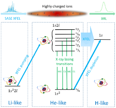
Figure 1: Scheme of the lasing process. An upper lasing state $1s2l$ of He-like ions is pumped through K-shell photoionization of Li-like ions initially in a $1s^{2}2l$ state by an XFEL pulse tuned above the K-edge of the He-like ions (blue arrow left). Lasing takes place through one of the four possible transitions from an upper lasing state $1s2l$ to the lower lasing state $1s^{2}$ (green arrows). The state $1s^{2}$ is depleted through further K-shell photoionization by the same XFEL pulse (blue arrow right). L-shell photoionization of the upper lasing states is represented by the thick blue arrow. The order of the $1s2l$ states may vary for different elements.

Plasma-based XRLs have achieved saturated amplification for different wavelengths in the soft-x-ray regime. Such lasers are mainly based on the $3p\rightarrow 3s$ or $4d\rightarrow 4p$ transition in Ne- or Ni-like ions for elements varying from ¹⁴Si to ⁷⁹Au, where the population inversion is achieved through electron collisional excitation in a hot dense plasma ^{21; 22}. The first hard-XRL was initially proposed through direct pumping of the $1s^{-1}\rightarrow 2s^{-1}$ transition via photoionization of a K-shell electron ²³. Limited by the high pump power required, this scheme was demonstrated only in recent years after high-flux XFELs became available ^{6; 7}. In the experiments with solid copper, an XRL at 1.54 Å was obtained, with a measured relative bandwidth of $2\times 10^{-4}$ determined by the short lifetime of the upper lasing state due to fast Auger decay. Here we put forward an XFEL-pumped transient XRL based on He-like HCIs, where the detrimental Auger-decay channel is nonexistent due to the lack of outer-shell electrons. By choosing a lasing transition which slowly decays radiatively, this results in a further reduction of the XRL bandwidth by several orders of magnitude.

Table 1: Results for selected x-ray lasing transitions for different elements. Radiative parameters like transition energy $\omega_{\text{0}}$, natural linewidth $\Gamma$ and upper-state lifetime $\tau$ are obtained from the GRASP code ²⁴. The XFEL photon energy $\omega_{\text{xfel}}$, tuned above the K-shell ionization threshold of the $1s^{2}$ state, and the mean peak flux (ph. stands for photons), used in the 1,000 realizations of the SASE XFEL pulses, are fixed to ensure population inversion and the applicability of the two-level approximation. Electron temperature $T_{\text{e}}$ and ion density $N_{\text{i}}$ ($n_{\text{0}}=10^{20}\text{ cm}^{-3}$) are chosen to enable a significant fraction of Li-like ions in the plasma ²⁵ (Supplementary Fig. S1). The broadening effects, with Doppler broadening $\Delta\omega_{\text{D}}$, electron–ion impact broadening $\Delta\omega_{\text{e-i}}$, and ion–ion Stark broadening $\Delta\omega_{\text{i-i}}$, are calculated for given $T_{\text{e}}$ and $N_{\text{i}}$ based on Maxwell–Boltzmann distributions ²⁶, with ion temperature $T_{\text{i}}=487$ K. The characteristic length $L_{\text{c}}$ is the optimal length defined in Fig. 2. The XRL intensity $I_{\text{c}}$ as well as the relative bandwidth $\Delta\omega/\omega_{0}$ at this length are obtained by averaging over 1,000 simulations, with the uncertainties arising from the random XFEL pulse profile. The upper and lower bounds are the values at the 10th and 90th percentiles of the corresponding distributions (as shown in Figs. 2d,f for $\text{Ar}^{\text{16+}}\leavevmode\nobreak\ {}^{3}P_{1}$).

Radiative parameters				XFEL		Plasma conditions					Simulation results
Upper state	$\omega_{\text{0}}$	$\Gamma$	$\tau$	$\omega_{\text{xfel}}$	peak flux	$T_{\text{e}}$	$N_{\text{i}}$	$\Delta\omega_{\text{D}}$	$\Delta\omega_{\text{e-i}}$	$\Delta\omega_{\text{i-i}}$	$L_{\text{c}}$	$I_{\text{c}}$	$\Delta\omega/\omega_{0}$
$1s2l$	(keV)	(meV)	(ps)	(keV)	(ph./cm2/s)	(keV)	($n_{\text{0}}$)	(meV)	(meV)	(meV)	(mm)	$\text{(W}/\text{cm}^{2}\text{)}$
$\text{Ne}^{\text{8+}}\leavevmode\nobreak\ {}^{1}P_{1}$	$0.920$	$6.08$	$0.10$	1.197	$1.10\times 10^{34}$	0.035	$0.02$	3.23	0.08	0.06	2.8	$4.5\begin{subarray}{c}{}_{+9.3}\\ {}^{-4.4}\end{subarray}\times 10^{12}$	$7.8\begin{subarray}{c}{}^{+4.3}\\ {}^{-2.7}\end{subarray}\times 10^{-5}$
$\text{Ar}^{\text{16+}}\leavevmode\nobreak\ {}^{3}P_{1}$	$3.120$	$1.16$	$0.57$	4.124	$2.29\times 10^{33}$	0.25	$0.25$	7.80	1.38	9.81	3.3	$5.0\begin{subarray}{c}{}_{+3.8}\\ {}^{-4.0}\end{subarray}\times 10^{14}$	$7.8\begin{subarray}{c}{}^{+1.9}\\ {}^{-2.1}\end{subarray}\times 10^{-6}$
$\text{Ar}^{\text{16+}}\leavevmode\nobreak\ {}^{1}P_{1}$	$3.137$	$72.2$	$0.009$	4.124	$1.98\times 10^{35}$	0.25	$2.48$	7.83	0.29	25.22	0.35	$1.5\begin{subarray}{c}{}_{+1.4}\\ {}^{-0.8}\end{subarray}\times 10^{16}$	$4.7\begin{subarray}{c}{}^{+2.0}\\ {}^{-1.7}\end{subarray}\times 10^{-5}$
$\text{Kr}^{\text{34+}}\leavevmode\nobreak\ {}^{3}P_{2}$	$13.087$	$0.07$	$9.46$	17.316	$1.87\times 10^{34}$	6.20	$0.50$	22.58	0.45	2.76	289	$4.3\begin{subarray}{c}{}_{+7.6}\\ {}^{-4.2}\end{subarray}\times 10^{16}$	$3.7\begin{subarray}{c}{}^{+1.6}\\ {}^{-1.1}\end{subarray}\times 10^{-7}$
$\text{Xe}^{\text{52+}}\leavevmode\nobreak\ {}^{3}P_{2}$	$30.589$	$1.91$	$0.34$	40.304	$7.45\times 10^{34}$	25.00	$27.0$	42.16	7.60	126	8.5	$4.7\begin{subarray}{c}{}_{+6.9}\\ {}^{-4.5}\end{subarray}\times 10^{18}$	$1.5\begin{subarray}{c}{}^{+0.6}\\ {}^{-0.5}\end{subarray}\times 10^{-6}$

The photoionization-pumped atomic laser is illustrated in Fig. 1, where the Li-like HCIs are initially prepared in a $1s^{2}2l$ ($l=s,p$) state in a laser-produced plasma ²⁵. A SASE XFEL pulse tuned above the K-edge of the ions first removes a K-shell electron from the Li-like ions, creating He-like ions in the $1s2l$ excited states. Subsequent decay to the $1s^{2}$ ground state leads to emission of x-ray photons via four possible K$\alpha$ transitions: one magnetic-dipole ($M1$) transition from the ${}^{3}S_{1}$ state, two electric-dipole ($E1$) transitions from the ${}^{3}P_{1}$ or ${}^{1}P_{1}$ states, and one magnetic-quadrupole ($M2$) transition from the ${}^{3}P_{2}$ state. The population inversion in the He-like ions resulting from this photoionization-pumping scheme leads to amplification of the emitted x-rays, i.e., to inner-shell x-ray lasing.

Two factors determine which transition will lase. Firstly, population inversion is needed to have stimulated emission. Typical XFEL facilities, with peak photon fluxes of $10^{33}$ – $10^{35}\text{\leavevmode\nobreak\ cm}^{-2}\text{\leavevmode\nobreak\ s}^{-1}$ (1 $\mu$m² spot size, ref. (17; 19)), yield an inverse ionization rate of a few femtoseconds, such that XFEL pulses can effectively photoionize all the Li-like ions. Transitions with upper-state lifetimes longer than 1 fs are necessary to ensure population inversion between the $1s2l$ and $1s^{2}$ state. Furthermore, the finite lifetime of the plasma $\tau_{\text{p}}\sim 10$ ps (ref. (27)) also influences the lasing process. Sufficient amplification of x-ray radiation will take place only from transitions whose decay is slower than XFEL pumping, but faster than plasma expansion.

Suitable XRL transitions in He-like ions are shown in table 1. Simulations for each transition have been conducted by solving the Maxwell–Bloch equations ^{28; 29} (Supplementary Information) numerically in retarded-time coordinates for 1,000 different realizations of SASE XFEL pulses. For most of the ions displayed in table 1, only one of the four transitions in Fig. 1 satisfies the requirements for lasing described above, such that a two-level description of the He-like ions is applicable. For $\text{Ar}^{\text{16+}}$ ions, there are two transitions which may lase simultaneously. Thus, the XFEL peak flux is tuned properly to ensure that only one of them lases. Values of the initial populations of the states in Li- and He-like ions are computed with the FLYCHK code ²⁵. XFEL frequencies and photon fluxes are then fixed such that K-shell photoionization of the $1s^{2}2l$ and $1s^{2}$ states ensures population inversion in the He-like ions (Supplementary Information). Except for the transition from $\text{Kr}^{\text{34+}}\leavevmode\nobreak\ {}^{3}P_{2}$, which needs more than 10 cm to reach saturated intensity, all the other transitions are predicted to generate high-intensity x-ray pulses within 1 cm with small bandwidths. For $E1$ transitions in $\text{Ne}^{\text{8+}}$ and $\text{Ar}^{\text{16+}}$, a significant improvement of $\Delta\omega/\omega$ is obtained compared to SASE XFEL pulses ¹⁷ and XRLs with neutral atoms ^{6; 7}. When going to heavier $\text{Kr}^{\text{34+}}$ and $\text{Xe}^{\text{52+}}$ ions, the $M2$ transitions provide an even more significant reduction of the bandwidth, with $\Delta\omega/\omega_{0}$ being $3.7\times 10^{-7}$ and $1.5\times 10^{-6}$, respectively. The resulting $13$- and $30$-keV lasers feature similar bandwidths as the untested XFELO scheme ⁸, with intensities of $\sim 10^{18}\text{\leavevmode\nobreak\ W\leavevmode\nobreak\ cm}^{-2}$. The relative bandwidths are by 2 to 3 orders of magnitude narrower than the value predicted for future seeded-XFEL sources at analogous hard-x-ray wavelengths around 0.41 – 0.95 Å (ref. (17)).

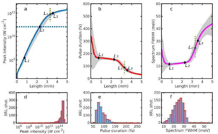
Figure 2: Evolution of the XRLs over 1,000 simulations ($\text{Ar}^{\text{16+}}\leavevmode\nobreak\ {}^{3}P_{1}$). a-c, Peak intensity, pulse duration and spectral full width at half maximum (FWHM) for the x-ray laser. The solid lines display results averaged over 1,000 simulations. The dotted line in (a) indicates the saturation intensity $I_{\text{s}}=1.18\times 10^{12}\text{\leavevmode\nobreak\ W\leavevmode\nobreak\ cm}^{-2}$. $L_{1}$, $L_{2}$ and $L_{3}$ mark the lengths for the XRL pulse to reach transform-limited profile, saturation intensity and Rabi flopping, respectively. $L_{\text{c}}$ refers to the characteristic length that optimizes the intensity and bandwidth of the XRL pulses. Here, it is defined as the length at which the slope of the solid line in (a) is 1/3 of the slope at $L_{2}$. The gray areas in (a-c) indicate the distribution areas of the results over 1,000 simulations. At a given length, the bottom and top edges of the areas indicate the 10th and 90th percentiles of the distributions, respectively. d-f, Distributions of the peak intensity, pulse duration and spectral FWHM at $L_{\text{c}}$ along the green dotted lines in (a-c). In (d), there are 15 simulations whose peak intensities locate in the unsaturated region $10^{6}\sim 10^{12}\text{\leavevmode\nobreak\ W\leavevmode\nobreak\ cm}^{-2}$, indicating that 1.5% of the SASE XFEL pulses cannot provide enough pumping.

To understand the properties of our XRLs and how they develop in the plasma, simulation results for the ${}^{3}P_{1}\rightarrow\leavevmode\nobreak\ ^{1}S_{0}$ transition in Ar¹⁶⁺ are shown in Figs. 2 and 3 for the corresponding parameters listed in table 1. We use a partial-coherence method ³⁰ to simulate $124$-fs-long SASE XFEL pulses with a spectral width of $1.55$ eV and peak photon flux of $2.29\times 10^{33}\text{\leavevmode\nobreak\ cm}^{-2}\text{\leavevmode\nobreak\ s}^{-1}$. This results in a peak pumping rate of $6.04\times 10^{13}\text{\leavevmode\nobreak\ s}^{-1}$ for the upper lasing state, and a depletion rate of $5.63\times 10^{13}\text{\leavevmode\nobreak\ s}^{-1}$ for the lower lasing state. They are $32$ and $58$ times larger than the spontaneous-emission rate of the ${}^{3}P_{1}$ state, ensuring population inversion.

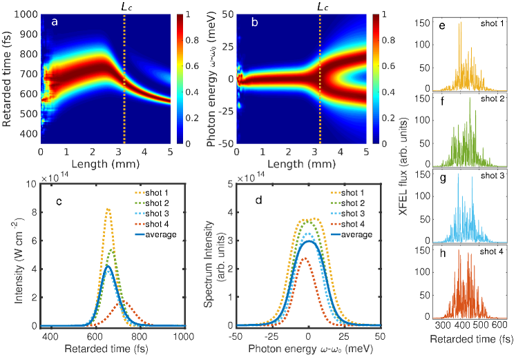
Figure 3: Evolution of the normalized XRL intensity and spectrum ($\text{Ar}^{\text{16+}}\leavevmode\nobreak\ {}^{3}P_{1}$, single simulation). a, Intensity shown as a function of retarded time and propagation length. b, Power spectrum displayed as a function of photon energy and propagation length. For a given length, the intensity and spectrum are normalized to the maximum value of the corresponding profiles at that length. The vertical dotted lines indicate the characteristic length $L_{\text{c}}$ shown in Fig. 2. For lengths larger than $L_{\text{c}}$, the strength of the second peak in (a) appearing around retarded times of $\sim 700$ fs has been multiplied by a factor of 5 for better visibility. c,d, XRL pulse profile and spectrum at $L_{\text{c}}$. The yellow dotted lines correspond to the results from the simulation in (a,b). Three other simulation results (green, blue and red dotted lines) at $L_{\text{c}}$ are also included for comparison, with the solid lines corresponding to the results averaged over 1,000 simulations. e-h, SASE XFEL pulses used in the four simulations in (c,d). Differences in amplitudes and positions of the peak intensities in (c,d) are the result of shot-to-shot random profiles of the SASE XFEL pulses. XRL intensity and spectrum as a function of propagation length for the XFEL pulses in (f-h), and averaged over 1,000 simulations, can be found in the Supplementary Information. In (c,d), the blue solid lines are obtained by averaging XRL pulse shapes and spectra as a function of retarded time and frequency, respectively. The peak intensity of the averaged XRL pulse shape in (c), therefore, differs from the averaged value of the XRL peak intensity displayed in Fig. 2a and table 1, because the position of the intensity peak varies from shot to shot.

Average results over 1,000 SASE-pulse realizations are shown in Figs. 2a-c. The peak intensity of the XRL, shown by the solid line in Fig. 2a, increases exponentially during the initial propagation stage, then displays a saturation behavior. The dotted line indicates the saturation intensity $I_{\text{s}}=\hbar\Gamma\omega_{0}^{3}/6\pi c^{2}$ at which the stimulated-emission rate equals the spontaneous-emission rate. This is also the intensity from which the amplification begins to slow down. The evolution of the pulse duration and the spectral width are shown by the solid lines in Figs. 2b,c. At $L=0$, only spontaneous emission takes place: the 342-fs average pulse duration is mainly determined by the lifetime of the ${}^{3}P_{1}$ state (Fig. 2b), whereas the 23.5-meV intrinsic spectral width before propagation (Fig. 2c) is mostly due to the sum of the natural linewidth $\Gamma$ and the three broadening effects shown in table 1.

During its propagation in the medium, gain narrowing and saturation rebroadening will also contribute to the final bandwidth. This can be observed by inspecting the four distinct propagation regions separated by $L_{1}$, $L_{2}$ and $L_{3}$ in Figs. 2a-c, which can also be followed in Figs. 3a,b for a single simulation. Up to $L_{1}=0.75$ mm, both the pulse duration and spectral FWHM decrease severely. The laser intensity and spectrum in this region for a single simulation are spiky and noisy, as the ions irradiate randomly in time and space (Figs. 3a,b). When the spontaneously emitted signal propagates and stimulated emission sets in, it selectively amplifies the frequencies around $\omega_{0}$ such that the XRL pulse approaches a fully coherent transform-limited profile at $L_{1}$ (ref. (29)), with a bandwidth smaller than the intrinsic width. Thereafter, a gradual broadening of the spectrum is observed in the region $L_{1}L_{2}$. The broadening increases abruptly from $L_{2}=2.3$ mm, where the saturation intensity has been reached and the stimulated-emission rate exceeds the spontaneous-emission rate. This is accompanied by a substantial slowing down of the amplification of the intensity and a significant decrease of the pulse duration in the region between $L_{2}$ and $L_{3}$ (Figs. 2a,b). Further propagation of the XRL pulse after $L_{3}=3.5$ mm is characterized by the onset of Rabi flopping (Fig. 3a) which is reflected by a splitting in the XRL spectrum (Fig. 3b). This effect is much stronger and more marked than for previous XFEL-pumped transient lasers with neutral atoms (ref. (29)) due to the absence of Auger decay ³⁰. At the same time, the gain of the laser intensity in this region is strongly suppressed.

The optimal choice for a coherent XRL pulse is located in the third region $L_{2}L_{3}$, where saturation has already been reached while the bandwidth is still narrow. By choosing the medium length to be $L_{\text{c}}=3.3$ mm, as shown in Fig. 2, one will obtain an approximately $87$-fs-long XRL pulse with an average peak intensity of $I_{\text{c}}=5.0\times 10^{14}\text{\leavevmode\nobreak\ W\leavevmode\nobreak\ cm}^{-2}$ ($\sim$80% fluctuations) and an average bandwidth of $\Delta\omega=24.5$ meV ($\sim$30% fluctuations) (table 1). This gives $\Delta\omega/\omega_{0}=7.8\times 10^{-6}$ for a total of $6.5\times 10^{8}$ coherent photons, with a peak brilliance of $1.4\times 10^{31}$ photons/s/mm²/mrad²/0.1%bandwidth.

In conclusion, we put forward a scheme to obtain high-intensity x-ray lasers with bandwidths up to three orders of magnitude narrower compared to the value predicted for seeded-XFEL sources in the hard-x-ray regime ¹⁷. While the photon energies of the XRLs are fixed by the corresponding isolated transitions, three-wave interactions by synchronizing XFEL pulses with optical/XUV lasers could be investigated in future studies to tune the frequencies in a broad range. Such x-ray sources will enable novel studies of coherent light–matter interactions in atomic, molecular and solid-state systems.

The authors thank S. Tang, Y. Wu and J. Gunst for fruitful discussions. C.L. developed the mathematical model, performed the analytical calculations and numerical simulations, and wrote the manuscript. S.M.C. and Z.H. conceived the underlying scheme. All authors contributed to the development of ideas, discussion of the technical aspects and results, and preparation of the manuscript. Correspondence and requests for materials should be addressed to S.M.C. (smcavaletto@gmail.com).

Supplementary Information

A Modeling of the propagation through the medium

In this section, we first discuss the model used to describe lasing in He-like ions in the two-level approximation. Maxwell–Bloch equations are developed to model the dynamics of the system and the propagation of the x-ray laser (XRL) pulse through the gain medium. The equations are solved numerically with a Runge–Kutta method in the retarded time domain. Initial populations of the ionic states are obtained from FLYCHK simulations of the charge-state distributions under given plasma conditions. Cross sections of XFEL photoionization for each element, as well as XFEL pulse durations and bandwidths used in the simulations, are also listed.

A1 Maxwell–Bloch equations in the two-level approximation

Selected transitions applicable for our lasing scheme are shown in table 1 from the main text. A full description of the lasing process should account for all the $1s2l$ ($l=s,p$) states in He-like ions. However, the lifetimes of these states differ from each other by orders of magnitude. When only one of the four K$\alpha$ transitions in the He-like ions satisfies the lasing requirements described in the main text, a two-level description of the ions is sufficient.

For light ions, Ne⁸⁺ for example, the $E1$ transition with a decay rate of $9.24\times 10^{12}\text{ s}^{-1}$ from the ${}^{1}P_{1}$ state will develop lasing. The other transitions have decay times much larger than the plasma expansion time, and their contribution is negligible compared to the ${}^{1}P_{1}$ state, such that they can be neglected. For heavy ions like Xe⁵²⁺, however, the two $E1$ transition rates scale as $\sim Z^{4}$ ($Z$ being the atomic number), corresponding to $3.05\times 10^{15}\text{ s}^{-1}$ for ${}^{3}P_{1}$ and $6.82\times 10^{15}\text{ s}^{-1}$ for ${}^{1}P_{1}$, respectively, which are too large to enable population inversion with available XFEL pulses. On the other hand, the decay rate of the $M1$ transition from the ${}^{3}S_{1}$ state and the $M2$ transition from the ${}^{3}P_{2}$ state are $3.7\times 10^{11}\text{ s}^{-1}$ and $2.56\times 10^{12}\text{ s}^{-1}$, respectively, which are sufficient for lasing to take place before the expansion of the plasma. However, the $M1$ transition from the ${}^{3}S_{1}$ state is dominated by large Stark broadening effects, such that the amplification of photons emitted from such transition is much slower than for those emitted in the $M2$ transition. Within the characteristic length $L_{\text{c}}$ for the $M2$ transition, the presence of the ${}^{3}S_{1}$ state can hence be neglected. Similar arguments are applicable to Kr³⁴⁺.

For $\text{Ar}^{\text{16+}}$, there are two transitions that may lase simultaneously, as listed in table 1 from the main text. However, the lifetimes $\tau$ of these states differ from each other by a factor of 63. The XFEL photon flux can be tuned properly to exclude one of them from lasing. For instance, in order to obtain lasing from the ${}^{3}P_{1}\rightarrow\leavevmode\nobreak\ ^{1}S_{0}$ transition, a mean peak flux of $2.29\times 10^{33}\text{ cm}^{-2}\text{ s}^{-1}$ for the XFEL pulses is applied. This generates an upper state pumping rate and a lower-state depletion rate which are $32$ and $58$ times larger than the decay rate of the ${}^{3}P_{1}$ upper state, respectively, resulting in population inversion of the transition. At the same time, for this value of the peak flux, the pumping rate of the ${}^{1}P_{1}$ upper state is only 0.26 times the decay rate of the ${}^{1}P_{1}$ state, too small to obtain population inversion in the ${}^{1}P_{1}\rightarrow\leavevmode\nobreak\ ^{1}S_{0}$ transition. Thereby, lasing will only take place from the ${}^{3}P_{1}$ state. Sufficient amplification of the x-ray photons emitted from the ${}^{1}P_{1}$ state needs higher XFEL peak fluxes and higher ion densities. When such conditions are met, e.g., for the parameters shown in table 1 in the main text, lasing from the ${}^{1}P_{1}\rightarrow\leavevmode\nobreak\ ^{1}S_{0}$ transition takes place. Saturation will be reached much sooner than for the ${}^{3}P_{1}\rightarrow\leavevmode\nobreak\ ^{1}S_{0}$ transition, such that the ${}^{3}P_{1}$ state can be neglected.

Assuming XFEL pulses propagating along the $\hat{x}$ direction, the evolution of the x-ray laser field in the slowly varying envelope approximation is given by ^{2; 1}

$$\frac{\partial\mathcal{A}(x,t)}{\partial t}+c\frac{\partial\mathcal{A}(x,t)}{\partial x}=i\frac{\mu_{\text{0}}\omega_{\text{0}}c^{2}}{2}\mathcal{F}(x,t),$$ (S1)

where $\mathcal{A}(x,t)$ is either the electric field $\mathcal{E}(x,t)$ or the magnetic field $\mathcal{B}(x,t)$, depending on the specific transition. $\mu_{\text{0}}$ is the vacuum permeability and $c$ is the vacuum speed of light. $\mathcal{F}(x,t)$ corresponds to the polarization field induced by $\mathcal{E}(x,t)$ for $E1$ transitions, or the magnetization field and magnetic-quadrupole field induced by $\mathcal{B}(x,t)$ for $M1$ transitions and $M2$ transitions, respectively.

For a given lasing transition, we assume all Li-like ions are pumped into the corresponding upper lasing state of such transition by the XFEL pulse. Using $\left|\text{e}\right>$ and $\left|\text{g}\right>$ to represent the upper lasing state and the lower lasing state, respectively, the dynamics of the He-like ions are described by the Bloch equations of the density matrix

$$\dot{\rho}_{\text{ee}}(x,t) = -\text{Im[}\Omega^{*}(x,t)\rho_{\text{eg}}(x,t)\text{]}+\sigma_{\text{0}}j_{\text{xfel}}(x,t)\rho_{\text{00}}(x,t)-\sigma_{\text{e}}j_{\text{xfel}}(x,t)\rho_{\text{ee}}(x,t)-\Gamma\rho_{\text{ee}}(x,t),$$ (S2)

$$\dot{\rho}_{\text{eg}}(x,t) = \frac{i}{2}\Omega^{*}(x,t)(\rho_{\text{ee}}(x,t)-\rho_{\text{gg}}(x,t))-\frac{\gamma}{2}\rho_{\text{eg}}(x,t)+S(x,t),$$ (S3)

$$\dot{\rho}_{\text{gg}}(x,t) = \text{Im[}\Omega^{*}(x,t)\rho_{\text{eg}}(x,t)\text{]}-\sigma_{\text{g}}j_{\text{xfel}}(x,t)\rho_{\text{gg}}(x,t)+\Gamma\rho_{\text{ee}}(x,t).$$ (S4)

The carrier frequency $\omega_{\text{0}}$ is chosen to be resonant with the lasing transition. $\rho_{\text{ee}}$ and $\rho_{\text{gg}}$ are the populations of $\left|\text{e}\right>$ and $\left|\text{g}\right>$, and the off-diagonal term $\rho_{\text{eg}}$ represents the coherence between the two lasing states. $\Omega(x,t)=\wp\mathcal{E}(x,t)/\hbar$ for an $E1$ transition (or $\Omega(x,t)=m\mathcal{B}(x,t)/\hbar$ for an $M1$ transition, and $\Omega(x,t)=k_{0}q_{yx}\mathcal{B}(x,t)/\hbar$ for an $M2$ transition ³) is the time- and space-dependent Rabi frequency, with $\wp$ the electric-dipole moment, $m$ the magnetic-dipole moment, and $q_{yx}$ the $yx$-component of the magnetic-quadrupole tensor. XFEL pumping of the $\left|\text{e}\right>$ state from Li-like ions is accounted for through the second term in the right-hand side of Eq. (S2), with $\rho_{\text{00}}$ being the population of Li-like ions, $j_{\text{xfel}}$ the photon flux of the XFEL pump pulse, and $\sigma_{\text{0}}$ the K-shell photoionization cross section of the pump process ($1s^{2}2l\rightarrow 1s2l$). The XFEL pulse also depletes the $\left|\text{e}\right>$ and $\left|\text{g}\right>$ states, as modeled by the third term on the right-hand side of Eq. (S2) and the second term on the right-hand side of Eq. (S4), respectively, with $\sigma_{\text{e}}$ and $\sigma_{\text{g}}$ being the corresponding photoionization cross sections. In Eqs. (S2) and (S4), $\Gamma\rho_{\text{ee}}(x,t)$ describes spontaneous emission at rate $\Gamma$. In Eq. (S3), the parameter

$$\gamma=\Gamma+\Delta\omega_{\text{e-i}}+(\sigma_{\text{e}}+\sigma_{\text{g}})j_{\text{xfel}}(x,t)$$ (S5)

models the three contributions to the decay of the off-diagonal elements: $\Gamma$ is the decoherence originating from spontaneous photon emission; the second term $\Delta\omega_{\text{e-i}}$ accounts for the broadening from electron–ion collisions ⁵; and the final term describes the contribution from depletion of the total population of He-like ions. $S(x,t)$ in Eq. (S3) is a Gaussian white-noise term added phenomenologically, which satisfies $\left<S^{*}(x,t)S(z,t^{\prime})\right>=F(z,t_{1})\delta(t-t^{\prime})$. For $E1$ transitions, one has ²

$$F(x,t) = \frac{\varepsilon_{0}\hbar\omega_{0}}{N_{\text{i}}\wp^{2}}\frac{d}{8\pi L}\frac{\gamma^{2}}{\omega_{0}^{2}}\Gamma\rho_{\text{ee}}(x,t),$$ (S6)

where $\varepsilon_{0}$ is the vacuum permittivity and $N_{\text{i}}$ stands for the density of the ions in the plasma. $d=0.4$ $\mu$m is the radius of the XFEL spot on the plasma and $L$ is the length of the plasma.

The coupling between the Maxwell equations and the Bloch equations is given through the induced fields $\mathcal{P}=-2N_{\text{i}}\wp\rho_{\text{eg}}$, $\mathcal{M}=-2N_{\text{i}}m\rho_{\text{eg}}$ and $\mathcal{Q}=-2N_{\text{i}}q\rho_{\text{eg}}$ for $E1$, $M1$, and $M2$ transitions, respectively. Absorption of the XFEL pulse by the ions is included through the rate equations

$$\frac{\partial j_{\text{xfel}}}{\partial z}=-\sum_{\text{k}}\sigma_{\text{k}}\rho_{\text{kk}}N_{\text{i}}j_{\text{xfel}},$$ (S7)

where k={0, e, g} represents the three different states.

A2 Charge-state distribution

Values of the initial populations of the states in Li- and He-like ions are computed with the FLYCHK code ⁴

$$\rho_{\text{00}}(x,t=0) = \rho_{{}_{\text{Li-like}}},$$ (S8)

$$\rho_{\text{ee}}(x,t=0) = 0,$$ (S9)

$$\rho_{\text{gg}}(x,t=0) = \rho_{{}_{\text{He-like}}},$$ (S10)

where $\rho_{{}_{\text{Li-like}}}$ and $\rho_{{}_{\text{He-like}}}$ are the fractions of Li-like ions ($1s^{2}2l$ state) and He-like ions ($1s^{2}$ state) shown in Fig. S1. The initial population of the $1s2l$ upper lasing states in He-like ions is found to be negligible. Thus, most of the He-like ions are in the lower lasing state and no population inversion exists before XFEL-pulse pumping sets in. Since the decay of the upper lasing state in He-like ions is much slower than the K-shell photoionization rate, after the Li-like ions are pumped to a $1s2l$ state, this decays on a time scale much longer than the inverse of the K-shell photoionization rate. Population inversion develops after the lower lasing state ($1s^{2}$) of the He-like ions has been depleted by the XFEL pulse. In the simulation, only evolutions of the He-like ions are described by density-matrix theory. The evolution of the populations of the other charge states is modeled through rate equations.

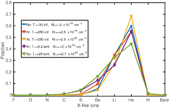
Figure S1: Charge-state distributions for different elements and simulation parameters.

A3 XFEL parameters

Using the radiative parameters displayed in table 1 from the main text, and the corresponding K-shell and L-shell photoionization cross sections shown in table S1, the XFEL parameters are fixed such that the requirements for lasing described in the main text and in Sec. A1 are satisfied, and significant population inversion can be obtained. In particular, the XFEL photon energies $\omega_{\text{xfel}}$ listed in table 1 in the main text are tuned above the K-edge of the He-like ions, in order to ensure depletion of the initial population in the lower lasing state of He-like ions. For the elements considered, this photon energy is also above the K-edge of the corresponding Li-like ions. Photoionization of Li-like ions to a $1s2l$ excited state in He-like ions then ensures population inversion of the considered lasing transition. Most of the XFEL bandwidths listed in table S1 are chosen taking into account realistic parameters at XFEL facilities in operation or under construction. Only for the case of $\text{Kr}^{\text{34+}}$ and $\text{Xe}^{\text{52+}}$, the smallest values of the XFEL coherence times, thus the largest values of the XFEL bandwidths, used in the simulations are limited by the time steps ($\delta t=0.0001\tau=0.95$ fs for $\text{Kr}^{\text{34+}}$ and $\delta t=0.001\tau=0.34$ fs for $\text{Xe}^{\text{52+}}$) employed in our numerical calculations of the Maxwell–Bloch equations. However, simulations run with smaller time steps, thus larger XFEL bandwidths, provide results which are not significantly different. This is because photoionization pumping is determined by the XFEL flux and is not significantly influenced by the properties of the XFEL spectrum ¹. Therefore, when we compare the bandwidth of the XRLs and XFEL pulses in the main text, we refer to the realistic bandwidth measured at XFEL facilities and not to the values used in this table.

Table S1: Extended XFEL parameters. K-shell ionization cross section $\sigma_{\text{0}}$ and $\sigma_{\text{g}}$, together with the L-shell ionization cross section $\sigma_{\text{e}}$, are calculated from the LANL Atomic Physics Codes ⁸ ($\text{kb}=10^{-21}\text{ cm}^{2}$). SASE XFEL parameters such as pulse duration, bandwidth and total photons inserted into the medium are simulated with a partial-coherence method ⁹. The number of photons absorbed during the lasing process is obtained from our numerical solutions of Eqs. (S2 – S7).

XFEL ionization cross section				XFEL parameters
Upper state	$\sigma_{\text{0}}$	$\sigma_{\text{e}}$	$\sigma_{\text{g}}$	duration	bandwidth	photons inserted	photons absorbed
$1s2l$	(kb)	(kb)	(kb)	(fs)	(eV)
$\text{Ne}^{\text{8+}}\leavevmode\nobreak\ {}^{1}P_{1}$	$39.1$	$1.6$	$151.2$	21.3	$6.25$	$2.4\times 10^{12}$	$6.3\times 10^{9}$
$\text{Ar}^{\text{16+}}\leavevmode\nobreak\ {}^{3}P_{1}$	$24.6$	$0.48$	$44.6$	124	$1.55$	$2.9\times 10^{12}$	$1.0\times 10^{12}$
$\text{Ar}^{\text{16+}}\leavevmode\nobreak\ {}^{1}P_{1}$	$12.4$	$0.47$	$44.6$	2.0	$74$	$3.8\times 10^{12}$	$2.7\times 10^{10}$
$\text{Kr}^{\text{34+}}\leavevmode\nobreak\ {}^{3}P_{2}$	$6.24$	$0.12$	$10.9$	202	$0.57$	$3.9\times 10^{13}$	$2.0\times 10^{13}$
$\text{Xe}^{\text{52+}}\leavevmode\nobreak\ {}^{3}P_{2}$	$2.66$	$0.06$	$5.31$	72.5	$1.96$	$5.6\times 10^{13}$	$3.6\times 10^{13}$

B Line broadening in plasma

In the following, we explain in detail the role of the presence of Doppler, collisional and Stark broadening effects, as they are also comparable to the relatively small natural linewidth. As shown in table 1 from the main text, the Doppler broadening

$$\Delta\omega_{\text{D}}=\sqrt{\frac{8\text{ln}2k_{\text{B}}T_{\text{i}}}{m_{\text{i}}c^{2}}}\omega_{\text{0}},$$ (S11)

with $k_{\text{B}}$ being the Boltzmann constant, $T_{\text{i}}$ the ion temperature and $m_{\text{i}}$ the mass of the He-like ions, is not significant for light ions, but it becomes dominant for heavy ions like $\text{Kr}^{\text{34+}}$ and $\text{Xe}^{\text{52+}}$.

The electron-impact broadening is given by ⁵

$$\Delta\omega_{\text{e-i}} = -\frac{16}{3\bar{v}_{\text{e}}}\frac{N_{\text{e}}\hbar^{2}}{Z_{\text{i}}^{2}m_{\text{e}}^{2}}\text{ln}\Lambda\leavevmode\nobreak\ \left<\bm{r}\bm{r}\right>,$$ (S12)

with $\bar{v}_{\text{e}}=\sqrt{8k_{\text{B}}T_{\text{e}}/\pi m_{\text{e}}}$ being the average thermal velocity of the electrons in the plasma and $N_{\text{e}}$ the electron density, and $Z_{\text{i}}$ the charge number of the ions. $T_{\text{e}}$ and $m_{\text{e}}$ are the electron temperature and electron mass, respectively. $\text{ln}\Lambda\sim 10$ is the Coulomb logarithm and $\bm{r}\bm{r}$ is a tensor with $\bm{r}$ being the dipole operator of the bound electrons in the ions. Such broadening is significant only for light ions such as $\text{Ne}^{\text{8+}}$ and $\text{Ar}^{\text{16+}}$ with lower electron temperatures, but becomes negligible compared to $\Delta\omega_{\text{D}}$ for heavy ions and higher electron temperatures.

The quadratic Stark broadening from ion–ion interaction is calculated through ⁶

$$\Delta\omega_{\text{i-i}}=\alpha\overline{F^{2}},$$ (S13)

with

$$\alpha = -\frac{1}{4\pi\hbar}\sum_{k\neq j}\wp_{jk}^{2}/(eE_{kj}^{2}),$$ (S14)

$$\overline{F^{2}} = 4Z_{\text{p}}^{2}e^{2}N_{\text{i}}^{\frac{4}{3}}/(\pi\varepsilon_{0})^{2},$$ (S15)

$\alpha$ is the quadratic Stark coefficient which would be different for each transition, and $\overline{F^{2}}$ is the mean-square electric-field strength generated by nearby perturbing ions with charge number $Z_{\text{p}}$. $\wp_{jk}$ and $E_{jk}$ are the electric-dipole moment and energy difference between the states $\left|\text{j}\right>$ and $\left|\text{k}\right>$, respectively. $\Delta\omega_{\text{i-i}}$, in general, is negligible for $N_{\text{i}}<10^{19}$ cm^-3, but becomes large for dense ion gases.

In general, the natural broadening and electron–ion impact broadening are homogeneous for each ion, giving a Lorentzian spectrum. The Doppler broadening and ion–ion Stark broadening, on the other hand, are inhomogeneous for different ions, and result in a Gaussian spectrum. For systems involving both homogeneous and inhomogeneous broadenings, as it is the case here, the real spectrum has a Voigt line shape given by the convolution of the Lorentzian and Gaussian profiles, with a FWHM $\Delta\omega_{\text{V}}$ approximately given by ⁷

$$\Delta\omega_{\text{V}} = 0.5364\Delta\omega_{\text{L}}+\sqrt{0.2166\Delta\omega_{\text{L}}^{2}+\Delta\omega_{\text{G}}^{2}}.$$ (S16)

Here, $\Delta\omega_{\text{L}}=\Gamma+\Delta\omega_{\text{e-i}}$ is the FWHM of the Lorentzian function, and $\Delta\omega_{\text{G}}=\Delta\omega_{\text{D}}+\Delta\omega_{\text{i-i}}$ is the FWHM of the Gaussian function.

Numerical simulations of the lasing process accounting for the inhomogeneous broadening should take into account the distributions of the thermal velocity as well as Stark shift of the ions, which renders the simulations time consuming. However, Eq. (S16) shows that

$$\Delta\omega_{\text{V}}\sim\Delta\omega_{\text{L}}+\Delta\omega_{\text{G}}=\Gamma+\Delta\omega_{\text{e-i}}+\Delta\omega_{\text{D}}+\Delta\omega_{\text{i-i}}$$ (S17)

For the sake of simplicity, we can approximate the parameter in Eq. (S5) as

$$\gamma=\Gamma+\Delta\omega_{\text{e-i}}+\Delta\omega_{\text{D}}+\Delta\omega_{\text{i-i}}+(\sigma_{\text{e}}+\sigma_{\text{g}})j_{\text{xfel}}(x,t).$$ (S18)

With this approximation, the distribution of the ions over different thermal velocities and Stark shifts is automatically included in the Maxwell–Bloch equations. This simplification may lead to a maximum of 25% overestimate of the bandwidth compared to the Voigt bandwidth $\Delta\omega_{\text{V}}$ in the simulations. However, this will not change our conclusions in the main text.

C Other simulation results

Simulation results of the intensity profile and spectrum as a function of propagation length for shots 2–4 in Fig. 3 in the main text, as well as the intensity profile and spectrum averaged over 1,000 simulations, are displayed in Figs. S2–S4 and Fig. S5, respectively. Shot-to-shot differences are a consequence of the random SASE-XFEL-pulse profiles used, shown in Figs. 3e-f in the main text.

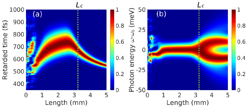
Figure S2: Evolution of the normalized x-ray laser intensity and spectrum (shot 2). Results for SASE-pulse shot 2 in Fig. 3f in the main text; green dotted lines in Figs. 3c,d in the main text. a, Intensity shown as a function of retarded time and propagation length. b, Power spectrum displayed as a function of photon energy and propagation length. For a given length, the intensity and spectrum are normalized to the maximum value of the corresponding profiles at such length. The vertical dotted lines indicate the characteristic length $L_{\text{c}}$ defined in the main text. The decrease in the XRL bandwidth at the end of the medium is a result of XFEL absorption.

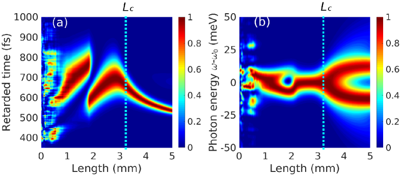
Figure S3: Same as Fig. S2 for shot 3. Results for SASE-pulse shot 3 in Fig. 3g in the main text; blue dotted lines in Figs. 3c,d in the main text. The exotic structures in both intensity and spectrum around $L=2$ mm originate from XFEL photoionization of the upper lasing state. The decay of this state is different during and after the XFEL pulse. This renders it possible that two peaks develop and propagate before saturation.

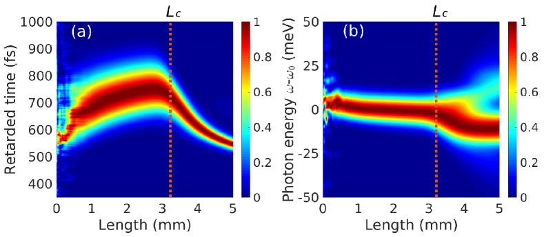
Figure S4: Same as Fig. S2 for shot 4. Results for SASE-pulse shot 4 in Fig. 3h in the main text; red dotted lines in Figs. 3c,d in the main text. A slight shift of the peak of the spectrum from $\omega_{0}$ is here apparent.

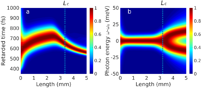
Figure S5: Evolution of the normalized x-ray laser intensity and spectrum averaged over 1,000 realizations of SASE XFEL pulses. Intensity and spectra evaluated at the characteristic length $L_{\text{c}}$ are exhibited by the solid lines in Figs. 3c,d in the main text. The chaotic features for small propagation lengths, which are shown for single simulations in Figs. 3a,b in the main text and in Figs. S2–S4 above, become smooth here.

References

- Lambert et al. (2008) Lambert G., et al. Injection of harmonics generated in gas in a free-electron laser providing intense and coherent extreme-ultraviolet light. Nature Phys. 4, 296 (2008).
- Amann et al. (2012) Amann J., et al. Demonstration of self-seeding in a hard-x-ray free-electron laser. Nature Photon. 6, 693 (2012).
- Allaria et al. (2012) Allaria E., et al. Highly coherent and stable pulses from the FERMI seeded free-electron laser in the extreme ultraviolet. Nature Photon. et al., Nature Photonics 6, 699 (2012).
- Ratner et al. (2015) Ratner D., et al. Experimental demonstration of a soft x-ray self-seeded free-electron laser. Phys. Rev. Lett. 114, 054801 (2015).
- Huang et al. (2017) Huang S., et al. Generating single-spike Hard x-ray pulses with nonlinear bunch compression in free-electron lasers. Phys. Rev. Lett. 119, 154801 (2017).
- Rohringer et al. (2012) Rohringer N., et al. Atomic inner-shell x-ray laser at 1.46 nanometres pumped by an x-ray free-electron laser. Nature 481, 488 (2012).
- Yoneda et al. (2015) Yoneda H., et al. Atomic inner-shell laser at 1.5-ångström wavelength pumped by an x-ray free-electron laser. Nature 524, 446 (2015).
- Kim et al. (2008) Kim K. J., Shvyd’ko Y. & Reiche S. A proposal for an x-ray free-electron laser oscillator with an energy-recovery linac. Phys. Rev. Lett. 100, 244802 (2008).
- Adams et al. (2013) Adams B. W., et al. X-ray quantum optics. J. Mod. Opt. 60, 2 (2013).
- Vagizov et al. (2014) \BibitemOpen\bibfieldauthor Vagizov F., Antonov V., Radeonychev Y., Shakhmuratov R. & Kocharovskaya O. Coherent control of the waveforms of recoilless -ray photons. \bibfieldjournal Nature 508, 80 (2014).
- Heeg et al. (2017) Heeg K. P., et al. Spectral narrowing of x-ray pulses for precision spectroscopy with nuclear resonances. Science 357, 375 (2017).
- Haber et al. (2017) Haber J., et al. Rabi oscillations of x-ray radiation between two nuclear ensembles. Nature Photon. 11, 720 (2017).
- Cavaletto et al. (2014) Cavaletto S. M., et al. Broadband high-resolution x-ray frequency combs. Nature Photon. 8, 520 (2014).
- Kanter et al. (2011) Kanter E. P., et al. Unveiling and driving hidden resonances with high-fluence, high-intensity x-ray pulses. Phys. Rev. Lett. 107, 233001 (2011).
- Doumy et al. (2011) Doumy G., et al. Nonlinear atomic response to intense ultrashort x rays. Phys. Rev. Lett. 106, 083002 (2011).
- Bernitt et al. (2012) Bernitt S., et al. An unexpectedly low oscillator strength as the origin of the FeXVII emission problem. Nature 492, 225 (2012).
- Pellegrini et al. (2016) Pellegrini C., Marinelli A., and Reiche S. The physics of x-ray free-electron lasers. Rev. Mod. Phys. 88, 015006 (2016).
- Bostedt et al. (2016) Bostedt C., et al. Linac Coherent Light Source: The first five years. Rev. Mod. Phys. 88, 015007 (2016).
- Seddon et al. (2017) Seddon E., et al. Short-wavelength free-electron laser sources and science: a review. Rep. Prog. Phys. 80, 115901 (2017).
- Rocca (1999) Rocca J. J. Table-top soft x-ray lasers. Rev. Sci. Instrum. 70, 3799 (1999).
- Daido (2002) Daido H. Review of soft x-ray laser researches and developments. Rep. Prog. Phys. 65, 1513 (2002).
- Suckewer and Jaegle (2009) Suckewer S. & Jaegle P. X-Ray laser: past, present, and future. Laser Phys. Lett. 6, 411 (2009).
- Duguay and Rentzepis (1967) Duguay M. & Rentzepis P. Some approaches to vacuum UV and x-ray lasers. Appl. Phys. Lett. 10, 350 (1967).
- Dyall et al. (1989) Dyall K., Grant I., Johnson C., Parpia F. & Plummer E. GRASP: A general-purpose relativistic atomic structure program. Comput. Phys. Commun. 55, 425 (1989).
- Chung et al. (2005) Chung H. K., Chen M., Morgan W., Ralchenko Y. & Lee R. FLYCHK: Generalized population kinetics and spectral model for rapid spectroscopic analysis for all elements. High Energy Density Phys. 1, 3 (2005).
- Griem (1974) Griem H. R. Spectral line broadening in plasmas. (Acadamic, New York, 1974).
- Krainov and Smirnov (2002) Krainov V. & Smirnov M. Cluster beams in the super-intense femtosecond laser pulse. Phys. Rep. 370, 237 (2002).
- Larroche et al. (2000) Larroche O. et al., Maxwell–Bloch modeling of x-ray-laser-signal buildup in single-and double-pass configurations. Phys. Rev. A 62, 043815 (2000).
- Weninger and Rohringer (2014) Weninger C. & Rohringer N. Transient-gain photoionization x-ray laser. Phys. Rev. A 90, 063828 (2014).
-
Cavaletto et al. (2012)
Cavaletto S. M.,
et al.
Resonance fluorescence in ultrafast and intense x-ray free-electron-laser pulses.
Phys. Rev. A
86,
033402 (2012).

References

- Weninger and Rohringer (2014) Weninger C. & Rohringer N. Transient-gain photoionization x-ray laser. Phys. Rev. A 90, 063828 (2014).
- Larroche et al. (2000) Larroche O. Maxwell–Bloch modeling of x-ray-laser-signal buildup in single-and double-pass configurations. et al., Phys. Rev. A 62, 043815 (2000).
- Pálffy et al. (2008) Pálffy A., Evers J. & Keitel C. H. Electric-dipole-forbidden nuclear transitions driven by super-intense laser fields. Phys. Rev. C 77, 044602 (2008).
- Chung et al. (2005) Chung H. K., Chen M., Morgan W., Ralchenko Y. & Lee R. FLYCHK: Generalized population kinetics and spectral model for rapid spectroscopic analysis for all elements. High Energy Density Phys. 1, 3 (2005).
- Griem and Shen (1961) Griem H. R. & Shen K. Y. Stark Broadening of Hydrogenic Ion Lines in a Plasma. Phys. Rev. 122, 1490 (1961).
- Griem (1974) Griem H. R. Spectral line broadening in Plasmas (Acadamic, New York, 1974).
- Olivero and Longbothum (1977) Olivero J. & Longbothum R. Empirical fits to the Voigt line width: a brief review. J. Quant. Spectrosc. Radiat. Transf. 17, 233 (1961).
- (8) LANL Atomic Physics Codes, URL http://aphysics2.lanl.gov/cgi-bin/ION/runlanl08f.pl.
- Cavaletto et al. (2012) Cavaletto S. M., et al. Resonance fluorescence in ultrafast and intense x-ray free-electron-laser pulses. Phys. Rev. A 86, 033402 (2012).