Axially-symmetric stationary solutions in a pure $SU(3)$ QCD

Abstract

We propose an ansatz for a class of regular axially-symmetric solutions in $SU(3)$ QCD. After averaging over time period the solution can be treated as a non-topological monopole-antimonopole pair. We demonstrate that QCD Lagrangian on the space of such solutions is explicitly Weyl symmetric and reduces to a generalized $\phi^{4}$ model with four independent fields. All solutions possess quantum stability under vacuum gluon fluctuations.

I Introduction

Generation of a non-trivial vacuum due to color monopole condensation in a dual superconductor is one of the most appealing mechanisms of confinement in quantum chromodynamics (QCD) nambu74 ; mandelstam76 ; polyakov77 ; thooft81 . The first attempt to realize such a scenario had been undertaken in the Savvidy vacuum savv based on homogeneous chromomagnetic vacuum field. It was shown that the vacuum is unstable due to presence of a tachyonic unstable mode N-O . In subsequent studies several vacuum models have been proposed with various implemented vacuum field configurations: the vortices niel-nino ; niel-oles ; amb-oles1 ; amb-oles2 ; chernodub14 , center vortices centervort1 ; centervort2 ; centervort3 , monopoles cho2010 ; cho2014 ; chernodub05 , dyons diak-petrov etc. Recently it has been proposed that regular stationary spherically symmetric monopole and axially symmetric monopole-like solutions are stable under the vacuum gluon fluctuations at microscopic space-time scale ijmpa2017 ; plb2017 . This gives a hope that such solutions can serve as structure elements in constructing the true QCD vacuum.

In the present paper we describe a general class of regular stationary axially-symmetric solutions which admit finite energy density and quantum stability. In the case of $SU(3)$ QCD the ansatz for regular axially-symmetric solutions simplifies crucially the equations of motion and leads to a Weyl symmetric Lagrangian corresponding to a generalized $\phi^{4}$ model. A special subclass of Abelian stationary solutions with finite energy density is considered and has been proved to be stable against quantum gluon fluctuations.

II Axially-symmetric ansatz

We consider a pure $SU(3)$ QCD Lagrangian and corresponding equations of motion

$${\cal L}_{0}=-\dfrac{1}{4}F_{\mu\nu}^{a}F^{a\mu\nu},$$

$$(D^{\mu}F_{\mu\nu})^{a}=0,$$

$$F_{\mu\nu}^{a}=\partial_{\mu}A_{\nu}^{a}-\partial_{\nu}A_{\mu}^{a}+gf^{abc}A_{\mu}^{b}A_{\nu}^{c},$$ (1)

where $A_{\mu}^{a}$ ia a gauge potential, $(a,b,c=1,2,3)$ are color indices, and $\mu,\nu=1,2,3,4$ denote the space-time coordinates. One can generalize a known $SU(2)$ static axially symmetric Dashen-Hasslacher-Neveu (DHN) ansatz DHN to the case of time-dependent solutions of $SU(3)$ Yang-Mills theory as follows

$$A_{1}^{2} = K_{1},~{}~{}A_{2}^{2}=K_{2},~{}~{}A_{3}^{1}=K_{4},~{}~{}A_{4}^{2}=K_{5},$$

$$A_{1}^{5} = Q_{1},~{}~{}A_{2}^{5}=Q_{2},~{}~{}A_{3}^{4}=Q_{4},~{}~{}A_{4}^{5}=Q_{5},$$

$$A_{1}^{7} = S_{1},~{}~{}~{}A_{2}^{7}=S_{2},~{}~{}A_{3}^{6}=S_{4},~{}~{}~{}A_{4}^{7}=S_{5},$$

$$A_{3}^{3} = K_{3},~{}~{}~{}A_{3}^{8}=K_{8},$$ (2)

where the three sets of off-diagonal components of the gauge potential $K_{i},Q_{i},S_{i}$ $(i=1,2,4,5)$ with Abelian gluon fields $K_{3,8}$ correspond to $I,U,V$-type $SU(2)$ subgroups of $SU(3)$. All fields $K_{i},Q_{i},S_{i}$ are axially symmetric functions depending on three coordinates $(r,\theta,t)$ (we use the standard spherical coordinates ($r,\theta,\varphi$). In the case of $SU(2)$ Yang-Mills theory the DHN ansatz leads to equations of motion which are degenerate due to the presence of a residual $U(1)$ gauge symmetry. We add a Lorenz type gauge fixing term to the original Lagrangian ${\cal L}_{0}$ to fix the appearance of such a residual symmetry after applying our ansatz

$${\cal L}_{gen} = {\cal L}_{0}-\sum_{a=2,5,7}\dfrac{\alpha}{2}(\partial_{r}A^{a}_{1}+\dfrac{1}{r^{2}}\partial_{\theta}A^{a}_{2}-\partial_{t}A_{4}^{a})^{2},$$

where $\alpha$ is a gauge fixing number parameter. One can verify that the ansatz (2) is consistent with the Euler-Lagrange equations obtained from the Lagrangian ${\cal L}_{gen}$ and leads to fourteen non-vanishing partial differential equations for $K_{i},Q_{i},S_{i}$. It is suitable to set $\alpha=1$, in that case the linearized parts of the equations for $K_{i},Q_{i},S_{i}$ contain the classical D’ Alembert operator.

It is surprising, that one can simplify further the obtained system of fourteen equations for the fields $K_{i},Q_{i},S_{i}$ by applying the following reduction ansatz

$$Q_{1,2,5}=-S_{1,2,5}=-K_{1,2,5},~{}~{}~{}~{}~{}~{} K_{3,8}=-\frac{\sqrt{3}}{2}K_{4},$$ (4)

$$Q_{4}=\big{(}-\frac{1}{2}+\frac{\sqrt{3}}{2}\big{)}K_{4},~{}~{}~{}~{}~{}~{}~{}~{}~{}~{}~{}~{}~{} S_{4}=\big{(}-\frac{1}{2}-\frac{\sqrt{3}}{2}\big{)}K_{4},$$

Substitution of this ansatz into all fourteen equations for $K_{i},Q_{i},S_{i}$ results in four second order hyperbolic differential equations for four functions $K_{1,2,4,5}$ and one quadratic constraint containing first order derivatives

$$r^{2}\partial_{t}^{2}K_{1}-r^{2}\partial_{r}^{2}K_{1}-\partial_{\theta}^{2}K_{1}+2r(\partial_{t}K_{5}-\partial_{r}K_{1})+\cot\theta(\partial_{r}K_{2}-\partial_{\theta}K_{1})+\dfrac{9}{2}\csc^{2}\theta K_{4}^{2}K_{1}=0,$$ (5)

$$r^{2}\partial_{t}^{2}K_{2}-r^{2}\partial_{r}^{2}K_{2}-\partial_{\theta}^{2}K_{2}+r^{2}\cot\theta(\partial_{t}K_{5}-\partial_{r}K_{1})-\cot\theta\partial_{\theta}K_{2}+\dfrac{9}{2}\csc^{2}\theta K_{4}^{2}K_{2}=0,$$ (6)

$$r^{2}\partial_{t}^{2}K_{4}-r^{2}\partial_{r}^{2}K_{4}-\partial_{\theta}^{2}K_{4}+\cot\theta\partial_{\theta}K_{4}+3r^{2}(K_{1}^{2}-K_{5}^{2})K_{4}+3K_{2}^{2}K_{4}=0,$$ (7)

$$r^{2}\partial_{t}^{2}K_{5}-r^{2}\partial_{r}^{2}K_{5}-\partial_{\theta}^{2}K_{5}+2r(\partial_{t}K_{1}-\partial_{r}K_{5})+\cot\theta(\partial_{t}K_{2}-\partial_{\theta}K_{5})+\dfrac{9}{2}\csc^{2}\theta K_{4}^{2}K_{5}=0,$$ (8)

$$2r^{2}(K_{5}\partial_{t}K_{4}-K_{1}\partial_{r}K_{4})+K_{2}(\cot\theta K_{4}-2\partial_{\theta}K_{4})+K_{4}(-\partial_{\theta}K_{2}+r^{2}(\partial_{t}K_{5}-\partial_{r}K_{1}))=0.$$ (9)

The ansatz is consistent with the original equations of motion of Yang-Mills theory. Note that, if we substitute the ansatz into the original Lagrangian and then derive the Euler equations for four independent fields $K_{1,2,4,5}$, certainly, we will not obtain the constraint unless one introduces a Lagrange multiplier.

To find a stationary solution one has to solve a boundary value problem with unknown two-dimensional profile functions defining the boundary conditions. Additional technical difficulties of numeric solving the above equations are caused by the non-linearity of the equations, the presence of the constraint and slow numeric convergence of the solution in a three dimensional numeric domain. To overcome these obstacles we apply a method which allows to simplify the solving problem by transforming the equations on three-dimensional space-time to equations on two-dimensional space. Such a method was applied in solving equations for the sphaleron solution RR ; KKB .

First we use Fourier series representation for the functions $K_{i}(r,\theta,t),Q_{i}(r,\theta,t),S_{i}(r,\theta,t)$

$$K_{i=1-4,8}(r,\theta,t)=\sum_{n=1,2,...}\tilde{K}_{i}^{(n)}(r,\theta)\cos(nt),$$

$$K_{5}(r,\theta,t)=\sum_{n=1,2,...}\tilde{K}_{5}^{(n)}(r,\theta)\sin(nt),$$ (10)

and for $Q_{i}(r,\theta,t),S_{i}(r,\theta,t)$ one has similar decompositions. Note that the series decompositions for $K_{5},Q_{5},S_{5}$ include only the basis functions $\sin(nt)$ due to the requirement of the energy density to be finite and regular everywhere. Substituting the series decompositions truncated at a finite order $n_{f}=N$ into the action with the Lagrangian ${\cal L}_{gen}$ one can perform integration over the time period and polar angle, and obtain a reduced action

$$S_{red}[{\tilde{K}}_{i}(r,\theta),{\tilde{Q}}_{i}(r,\theta),{\tilde{S}}_{i}(r,\theta)]=2\pi\int drd\theta\int_{0}^{2\pi}dt{\cal L}_{gen}$$ (11)

Taking variational derivatives of the reduced action with respect to the field modes ${\tilde{K}}_{i}^{(n)},{\tilde{Q}}^{(n)}_{i},{\tilde{S}}^{(n)}_{i}$ one can derive corresponding $4N$ Euler equations. A crucial advantage of our approach in solving the original equations motion is that one can impose an additional constraint on Fourier series decompositions for the fields $K_{i},Q_{i},S_{i}$ and simplify more the structure of the reduced equations. Namely, we set all even Fourier modes ${\tilde{K}}_{i}^{2k},{\tilde{Q}}_{i}^{2k},{\tilde{S}}_{i}^{2k}$ to be vanished identically. Certainly, such a constraint reduces the space of possible axially symmetric solutions. One should stress that this constraint is consistent with all $4N$ Euler equations obtained from the reduced action $S_{red}[{\tilde{K}}_{i},{\tilde{Q}}_{i},{\tilde{S}}_{i}]$. Now one can apply the reduction ansatz (4) to the $4N$ Euler equations for the Fourier modes

$${\tilde{Q}}_{1,2,5}^{(n)}=-{\tilde{S}}_{1,2,5}^{(n)}=-{\tilde{K}}_{1,2,5}^{(n)},~{}~{}~{}~{}~{}~{}~{}~{}~{}{\tilde{K}}_{3,8}^{(n)}=-\frac{\sqrt{3}}{2}{\tilde{K}}_{4}^{(n)},$$

$${\tilde{Q}}_{4}^{(n)}=\big{(}-\frac{1}{2}+\frac{\sqrt{3}}{2}\big{)}{\tilde{K}}_{4}^{(n)},~{}~{}~{}~{}~{}~{}~{}~{}~{}~{}~{}{\tilde{S}}_{4}^{(n)}=\big{(}-\frac{1}{2}-\frac{\sqrt{3}}{2}\big{)}{\tilde{K}}_{4}^{(n)},$$ (12)

where ($n=1,3,5,...N$). It is remarkable, that the reduction ansatz produces exactly $4N$ equations for $4N$ odd modes ${\tilde{K}}_{i}^{(n)},{\tilde{Q}}^{(n)}_{i},{\tilde{S}}^{(n)}_{i}$ without generation of any additional constraints. In the leading order decomposition one has only four partial differential equations for the leading modes ${\tilde{K}}_{i=1,2,4,5}^{(1)}(r,\theta)$

$$\Big{(}\partial^{2}_{r}+\dfrac{2}{r}\partial_{r}+\dfrac{1}{r^{2}}\partial_{\theta}^{2}+\dfrac{1}{r^{2}}\cot\theta\partial_{\theta}+M^{2}\Big{)}{\tilde{K}}_{1}^{(1)}-\dfrac{2}{r}M{\tilde{K}}_{5}^{(1)}-\dfrac{1}{r^{2}}\cot\theta\partial_{r}{\tilde{K}}_{2}^{(1)}-\dfrac{27}{8r^{2}\sin^{2}\theta}{\tilde{K}}_{1}^{(1)}({\tilde{K}}_{4}^{(1)})^{2}=0,$$

$$\Big{(}\partial^{2}_{r}+\dfrac{1}{r^{2}}\partial_{\theta}^{2}+\dfrac{1}{r^{2}}\cot\theta\partial_{\theta}+M^{2}\Big{)}{\tilde{K}}_{2}^{(1)}-M\cot\theta{\tilde{K}}_{5}^{(1)}+\cot\theta\partial_{r}{\tilde{K}}_{1}^{(1)}-\dfrac{27}{8r^{2}\sin^{2}\theta}{\tilde{K}}_{2}^{(1)}({\tilde{K}}_{4}^{(1)})^{2}=0,$$

$$\Big{(}\partial^{2}_{r}+\dfrac{1}{r^{2}}\partial_{\theta}^{2}-\dfrac{1}{r^{2}}\cot\theta\partial_{\theta}+M^{2}\Big{)}{\tilde{K}}_{4}^{(1)}+\dfrac{3}{4}{\tilde{K}}_{4}^{(1)}({\tilde{K}}_{5}^{(1)})^{2}-\dfrac{9}{4r^{2}}{\tilde{K}}_{4}^{(1)}((r{\tilde{K}}_{1}^{(1)})^{2}+({\tilde{K}}_{2}^{(1)})^{2})=0,$$

$$\Big{(}\partial^{2}_{r}+\dfrac{2}{r}\partial_{r}+\dfrac{1}{r^{2}}\partial_{\theta}^{2}+\dfrac{1}{r^{2}}\cot\theta\partial_{\theta}+M^{2}\Big{)}{\tilde{K}}_{5}^{(1)}+\dfrac{2}{r}M{\tilde{K}}_{1}^{(1)}+\dfrac{M}{r^{2}}\cot\theta{\tilde{K}}_{2}^{(1)}-\dfrac{9}{8r^{2}\sin^{2}\theta}{\tilde{K}}_{5}^{(1)}({\tilde{K}}_{4}^{(1)})^{2}=0.$$ (13)

The system of equations (13) admits a wide class of regular stationary solutions. In particular, there is a class of regular solutions with a finite energy density and different parities under the reflection symmetry $\theta\rightarrow\pi-\theta$

$${\tilde{K}}_{1,5}(r,\pi-\theta)=\pm{\tilde{K}}_{1,5}(r,\theta),$$

$${\tilde{K}}_{2}(r,\pi-\theta)=\mp{\tilde{K}}_{4}(r,\theta),$$

$${\tilde{K}}_{4}(r,\pi-\theta)={\tilde{K}}_{4}(r,\theta),$$ (14)

where the field mode ${\tilde{K}}_{4}(r,\theta)$ corresponding to the Abelian components $A_{\mu}^{3,8}$ of the gauge potential is invariant under the reflection transformation. We call solutions corresponding to the lower and upper signs in (14) as type I and type II solutions respectively. An example of type I solution has been obtained in plb2017 , in the next subsection we describe type II solution.

1 Type II stationary solution

To solve numerically the equations (13) we choose a rectangular numeric domain $(0\leq r\leq L,0\leq\theta\leq\pi)$ and impose the following boundary conditions

$${\tilde{K}}_{i}^{(n)}(r,\theta)|_{r=0}=0,~{}~{}~{}{\tilde{K}}_{i}^{(n)}(r,\theta)|_{\theta=0,\pi}=0.$$ (15)

Solving the equations (13) in the asymptotic region at far distance one can obtain asymptotic solution profiles of the functions ${\tilde{K}}_{i}^{(1)}$

$${\tilde{K}}_{1}^{(1)}\simeq a_{1}^{(1)}(\theta)\dfrac{\sin(r)}{r^{2}},$$

$${\tilde{K}}_{2,4}^{(1)}\simeq a_{2,4}^{(1)}(\theta)\cos(r),$$

$${\tilde{K}}_{5}^{(1)}\simeq a_{5}^{(1)}(\theta)\dfrac{\cos(r)}{r^{2}},$$ (16)

where $a_{i}^{(1)}(\theta)$ are arbitrary periodic functions depending on the polar angle. It is clear, that there is a wide class of regular solutions determined by the choice of the angle functions $a_{i}^{(1)}(\theta)$. We are interested in solutions with the lowest angle modes since such classical solutions correspond to the QCD vacuum.

We use the iterative Newton method which starts with some initial profile functions and after proper number of iterations produces a convergent numeric solution to a given boundary value problem for a set of elliptic partial differential equations. In the initial profile functions for ${\tilde{K}}_{i}^{(1)}$ we choose the lowest angle modes for $a_{i}^{(1)}(\theta)$ consistent with the finite energy density condition

$$a_{1,4,5}^{(1)}(\theta)=c_{1,4,5}\sin^{2}\theta,$$

$$a_{2}^{(1)}(\theta)=c_{2}\sin(2\theta)$$ (17)

An advantage of the iterative method is that the obtained numeric solution is not much sensitive to chosen initial profile functions, especially to the shape of the angle modes $a_{i}^{(1)}(\theta)$ and number values of the integration constants $c_{i}$. Remind, that in the case of non-linear partial differential equations the regular solutions exist typically only for some special sets of integration constants. With this we solve numerically the equations (13), the solution is presented in Figs. 1,2,3.

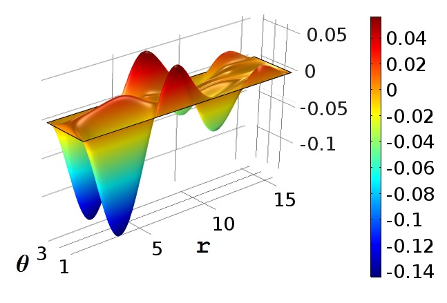
(a)  

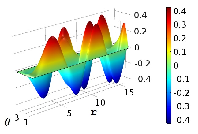
(b)  

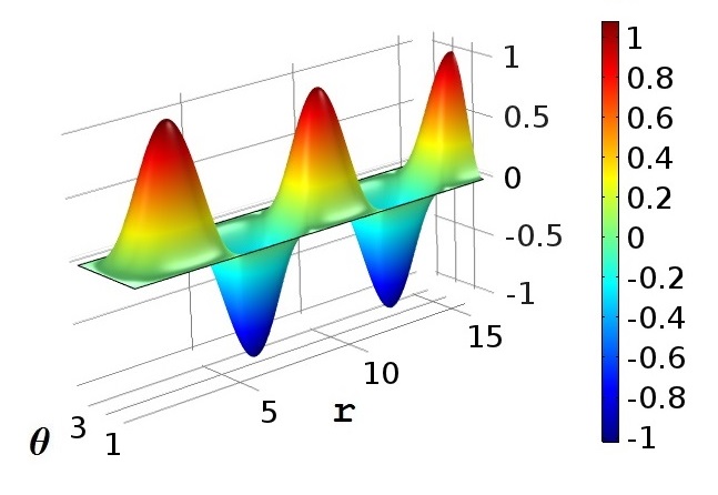
(c)  

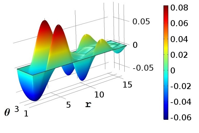
(d)  

Figure 1: Solution profile functions in the leading order: (a) ${\tilde{K}}_{1}^{(1)}$; (b) ${\tilde{K}}_{2}^{(1)}$; (c) ${\tilde{K}}_{4}^{(1)}$; (d) ${\tilde{K}}_{5}^{(1)}$ ($g=1,M=1$).

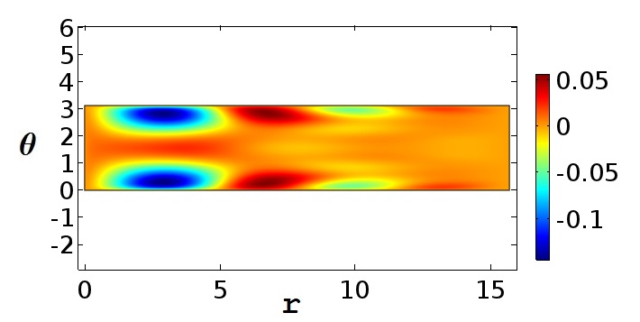
(a)  

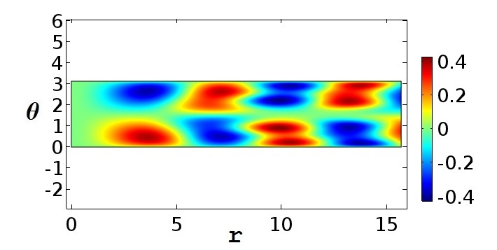
(b)  

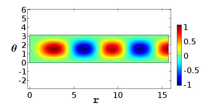
(c)  

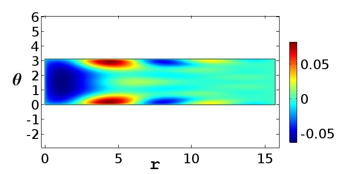
(d)  

Figure 2: Contour plots for the solution profile functions: (a) ${\tilde{K}}_{1}^{(1)}$; (b) ${\tilde{K}}_{2}^{(1)}$; (c) ${\tilde{K}}_{4}^{(1)}$; (d) ${\tilde{K}}_{5}^{(1)}$.

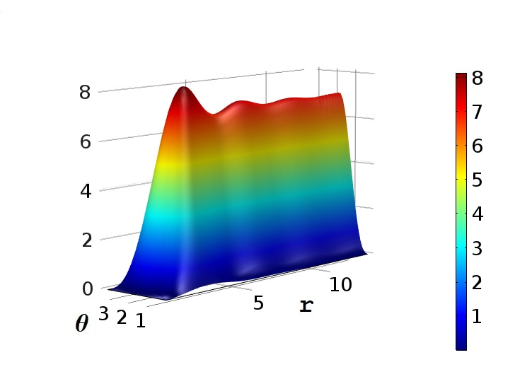
(a)  

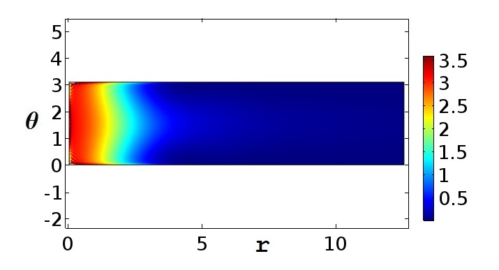
(b)  

Figure 3: (a) An integral energy density $r^{2}\sin\theta{\cal E}$ (averaged over the time period); (b) a contour plot for the time averaged energy density ${\cal E}$ ($g=1,M=1$).

The energy density is decreasing along the radial direction as $\dfrac{1}{r}$, and it has a maximum at the origin, and the total energy grows up linearly with increasing the radial size of a chosen numeric domain. Integration over the numeric domain constrained by $L=4\pi$ produces a value of the total energy $E_{II}^{tot}=121.6$ (up to multiplier factor $2\pi$ due to further integration over the azimuthal angle $\varphi$). Our numeric analysis of the solutions implies that solutions are determined by two parameters: the conformal parameter $M$ and the asymptotic amplitude $A_{0}$ of the Abelian field component mode $K_{4}(r,\theta,t)$. We fix the values of $M$ and $A_{0}$ to one, the amplitudes for other fields $K_{1,2,5}$ are obtained from the numeric solution. This allows to compare solutions with fixed values of $M,A_{0}$ and with different parities by evaluating their energies. The energy density of the stationary monopole-antimonopole pair solution with an opposite parity proposed in plb2017 has nearly the same shape and a total energy $E_{I}^{tot}=121.9$ which is very close to the value of $E_{II}^{tot}$. Note that a dominant contribution to the energy is provided by the field mode $K_{4}(r,\theta,t)$, it is $E(K_{4})=117.67$ (in units $g=1,M=1$). One should stress that our solution is completely different from known non-linear standing wave type solutions which have singularities.

2 Abelian regular stationary axially-symmetric solutions

Solutions determined by the boundary conditions (15) correspond to regular single-valued functions. Since the fields $K_{i}(r,\theta,t)$ represent components of the gauge potential which are not physical observables (unless the color symmetry is broken), one can choose boundary conditions with multi-valued intial profile functions as well. The gauge invariant quantities (like the energy, action etc) must be regular everywhere. In the leading order approximation one can find a local solution to the equations (13) near the origin $r=0$ in terms of the Taylor series expansion

$${\tilde{K}}_{1}^{(1)}=c_{1}(\dfrac{\pi}{2}-\theta)+\dfrac{1}{2}r^{2}(-c_{1}(\dfrac{\pi}{2}-\theta)+c_{5}\cos\theta)+O(r^{3}),$$

$${\tilde{K}}_{2}^{(1)}=-c_{1}r+O(r^{3}),$$

$${\tilde{K}}_{4}^{(1)}=c_{4}r^{2}\sin^{2}\theta+O(r^{3}),$$

$${\tilde{K}}_{5}^{(1)}=-c_{1}r(\dfrac{\pi}{2}-\theta)+c_{5}\cos\theta)+O(r^{3}),$$ (18)

where $c_{1,4,5}$ are arbitrary integration constants. One can verify that the local solution provides a regular energy density near the origin We impose periodic boundary conditions along the boundaries $(\theta=0,\pi)$ and the same asymptotic conditions (16). Wth this one can solve the system of equations (13), the obtained solution is presented in Fig. 4.

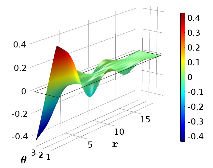
(a)  

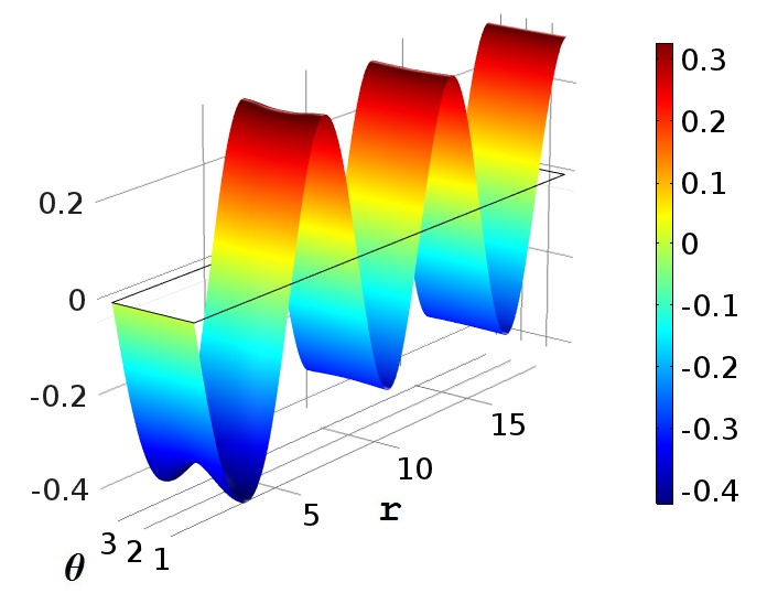
(b)  

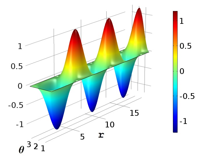
(c)  

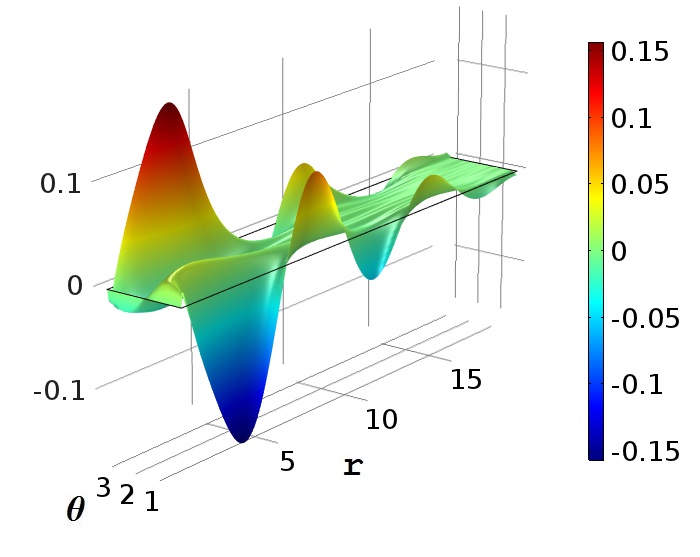
(d)  

Figure 4: Solution in the leading order: (a) $K_{1}^{(1)}$; (b) $K_{2}^{(1)}$; (c) $K_{4}^{(1)}$; (d) $K_{5}^{(1)}$.

The solution implies that azimuthal field strength components represent multi-valued functions along the $Z$-axis. However, a corresponding energy density is regular everywhere, and it has a similar shape as one in Fig. 3. A class of such solutions is determined by values of three parameters characterizing the asymptotic behavior, namely, by the conformal parameter $M$ and asymptotic amplitudes $a_{04},a_{02}$ of the oscillating modes $K_{2,4}$. Contrary to the case of type II solution, Fig. 1-3, the asymptotic amplitude $a_{02}$ of the mode ${\tilde{K}}_{2}^{(1)}$ is an additional free number parameter. In the limit $a_{02}\rightarrow 0$ the modes ${\tilde{K}}_{1,2,5}^{(1)}$ vanish identically, and one results in a solution which satisfies an Abelian type partial differential equation

$$\partial_{t}^{2}K_{4}-\partial_{r}^{2}K_{4}-\dfrac{1}{r^{2}}\partial_{\theta}^{2}K_{4}+\dfrac{\cot\theta}{r^{2}}\partial_{\theta}K_{4}=0.$$ (19)

In the case of $SU(2)$ Yang-Mills theory the equation (19) represents an equation of motion for one non-vanishing gauge field component $A_{\varphi}^{3}$. So, the Eq. (19) coincides identically with the equation of motion for one non-zero vector potential $A_{\varphi}$ of the Maxwell theory.

Let us consider in a detail the Abelian type solutions to Eq. (19). It is clear that solutions to this equation defines a corresponding class of non-Abelian solutions to the full set of $SU(2)$ or $SU(3)$ equations of motion within the reduction ansatz (2,4). A basis in the vector space of regular solutions to Eq. (19) is formed by the following functions:

$$K_{4}^{(k)}(r,\theta,t) = R_{k}(r)T_{k}(\theta)\sin(t),$$

$$R_{k}(r) = \sqrt{r}J_{\frac{2k+1}{2}}(r),$$

$$T_{k}(\theta) = \left\{\begin{array}[]{lcll}_{2}F^{1}[-\dfrac{k+1}{2},\dfrac{k}{2};\dfrac{1}{2};\cos^{2}\theta],&\rm{for~{}odd~{}}k,&\\ \cos\theta~{}_{2}F^{1}[-\dfrac{k}{2},\dfrac{k+1}{2};\dfrac{3}{2};\cos^{2}\theta],&\rm{for~{}even~{}}k,&\end{array}\right.$$ (22)

where $J_{n}(r)$ is the Bessel function of the first kind, ${}_{2}F_{1}(a,b;c;z)$ is the hypergeometric function, $k=1,2,3,...$, and integration constants $C_{1,2}$ are chosen in such a way to provide regular field configurations. One can write down first three basis solutions corresponding to values $k=1,2,3$

$$K_{4}^{(1)}(r,\theta,t) = (-\cos r+\dfrac{1}{r}\sin r)\sin^{2}\theta\sin t,$$

$$K_{4}^{(2)}(r,\theta,t) = \dfrac{1}{r^{2}}\big{(}3r\cos r+(-3+r^{2})\sin r\big{)}\cos\theta\sin^{2}\theta\sin t,$$

$$K_{4}^{(3)}(r,\theta,t) = \dfrac{1}{r^{3}}\big{(}r(r^{2}-15)\cos r+3(5-2r^{2})\sin r\big{)}\big{(}3+5\cos(2\theta)\big{)}\sin^{2}\theta\sin t.$$ (23)

The lowest mode $K_{4}^{(1)}(r,\theta,t)$ provides an interpolating function with a high accuracy for the numeric solution presented in the previous subsection, Fig. 1c. One can calculate the contribution of that mode to the total energy density in the numeric domain restricted by the parameter value $L=4\pi$. The total energy has a value $E(K_{4}^{(1)})=117.685$ which is very close to the value $E(K_{4})=117.67$ obtained from the numeric solution. The difference between two functions is 1.08 % by norm. Note that one has conformal classes of regular sttaionary solutions generated by the scaling transformation $r\rightarrow Mr,t\rightarrow Mt$ of the solutions (23).

III Weyl symmetric structure of the reduced Lagrangian

Let us consider first a simple case of a pure $SU(2)$ QCD. The corresponding Lagrangian can be written in explicit Weyl symmetric form using complex notations for the off-diagonal components of the gauge potential

$${\cal L} = -\dfrac{1}{4}F_{\mu\nu}^{2}-\dfrac{1}{2}|{D}_{\mu}{W}_{\nu}-{D}_{\nu}{W}_{\mu}|^{2}+igF_{\mu\nu}\stackrel{{\scriptstyle\ast}}{{W}}_{\mu}W_{\nu}-\dfrac{g^{2}}{2}\Big{[}(\stackrel{{\scriptstyle\ast}}{{W}}_{\mu}W_{\mu})^{2}-(\stackrel{{\scriptstyle\ast}}{{W}}_{\mu})^{2}(W_{\nu})^{2}\Big{]},$$ (24)

where

$$W_{\mu\nu}=-ig(\stackrel{{\scriptstyle\ast}}{{W}}_{\mu}W_{\nu}-\stackrel{{\scriptstyle\ast}}{{W}}_{\nu}W_{\mu}),$$

$${D}_{\mu}{W}_{\nu}=(\partial_{\mu}+igA^{3}_{\mu})W_{\nu},$$

$$W_{\mu}=\dfrac{1}{\sqrt{2}}(A^{1}_{\mu}+iA_{\mu}^{2}).$$ (25)

The Weyl symmetry is represented by the reflection transformation of the Abelian potential, $A_{\mu}^{3}\rightarrow-A_{\mu}^{3}$. A generalized DHN ansatz reads

$$A_{1}^{2} = K_{1},~{}~{}A_{2}^{2}=K_{2},~{}~{}A_{3}^{3}=K_{3},~{}~{}~{}A_{3}^{1}=K_{4},~{}~{}A_{4}^{2}=K_{5}.$$ (26)

After substitution of this ansatz into the Lagrangian one has cubic interaction terms

$${\cal L}_{cubic}=\dfrac{1}{r^{2}\sin^{2}\theta}\Big{[}K_{1}(K_{4}\partial_{r}K_{3}-K_{3}\partial_{r}K_{4})+K_{2}(K_{4}\partial_{\theta}K_{3}-K_{3}\partial_{\theta}K_{4})+K_{5}(-K_{4}\partial_{t}K_{3}-K_{3}\partial_{t}K_{4})\Big{]}.$$ (27)

The presence of the cubic interaction terms leads to breaking of the Weyl symmetry. As a consequence, the stationary monopole pair solution in a pure $SU(2)$ QCD does not possess Weyl symmetry. However, since the field component $K_{4}$ is suppressed in the leading order approximation, the Weyl symmetry of the Lagrangian takes place approximately.

Let us consider the case of the $SU(3)$ QCD. The Lagrangian can be written in complex notations as follows

$${\cal L}_{0} = \sum_{p=1,2,3}\Big{\{}-\dfrac{1}{6}(F_{\mu\nu}^{p})^{2}-\dfrac{1}{2}|D^{p}_{\mu}W_{\nu}^{p}-D_{\nu}^{p}W_{\mu}^{p}|^{2}-igF_{\mu\nu}^{p}W_{\mu}^{*p}W_{\nu}^{p}\Big{\}}+{\cal L}_{int}^{(4)}[W],$$

$$F_{\mu\nu}^{p} = \partial_{\mu}B_{\nu}^{p}-\partial_{\nu}B_{\mu}^{p},~{}~{}~{}~{}~{}~{}D^{p}_{\mu}W_{\nu}^{p}=(\partial_{\mu}-igB_{\mu}^{p})W_{\nu}^{p},~{}~{}~{}~{}~{}~{}B_{\mu}^{p}=A_{\mu}^{\alpha}{\vec{r}}_{\alpha}^{\,p},$$

$$W^{1}_{\mu} = \dfrac{1}{\sqrt{2}}(A_{\mu}^{1}+iA_{\mu}^{2}),~{}~{}~{}~{}~{}W^{2}_{\mu}=\dfrac{1}{\sqrt{2}}(A_{\mu}^{6}+iA_{\mu}^{7}),~{}~{}~{}~{}~{}W^{3}_{\mu}=\dfrac{1}{\sqrt{2}}(A_{\mu}^{4}-iA_{\mu}^{5}),$$ (28)

where the index $(p=1,2,3)$ corresponds to linear combinations of the gauge potentials which form the representation of the Weyl permutation group, and ${\vec{r}}_{\alpha}^{p}$ are the root vectors of the Lie algebra of $SU(3)$, the index $\alpha$ takes two values, ($\alpha=3,8$), corresponding to the generators of the Cartan algebra of $SU(3)$

$${\vec{r}}_{\alpha}^{\,1}=(1,0),~{}~{}~{}~{}{\vec{r}}_{\alpha}^{\,2}=(-1/2,\sqrt{3}/2),~{}~{}~{}~{}{\vec{r}}_{\alpha}^{\,3}=(-1/2,-\sqrt{3}/2).$$ (29)

First of all, note that the Lagrangian of a pure $SU(3)$ QCD in the form (28) can not be written in the Weyl symmetric form since the interaction term ${\cal L}_{int}^{(4)}$ is not factorized into a direct sum of parts corresponding to separated Weyl sectors. It is remarkable that applying the ansatz (4) one obtains an explicit Weyl symmetric reduced Lagrangian ${\cal L}_{red}(K_{1,2,4,5})$. In particular, the quartic interaction term originating from the kinetic part in (28) coincides identically with the Weyl symmetric expression for ${\cal L}_{int}^{(4)}$

$${\cal L}_{int}^{(4)}[W]=-\dfrac{9}{8}\sum_{p=1,2,3}\Big{[}(W^{*p\mu}W^{p}_{\mu})^{2}-(W^{*p\mu}W^{*p}_{\mu})(W^{p\nu}W^{p}_{\nu})\Big{]}.$$ (30)

Another essential feature of the reduced Lagrangian ${\cal L}_{red}(K)$ is that all cubic interaction terms are mutually canceled, in particular, the third term in (28) vanishes identically itself. As it is known, such a term represents an anomalous magnetic moment interaction which is responsible for the instability of the Savvidy vacuum savv ; N-O . Vanishing of this term gives an additional indication that stationary monopole-like solution could be stable under the gluon vacuum fluctuations. Indeed, it has been proved recently, that the vacuum made of stationary monopole-antimonopole pair is stable plb2017 . With this, the final expression for the reduced Lagrangian takes the following form

$${\cal L}_{red} = \sum_{p=1,2,3}\Big{\{}-\dfrac{1}{6}(F_{\mu\nu}^{p})^{2}-\dfrac{1}{2}|\partial_{\mu}W_{\nu}^{p}-\partial_{\nu}^{p}W_{\mu}^{p}|^{2}-\dfrac{9}{4}\sum_{p=1,2,3}\Big{[}(W^{*p\mu}W^{p}_{\mu})^{2}-(W^{*p\mu}W^{*p}_{\mu})(W^{p\nu}W^{p}_{\nu})\Big{]}.$$ (31)

The Lagrangian can be written in terms of four real independent fields $K_{i}(r,\theta,t)$

$${\cal L}_{red}(K) = \dfrac{3}{2r^{2}}\Big{[}r^{2}(\partial_{t}K_{1}-\partial_{r}K_{5})^{2}-\partial_{\theta}K_{1}^{2}+\partial_{\theta}K_{5}^{2}\Big{]}+\dfrac{3}{2r^{2}}\Big{[}\partial_{t}K_{2}(\partial_{t}K_{2}-2\partial_{\theta}K_{5})-\partial_{r}K_{2}(\partial_{r}K_{2}-2\partial_{\theta}K_{1})\Big{]}$$ (32)

$$+ \dfrac{9}{4r^{4}\sin^{2}\theta}\Big{[}r^{2}(\partial_{t}K_{4}^{2}-\partial_{r}K_{4}^{2})+\partial_{\theta}K_{4}^{2}\Big{]}-\dfrac{27}{4r^{4}\sin^{2}\theta}\Big{[}K_{4}^{2}(K_{2}^{2}+r^{2}(K_{1}^{2}-K_{5}^{2})\Big{]}.$$

One can observe immediately that the Lagrangian ${\cal L}_{red}(K)$ belongs to a field model with a simple quartic potential without derivatives. So that, on the space of special stationary solutions one has embedding of $\phi^{4}$ type model into the Yang-Mills theory.

IV Quantum stability

For simplicity we consider the quantum stability of the stationary wave type solution $K_{4}^{(1)}(r,\theta,t)$, (23), under small quantum gluon fluctuations in the case of a pure $SU(2)$ QCD. A general $SU(2)$ gauge potential $A_{\mu}^{a}$ is split into a sum of a classical background field $B_{\mu}^{a}$ and fluctuating quantum part $Q_{\mu}^{a}$. The background field represents the stationary solution

$$B_{\mu}^{a}=\delta_{\mu 3}\delta^{a,3}K_{4}^{(1)}(r,\theta,t).$$ (33)

The “Schrödinger” type equation for possible unstable quantum modes is the following plb2017

$$\mathscr{K}_{\mu}^{ab}\Psi_{\nu}^{b}=\lambda\Psi_{\mu}^{a},$$ (34)

where the operator $\mathscr{K}_{\mu}^{ab}$ corresponds to one-loop gluon contribution to the effective action plb2017

$$\mathscr{K}_{\mu\nu}^{ab} = -\delta^{ab}\delta_{\mu\nu}\partial^{2}_{t}-\delta_{\mu\nu}({\mathscr{D}}_{\rho}{\mathscr{D}}^{\rho})^{ab}-2f^{acb}{\mathscr{F}}_{\mu\nu}^{c},\quad$$ (35)

where the covariant derivative $\mathscr{D}_{\mu}$ and field strength $\mathscr{F}_{\mu\nu}$ are defined in terms of the classical background solution. The existence of solutions to Eq. (34) with negative eigenvalues $\lambda$ would indicate to the presence of unstable modes which destabilize the classical solution.

We choose a temporal gauge for the quantum gauge potential, this simplifies the matrix part of the operator $K_{\mu\nu}^{ab}$ and reduces the number of equations to nine elliptic second order partial differential equations on the three-dimensional domain $(0\leq r\leq L,0\leq\theta\leq\pi,0\leq t\leq\dfrac{2\pi}{M})$. Direct substitution of the classical solution

$$K_{4}^{(1)}(r,\theta,t) = A_{0}(-\cos(Mr)+\dfrac{1}{Mr}\sin(Mr))\sin^{2}\theta\sin(Mt)\equiv f_{0}(r,\theta,t),$$ (36)

into the eigenvalue equation (34) leads to factorization of the initial nine equations to three independent sets of equations which include the following functions: (I) $\Psi_{1}^{1},\Psi_{2}^{1},\Psi_{3}^{2}$, (II) $\Psi_{1}^{2},\Psi_{2}^{2},\Psi_{3}^{1}$, (III) $\Psi_{m}^{3}$ (m=1,2,3). The last group of equations corresponding to the Abelian direction in the color space represents free equations and do not produce negative modes. The second set of equations becomes identical to the first set of equations after changing variables $\Psi_{1}^{2}\rightarrow\Psi_{1}^{1},\Psi_{2}^{2}\rightarrow\Psi_{2}^{1},\Psi_{3}^{1}\rightarrow\Psi_{3}^{2}$ and reflection of the background field, $f_{0}\rightarrow-f_{0}$. So one has to solve only one system of three eigenvalue equations

$$-\Delta\Psi_{1}^{1}+\dfrac{1}{r^{2}}\Big{(}(2+\csc^{2}\theta f_{0}^{2})\Psi_{1}^{1}+2(\cot\theta+\partial_{\theta})\Psi_{2}^{1}-2\csc\theta(f_{0}-r\partial_{r}f_{0})\Psi_{3}^{2}\Big{)}=\lambda\Psi_{1}^{1},$$

$$-\Delta\Psi_{2}^{1}+\dfrac{1}{r^{2}}\Big{(}\csc^{2}\theta(1+f_{0}^{2})\Psi_{2}^{2}-2\partial_{\theta}\Psi_{1}^{1}-2\csc\theta(\cot\theta f_{0}-\partial_{\theta}f_{0})\Psi_{3}^{2}\Big{)}=\lambda\Psi_{2}^{1},$$

$$-\Delta\Psi_{3}^{2}+\dfrac{1}{r^{2}}\Big{(}(1+\cot^{2}\theta+\csc^{2}\theta f_{0}^{2})\Psi_{3}^{2}-2\csc\theta(f_{0}-r\partial_{r}f_{0})\Psi_{1}^{1}-2\csc\theta(\cot\theta f_{0}-\partial_{\theta}f_{0})\Psi_{2}^{1}\Big{)}=\lambda\Psi_{3}^{2},$$

$$\Delta\equiv\partial^{2}_{t}+\partial^{2}_{r}+\dfrac{2}{r}\partial_{r}+\dfrac{1}{r^{2}}\partial^{2}_{\theta}+\dfrac{\cot\theta}{r^{2}}\partial_{\theta},$$ (37)

where $\Delta$ is a part of the vector Laplace operator. The system of equations (37) corresponds to a quantum mechanical potential problem of three interacting particles. The equations contain positive centrifugal potentials depending on space coordinates $(r,\theta)$ and two different attractive potentials

$$V_{1} = -\dfrac{2\csc\theta}{r^{2}}(f_{0}-r\partial_{r}f_{0}),$$

$$V_{2} = -\dfrac{2\csc\theta}{r^{2}}(\cot\theta f_{0}-\partial_{\theta}f_{0}).$$ (38)

One can verify that potentials $V_{1}$ and $V_{2}$ have no dangerous singularities at the origin $r=0$, they are finite everywhere and decrease along the radial direction as $\dfrac{1}{r}$ and $\dfrac{1}{r^{2}}$ respectively. It is clear, that such potentials lead to a positive eigenvalue spectrum at small enough values of the parameters $A_{0},M$. Exact numeric solving the system of equations confirms absence of negative modes, Fig. 5.

(a)  

(b)  

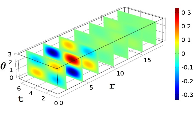
(c)  

Figure 5: Eigenfunctions corresponding to the lowest eigenvalue $\lambda=0.0298$: (a) $\Psi_{1}^{1}$; (b) $\Psi_{2}^{1}$; (c) $\Psi_{3}^{2}$.

In conclusion, we propose a new class of regular stationary solutions with a finite energy density in a pure $SU(3)$ QCD. Recently it has been proved that the stationary spherically symmetric monopole and monopole-antimonopole pair solutions are stable against small quantum gluon fluctuations plb2017 ; prd2017 . We expect that the whole class of considered regular stationary solutions possesses quantum stability as well. We have considered a class of regular Abelian stationary solutions and have proved thier stability under small quantum gluon fluctuations. Since the Abelian solutions possess the classical stability as well, they provide the most preferable field configurations for the QCD vacuum in quasiclassical approximation. We suppose that the regular stationary solutions play an important role in microscopic description of the QCD vacuum formation. This issue will be considered in the forthcoming paper.

References

• (1) Y. Nambu, Phys. Rev. D10, 4262 (1974).
• (2) S. Mandelstam, Phys. Rep. 23C, 245 (1976).
• (3) A. Polyakov, Nucl. Phys. B120, 429 (1977).
• (4) G. ’t Hooft, Nucl. Phys. B190, 455 (1981).
• (5) G.K. Savvidy, Phys. Lett. B71, 133 (1977).
• (6) N.K. Nielsen and P. Olesen, Nucl. Phys. B144, 376 (1978).
• (7) H.B. Nielsen and M. Ninomiya, Nucl. Phys. B156, 1 (1979).
• (8) H.B. Nielsen and P. Olesen, Nucl. Phys. B160, 380 (1979).
• (9) J. AmbjΓΈrn and P. Olesen, Nucl. Phys. B170, 60 (1980).
• (10) J. AmbjΓΈrn and P. Olesen, Nucl. Phys. B170, 265 (1980).
• (11) M. Chernodub, Phys. Lett. B730, 63 (2014).
• (12) M. Engelhardt, K. Langfeld, H. Reinhardt, O. Tennert, Phys. Rev. D61, 054504 (2000).
• (13) J. Greensite, Confinement from Center Vortices: A review of old and new results, arXiv: 1610.06221 (2016).
• (14) P. Olesen, A center vortex representaton of the classical SU(2) vacuum, arXiv: 1605.00603 (2016).
• (15) Y. M. Cho, Nucl. Phys., A844 (2010) 120C-137C.
• (16) Y. M. Cho, Int. J. Mod. Phys. 29 (2014) 1450013.
• (17) M. Chernodub, Phys. Rev. Lett., 95252002 (2005).
• (18) D. Diakonov, V. petrov, AIP Conf. Proc. 1343 (2011) 69-74.
• (19) B.-H. Lee, Y. kim, D.G. Pak, T. Tsukioka, P.M. Zhang, Int. J. Mod. Phys., A32 (2017)1750062.
• (20) D.G. Pak, B.-H.- Lee, Y. Kim, T. Tsukioka, P.M. Zhang, On microscopic structure of the QCD vacuum , arxiv: 1703.09635 (2017).
• (21) R. Dashen, B. Hasslacher and A. Neveu, Phys. Rev. D10 (1974) 4138.
• (22) C.Rebbi and P. Rossi, Phys. Rev. D 22, 2010 (1980).
• (23) J. Kunz, B. Kleihaus and Y. Brihaye, Phys. Rev. D 46, 3587 (1992).
• (24) G.K. Savvidy, Phys. Lett. B71, 133 (1977).
• (25) N.K. Nielsen and P. Olesen, Nucl. Phys. B144, 376 (1978).
• (26) Y. Kim, B.-H. Lee, D.G. Pak, Ch. Park, T. Tsukioka, Phys. Rev. D 96, 054025 (2017).