A Fast Radio Burst Search Method for VLBI Observation

Abstract

We introduce the cross spectrum based FRB (Fast Radio Burst) search method for VLBI observation. This method optimizes the fringe fitting scheme in geodetic VLBI data post processing, which fully utilizes the cross spectrum fringe phase information and therefore maximizes the power of single pulse signals. Working with cross spectrum greatly reduces the effect of radio frequency interference (RFI) compared with using auto spectrum. Single pulse detection confidence increases by cross identifying detections from multiple baselines. By combining the power of multiple baselines, we may improve the detection sensitivity. Our method is similar to that of coherent beam forming, but without the computational expense to form a great number of beams to cover the whole field of view of our telescopes. The data processing pipeline designed for this method is easy to implement and parallelize, which can be deployed in various kinds of VLBI observations. In particular, we point out that VGOS observations are very suitable for FRB search.

1 Introduction

Fast radio bursts (FRBs) are high flux radio flashes with milliseconds duration. At present the burst mechanism is still not clear (Thornton et al., 2013; Keane et al., 2016; Chatterjee et al., 2017). The high dispersion measure (DM) of current detections suggest their extragalactic origin . However, the possibility of Galactic origin still cannot be excluded, because the extra DM may be intrinsic to the source (Katz, 2016a).

FRB was first discovered in 2007 when reanalyzing the archive data of Parkes radio telescope (Lorimer et al., 2007). Until now, about 20 FRBs are detected with large single dish telescopes and the UTMOST (Caleb et al., 2016) interferometer. The angular resolution of these instruments is still not sufficient to unambiguously associate the burst with the background counterpart. Among those events, most of them are non-repeating burst. The only repeating burst FRB 121102 (Spitler et al., 2016; Scholz et al., 2016) provides a good chance to obtain its high precision location via VLBI observation. Chatterjee et al. (2017) reveal that FRB 121102 originates within 100 mas of a faint 180 mJy persistent and compact radio source which is associate with an optical counterpart. Marcote et al. (2017) show for the first time that the bursts and the source are co-located with an angular separation of less than 12 mas (a projected linear separation of less than 40 pc) by using the EVN (European VLBI Network) data. Tendulkar et al. (2017) classify the counterpart as a low-metallicity, star forming dwarf galaxy at a redshift of $z$ = 0.19273(8). Bassa et al. (2017) find the burst is coincident with a star forming region of the host galaxy. Scholz et al. (2017) carry out observations of the burst simultaneously in X-ray, Gamma-ray and radio band.

Until now, it is still not clear if non-repeating and repeating bursts have the same origin. Catastrophic event models are able to explain non-repeating burst (Dai et al., 2016), including the merger of compact objects (Kashiyama et al., 2013; Wang et al., 2016), super massive neutron stars collapsing to black holes (Falcke & Rezzolla, 2014; Zhang, 2014), and so on. The repeating burst is more likely to originate from young remnants of stellar collapses, neutron stars or black holes (Katz, 2016a), e.g. soft gamma repeaters (Pen & Connor, 2015; Katz, 2016c), giant pulse from young pulsars (Keane et al., 2012; Katz, 2016b), and the interaction of pulsars with planets (Mottez & Zarka, 2014), asteroids or comets (Geng & Huang, 2015; Dai et al., 2016).

Nowadays FRB search is a hot topic in radio astronomy. The high precision localization of the burst is the key to identify background counterpart and finally explain the burst mechanism (Masui et al., 2015) . Since the angular resolution of single dish telescope is low, it is very necessary to develop interferometer based method to achieve a higher resolution. UTMOST (Caleb et al., 2016) is the first radio interferometer search at 843 MHz for fast transits, particularly FRB. Until 2017, 3 FRBs have been discovered in a 180-day survey of the Southern sky (Caleb et al., 2017). However, its angular resolution (15 sec $\times$ 8.4 degree) is still not enough to identify background counterparts unambiguously. In this condition, VLBI (Very Long Baseline Interferometer, Whitney et al., 1976; Rogers et al., 1983; Thompson et al., 2001) search with even higher angular resolution is very necessary.

There have been efforts to search for FRB signals in regular VLBI observations. The V-FASTR project (Wayth et al., 2011; Thompson et al., 2011) ran commensally on VLBA and aimed at providing a few tens of milliarcsecond localization of detected FRB. Until 2016, the project had not detected any FRB, but it helped setting the upper limit of FRB event rate (Burke-Spolaor et al., 2016). The LOCATe project (Paragi, 2016) aimed at establishing an FRB pipeline for the EVN (European VLBI Network). The project was based on the well-developed calibration pipeline and the EVN software correlator SFXC (Keimpema et al., 2015). In the test phase, the pipeline had successfully detected single pulses from test source RRAT J1819-1458 (McLaughlin et al., 2007), and localized the pulse position in image plane. In general, the pipeline of V-FASTR and LOCATe are similar. We summarize them as the auto spectrum based method: They take the auto spectrum from the correlator, carry out RFI excising and dedispersion. After that standard pulsar search tools, e.g. PRESTO (Ransom, 2001) are used to detect single pulses. When a single pulse is identified in multiple stations, raw data at that time range are re-correlated, calibrated and finally used for localization.

VLBI technology has been widely used in the field of astrophysics (Fish et al., 2016), geodesy and astrometry (Ma et al., 1998, 2009; Schuh & Behrend, 2012; Behrend, 2013; Altamimi et al., 2016), deep space exploration (Duev et al., 2012). For geodetic VLBI, observations are scheduled in high frequency (e.g., once per week), and usually involve tens of stations for one session. Since large volume storages are very expensive, in standard data processing procedure, the large amount of VLBI raw observation data are deleted immediately after correlation. In authors’ view, these data are not only important for geodetic purpose, but also valuable for various kinds of time domain astronomy studies. It is such a good chance to carry out FRB search that the deletion of raw data is a huge loss. However, when developing our own FRB search pipeline for these data, we realize that the electromagnetic environment of some geodetic VLBI stations are not ideal. According to our study, the popular auto spectrum based method might not always behave well in single pulses extraction from RFI contaminated data. To fully exploit these data, we have to develop new method.

In this work, we introduce the cross spectrum based single pulse search method. This method takes the idea of geodetic VLBI data processing and fully utilizes the fringe phase information of cross spectrum. By carrying out fringe fitting on each cross spectrum of milliseconds duration, the power of single pulse signal is maximized. In this way single pulses are extracted from given time range and baseline. Our method is good at extracting single pulses from RFI contaminated data, which is very suitable for FRB search in various kinds of VLBI observations.

This paper is organized as follows. In Sec. 2, we introduce the cross spectrum based FRB search method, including the fringe fitting scheme, dedispersion and time segment construction, single pulse detection strategy, etc. In Sec. 3, we carry out single pulse search in a data set of VLBI pulsar observation and validate the search result with predicted pulsar phase. In Sec. 4, we investigate the possibility of FRB search in VGOS observation. In Sec. 5, we discuss issues not covered in previous sections. In Sec. 6, we summarize the whole work.

2 The cross spectrum based single pulse search method

In this section, we introduce the cross spectrum based single pulse search method: VLBI raw data from each station are first correlated and output as APs (Accumulation period, or integration period) of milliseconds duration. Then several APs are summed together along time axis to construct time segments with given window length. After that fringe fitting is carried out independently for these time segments of multiple window lengths. Finally single pulse are extracted from each baseline and cross matched on multiple baselines.

Besides above mentioned procedures, we have to point out that the search of dispersion measure is also an important part in the whole search procedure. We have proposed a whole set of DM search scheme and present it in Sec. 5.3. For the pulsar observation data used in this work, the DM value is too small, which is not suitable for the testing of the DM search scheme.

2.1 VLBI correlation

VLBI correlation is the fist step of the whole single pulse search procedure. In general, any FX type correlator that supports Mark5b (Whitney, 2003) or VDIF (Whitney et al., 2009) format raw data decoding and is able to generate visibility (cross spectrum) output with milliseconds duration is competent for the work. Before the correlation of target scans, the clock offset and rate must be well adjusted with the calibration source, such that the residual delay is limited to one sample period and the fringe rate (residual delay rate multiplied with sky frequency) is no larger than $10^{-2}$ Hz. Since VLBI correlation is a time consuming process, a correlator that is able to fully exploit the computation power of modern CPU/GPU cluster is preferred. This is especially important for real time data correlation.

2.2 Dedispersion and the construction of time segment

Let $S(n,j,k)$ represent the complex visibility of cross spectrum for a given baseline. Here $n,~{}j,~{}k$ correspond to the $n$-th sky frequency channel, the $j$-th frequency point inside the sky frequency channel and the $k$-th AP. Due to dispersion, the arrival time of a single pulse is a function of dispersion measure (DM) and frequency. With given DM and reference frequency $f_{\mathrm{ref,dm}}$, the time offset $\Delta t$ of $j$-th frequency point in $n$-th frequency channel with respect to $f_{\mathrm{ref,dm}}$ is (Lorimer & Kramer, 2004):

$$\Delta t=4.15\times 10^{6}\times\mathrm{DM}\times\left[\frac{1}{(f_{0}^{n}+f_{j})^{2}}-\frac{1}{f_{\mathrm{ref,dm}}^{2}}\right],$$ (1)

where $f_{0}^{n}$ is the sky frequency of $n$-th channel, $f_{j}$ is the baseband frequency of $j$-th frequency point, time and frequency take the unit of millisecond and MHz, respectively. In this work, $f_{\mathrm{ref,dm}}$ always takes the highest frequency of the band, such that $t_{\mathrm{offset}}$ is nonnegative. $\Delta t$ is further mapped to the offset of AP index $\Delta k$:

$$\Delta k=\lfloor 0.5+\Delta t/t_{\mathrm{ap}}\rfloor,$$ (2)

where $t_{\mathrm{ap}}$ is the duration of AP. The time segment is constructed by summing the cross spectrum within the window along the time axis:

$$S_{k_{0},l}(n,j)=\sum_{k=k_{0}+\Delta k}^{k_{0}+\Delta k+l-1}S(n,j,k),$$ (3)

where $S_{k_{0},l}$ represents the time segment starting with AP index $k_{0}$ and summing along the time axis with a window length $l$; $n$, $j$ represent the $n$-th sky frequency channel and the $j$-th frequency point inside the sky frequency channel. Time segment is the basic unit of this work. We will carry out fringe fitting independently for time segments of different window lengths. One may find that $\Delta k$ is a function of $n,j$, which means in a time segment each frequency point might have its own starting and ending AP index. In Sec. 2.3, we will explain the time segment constructed in this way can be used for fringe fitting as long as the corresponding fringe rate (delay rate times sky frequency) is small.

2.3 Fringe fitting

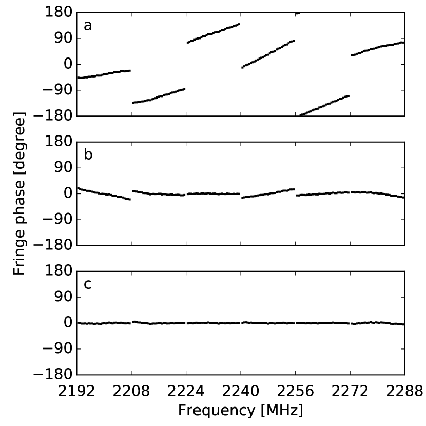
Figure 1: Demonstration of fringe fitting process. Panel a: Fringe phase before fringe fitting. Panel b: Fringe phase after fringe fitting, with initial phase calibration only. Panel c: Fringe phase after fringe fitting, with both initial phase and channel delay calibration. Data are taken from calibration source 3C273 of VLBI pulsar observation, Km-Ur baseline, 10 s duration. 6 stripes in each panel correspond to 6 frequency channels in S band. Each frequency channel contains 32 frequency points. The first point of each channel is not plotted in the figure, since it does not take part in fringe fitting as explained in Sec. 2.3.

Fringe fitting is a key step in geodetic VLBI data post processing. As demonstrated in Fig. 1, panel a, the fringe phase of visibility output is not flat before calibration, which leads to a low amplitude (power) of summed cross spectrum across the band. The purpose of fringe fitting is to find out residual delay, delay rate and initial phase across the band, and carry out fringe phase rotation accordingly (Cotton, 1995; Takahashi, 2000; Cappallo, 2014). After fringe fitting, the fringe phase across the whole band becomes flat and the amplitude of the summed cross spectrum is maximized. In this work, we take the algorithm of geodetic VLBI fringe fitting which is implemented in Haystack Observatory Postprocessing System (HOPS), and make some modifications for higher accuracy and better performance.

The delay resolution function is defined as the summed cross spectrum after phase rotation (Takahashi, 2000):

$$G(\Delta\tau_{\mathrm{s}},\Delta\tau_{\mathrm{m}},\Delta\dot{\tau})=\sum_{n=0}^{N-1}\sum_{j=1}^{J-1}\sum_{k=0}^{K-1}S(n,j,k)e^{-i\Phi(n,j,k)}$$

with

$$\Phi(n,j,k) = 2\pi f_{j}\Delta\tau_{\mathrm{s}}+2\pi(f_{0}^{n}-f_{\mathrm{ref,fit}})\Delta\tau_{\mathrm{m}}$$ (4)

$$+ 2\pi f_{0}^{n}\Delta\dot{\tau}t_{\mathrm{ap}}k+\Delta\phi_{0}^{n},$$

where $\Delta\tau_{\mathrm{s}},\Delta\tau_{\mathrm{m}},\Delta\dot{\tau}$ are the multi band residual delay (MBD), the single band residual delay (SBD) and the delay rate, respectively; $f_{\mathrm{ref,fit}}$ is the reference frequency for fringe fitting; $\Delta\phi_{0}^{n}$ is the initial phase of $n$-th frequency channel. The triple summations are made for $N$ frequency channels across the band, $J-1$ frequency points inside one frequency channel and $K$ APs. Note that the summation of frequency points excludes $j=0$, so as to eliminate the offset of the correlation function (Takahashi, 2000). The fringe fitting procedure finds out MBD, SBD and delay rate that maximize the delay resolution function.

In a regular VLBI correlation, the fringe rate ($f_{0}^{n}\Delta\dot{\tau}$) of the cross spectrum is well limited to $10^{-2}$ Hz. The corresponding phase change due to fringe rate is small in a short time range (e.g. hundred milliseconds). As a modification to the standard fringe fitting algorithm, in this work, the term $2\pi f_{0}^{n}\Delta\dot{\tau}t_{\mathrm{ap}}k$ is neglected in Eq. 4. A direct consequence is APs of milliseconds duration can be summed up directly with Eq. 3 to construct a time segment. Fringe fitting now becomes SBD and MBD search for each time segment, which reduces computation complexity.

Eq. 4 is based on the assumption that all frequency channels share the same SBD. However, in real situation, channel delays exist due to the non-ideal instrument, which lead to the different slopes of fringe phase in each frequency channel. Since we use only one SBD to fit all frequency channels, the resulting fringe phase across the band are not flat (Fig. 1, panel b). According to our study, this leads to the 5 - 10 percent loss of power compared with the ideally flat fringe phase. For geodetic VLBI that always observe strong sources with hundred seconds duration, current fringe fitting scheme is good enough to achieve the desired SNR (signal to noise ratio). However, in this work, we detect single pulse signals with milliseconds duration. This extra power is very important. To make fringe phase flat, one direct approach is to fit SBD for every individual frequency channel. Obviously this is time consuming. We take another approach, by making an extra phase rotation $-2\pi(f_{j}-f_{\mathrm{bw}}/2)\Delta\tau_{0}^{n}$ for every frequency point in a time segment before fringe fitting. Here $\Delta\tau_{0}^{n}$ comes from the calibration source, which is derived by fitting the channel delay of $n$-th frequency channel. After this phase rotation, all frequency channels of the time segment share the same SBD. The fringe phase across the band becomes much flatter after fringe fitting, which is shown in Fig. 1, panel c. Note that above treatment is based on an assumption that delay differences between channels are constant in the whole observation. According to our fit to the 24 hours geodetic VLBI observation session, this is roughly the case.

After above two modifications, Eq. 4 becomes:

$$G_{k_{0},~{}l}(\Delta\tau_{\mathrm{s}},\Delta\tau_{\mathrm{m}})=\sum_{n=0}^{N-1}\sum_{j=1}^{J-1}S_{k_{0},~{}l}(n,j)e^{-i\Phi(n,j)}$$

with

$$\Phi(n,j) = 2\pi f_{j}\Delta\tau_{\mathrm{s}}+2\pi(f_{0}^{n}-f_{\mathrm{ref,fit}})\Delta\tau_{\mathrm{m}}$$ (5)

$$+ 2\pi(f_{j}-f_{\mathrm{bw}}/2)\Delta\tau_{0}^{n}+\Delta\phi_{0}^{n},$$

where $G_{k_{0},~{}l}(\Delta\tau_{\mathrm{s}},\Delta\tau_{\mathrm{m}})$ represents the delay resolution function of time segment $S_{k_{0},~{}l}$. A relatively detailed explanation of channel delay $\Delta\tau_{0}^{n}$ and initial phase $\Delta\phi_{0}^{n}$ extraction is given in appendix A.

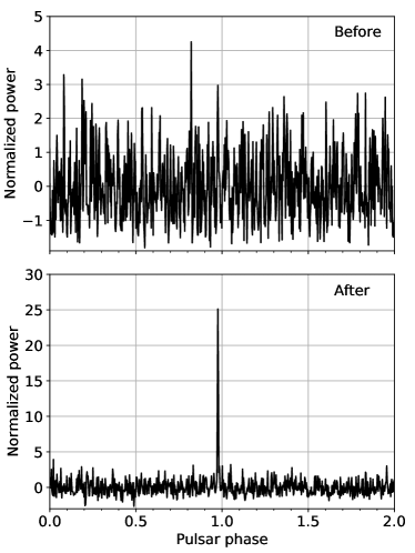
Figure 2: (a)

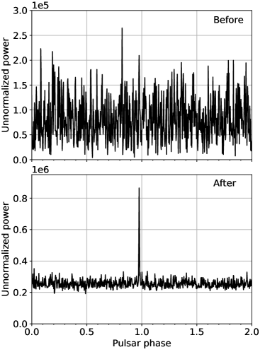
Figure 3: (b)

Figure 4: Signal power before and after fringe fitting. The pulsar phase and power of each time segment in the given time range is plotted. Panel a and b present the normalized and unnormalized (raw) power, respectively. The single pulse is detected at 49.1 s of scan 73, Sh-Ur baseline, and is shown as a cyan circle at corresponding time and scan in Fig. 7. The window length of time segments demonstrated in this figure is 4.096 ms. The phase of the single pulse is consistent with the pulsar phase range (0.973 - 0.983).

Panel a of Fig. 4 demonstrates the normalized power of each time segment before and after fringe fitting. It clearly shows that the normalized power of the single pulse around pulsar phase 0.978 is less than the threshold (we set it to 3 in Sec. 2.4) before fringe fitting, and is therefore not detectable. After fringe fitting, the power of the single pulse signal is greatly enhanced. The normalized power is defined as:

$$P_{\mathrm{norm}}=\left(|G|-|G|_{\mathrm{average}}\right)~{}/~{}|G|_{\sigma},$$ (6)

where $|G|$ is the amplitude of delay resolution function (summed power of cross spectrum) for each time segment, $|G|_{\mathrm{average}}$ is the average of $|G|$ in a given time range, $|G|_{\sigma}$ is the standard deviation of $|G|$. Note the calculation of normalized power are baseline based. Panel b of Fig. 4 demonstrates the unnormalized power. As shown in the bottom panel of Fig. 4.b, most of the time no single pulse signal is detected. The average power $|G|_{\mathrm{average}}$ corresponds to the system noise (Lorimer & Kramer, 2004), and can be estimated with correlation theory:

$$S_{\mathrm{noise}}=\sqrt{\frac{\mathrm{SEFD}_{1}\cdot\mathrm{SEFD}_{2}}{2BT}},$$ (7)

where $S_{\mathrm{noise}}$ is in unit of Jansky (Jy), $B$ is the observation bandwidth, $T$ is the integration time, which corresponds to the window length in this work. The deviation of Eq. 7 takes the definition of SNR in Takahashi (2000), and assumes the normal observation conditions that the antenna temperature of the radio source is much smaller than the system noise. Generally speaking, it is not required that the signal power is much larger than the average noise as demonstrated in Fig. 4. A single pulse is already detectable if its power is several times larger than the noise fluctuation $|G|_{\sigma}$. This is the reason the detection threshold is in unit of noise fluctuation in this work.

2.4 Single pulse extraction

We test two schemes of extracting single pulses from multiple baselines. In the first scheme, candidate signals are first detected and filtered on multiple windows, then they are cross matched on multiple baselines. In the second scheme, the power of multiple baselines are summed together to achieve a higher sensitivity, then single pulses are extracted via multiple windows filtering. Below we describe these two schemes in detail.

2.4.1 Multiple baselines cross matching scheme

•  Single pulse extraction from one baseline

Figure 5: Single pulse detected in multiple windows. The single pulse shown here is the same one as in Fig. 4. Error bars of different length correspond to the range of time segments with their respect window lengths. The gray region corresponds to the pulsar phase range (0.973 - 0.983).

For each baseline, we prepare several lists of time segments with different window lengths. The length of windows may range from one to ten times of a single pulse duration. By filtering signals with multiple windows, most RFI can be effectively excluded. Note that two consecutive time segments inside a list are half overlapped, e.g, the time segments are constructed as $S_{k_{0},l}$, $S_{k_{0}+l/2,l}$, $S_{k_{0}+l,l}$, etc. This is to prevent the possible detection failure when a single pulse locates at the border of two interconnect time segments.

After the construction of time segments, we carry out fringe fitting for each time segment and derive the normalized power with Eq. 6. In this work, we set a threshold of 3 for normalized power, signals with normalized power higher than 3 are kept for further filtering. For each window, a series of candidate signals are identified. Then the candidate signals are filtered with multiple windows to exclude RFI. The reason to use multiple windows is based on the assumption: a single pulse with FRB or pulsar origin should be detectable in more than one window, and its MBD values in these windows are similar. In contrast, RFIs with terrestrial origin would not be so stable and their MBD values are quite different in these windows. In general, the procedure of single pulse detection on one baseline is summarized below.

• Constructing time segments with multiple window lengths. Carrying out fringe fittings for these time segments. Selecting candidate signals. A selected candidate signal is uniquely described with time range, MBD and normalized power.

• Starting with the largest window, inserting candidate signals of each window to candidate groups. If the time range of a candidate signal is overlapped with any candidate signal that belongs to a candidate group, inserting it to that group; otherwise creating a new candidate group and inserting again.

• Calculating the average value of MBD $\bar{\Delta\tau_{\mathrm{m}}}$. Removing candidate signals with MBD outside the range ($\bar{\Delta\tau_{\mathrm{m}}}-t_{\mathrm{ambig}}/4,~{}\bar{\Delta\tau_{\mathrm{m}}}+t_{\mathrm{ambig}}/4$). Here $t_{\mathrm{ambig}}$ is the ambiguity of MBD (Takahashi, 2000) and must be take into account when calculating average and removing data.

• Calculating the number of different windows $N_{\mathrm{win}}$ in the candidate group. A single pulse is assumed to be found if it is detected in at least $N_{\mathrm{win,min}}$ windows in the group. The candidate signal with the highest power is assumed to be the best estimation of the single pulse, and is kept for multiple baselines cross matching in the next step. The corresponding power and width are regarded as the characteristic power and width of the single pulse.

Fig. 5 presents a single pulse detected on multiple windows. In some windows, several time segments catch the single pulse with different powers. It clearly shows that time segment of which the window length is comparable with the single pulse and the location is inside the pulsar phase range yields the highest power. Therefore, the cross spectrum method is able to estimate the width and location of the single pulse with the resolution of window length.

•  Cross matching of multiple baselines

After single pulses are detected on multiple baselines, they are inserted to the cross matching groups. If the time range of one single pulse is overlapped with any single pulse in a cross matching group, it is inserted to that group; otherwise a new cross matching group is created and the single pulse is inserted. After insertion, we calculate the number of different baselines in each cross matching group. Single pulses detected on 2 or more baselines can almost excluded the possibility of RFI.

2.4.2 Multiple baselines power summation scheme

In the test of single pulse detection from pulsar observation data, we find that the cross matching scheme is quite accurate in detecting pulsar signals. However, only a small number of pulsar signals are detected on low sensitivity baselines (e.g., Sh related baselines). The main reason is a significant amount of pulsar signals are so weak that they are not detectable if the baseline sensitivity is too low. To improve the detection sensitivity, in this scheme, we first combine the power of several baselines, then extract single pulses via multiple windows filtering. The detailed implementation is described below.

• Preparing time segments of multiple window lengths for each baseline and then carrying out fringe fitting for these time segments. This step is the same as step a of previous scheme.

• For each baseline, calculating the power (amplitude of delay resolution function) of each time segment after fringe fitting. Combining several baselines by summing the power of corresponding time segments together, then selecting candidate signals with given threshold. This is done for time segments of each window length.

• Filtering the single pulse with multiple windows, which is the same as step b in previous scheme. For the combined baseline, the MBD information is of no use. Therefore step c of previous scheme is skipped.

• Extracting single pulses from the candidate group, which is the same as step d in previous scheme.

According to our test, we indeed improve the detection sensitivity for a less sensitive station by combining baselines of that station.

3 Single pulse detection in VLBI pulsar observation

In this section, we exhibit our detection of single pulses from a data set of VLBI pulsar observation using the cross spectrum based method. Since the observed pulsar has been well studied, we could validate if a singe pulse originates from the pulsar or not via the predicted pulsar phase generated by TEMPO2 (Hobbs et al., 2006).

3.1 Observation overview

Table 1: Parameter setting of VLBI pulsar observation.

Parameter	Setting
Experiment code	psrf02
Observation date	Feb. 15, 2015 (MJD 57068)
Observation time	Start: UTC 08h00m00s
	Stop:  UTC 20h01m40s
Station	Sh, Km, Ur
Target source	PSR J0332+5434
Reference source	J0347+5557
Calibration source	J1044+719, 3C273
Frequency band	S, X
Data collector	CDAS (Zhu et al., 2016)
Polarization	Right circular
Frequency channel	6 in S band, 10 in X band
Bandwidth per channel	16 MHz
Sample bits	2

The VLBI data used in this work are taken from Chinese VLBI Network (CVN, Zheng, 2015) pulsar observation in 2015 (Chen et al., 2015). Three CVN antennas (Sh, Km, Ur) take part in the observation. Their performance are listed in Tab. 7. The main purpose of this observation is to obtain the accurate position of PSR J0332+5434 (B0329+54) using VLBI phase reference method (Thompson et al., 2001). PSR J0332+5434 is one of the brightest pulsars in the Northern sky. The average flux at S band is 0.1 Jy (Kramer et al., 2003). According to ATNF Pulsar Catalogue (Manchester et al., 2005), the pulsar has a dispersion measure of 26.833 $\mathrm{pc~{}cm}^{-3}$ and a period of 0.7145 s. Parameters of this observation are listed in Tab. 1.

Table 2: Performance of 3 CVN antennas.

Antenna	Diameter	SEFD
name	(m)	(Jy)
Sh	25	800
Km	40	350
Ur	25	560

In this work, we use 6 frequency channels in S band for single pulse search. The 96 MHz bandwidth in S band (2192 MHz - 2288MHz) is divided into 6 16 MHz interconnected frequency channels. Each frequency channel contains 32 frequency points. As explained in Sec. 2.3, the first frequency point of each channel is excluded for fringe fitting.

According to theoretical calculation (Takahashi, 2000), Km-Ur and Sh-Ur baseline yield the highest and lowest SNR, respectively. Besides that, the data receiving and collecting system of Sh antenna are influenced by low frequency electromagnetic interference, which further reduces its sensitivity. At present Sh station is mainly used for VLBI observations.

Figure 6: Pulse profiles of PSR J0334+5434. Derived by folding the auto spectrum between 10 s and 170 s in pulsar observation scan 73 for each station. The folding of scan 69 and 71 yield similar profiles. The small box inside each panel is the zoom in for profile between pulsar phase 0.96 and 1.0.

3.2 Correlation and construction of time segments

We use the CVN software correlator (Zheng et al., 2010) for VLBI correlation. It was first developed for the Chinese Lunar Exploration Project (CLEP), and played important roles in the orbit determination of spacecrafts (Zheng et al., 2007; Hu, 2008; Zheng et al., 2014). Besides that, it has been used in the data processing of many geodetic VLBI observations (Shu et al., 2009; Zheng, 2015). We have made extensive studies on the precision of its visibility output. Comparisons with DiFX (Deller et al., 2007, 2011) demonstrate that fringe fitting results of two correlators fit well. We use a modified version of the correlator for a better support of milliseconds visibility output. We choose PSR J0332+5434 in scan 69, 71 and 73 for single pulse search. The AP length is set to 1.024 ms. According to the observation schedule, the length of each scan is 180 s. Since the actual data starting and ending time of each scan are different for 3 stations, for consistency, we choose the data between 10 s and 170 s of each scan and station for correlation and the subsequent single pulse search. The calibration source is 3C273 in scan 293. Initial phase and channel delays are extracted from this scan using data between 10 s and 20 s. Time segments are constructed using the procedure in Sec. 2.2. According to Fig. 6, the pulse width is around 7 ms, which is 1% of the pulsar period. As proposed in Sec. 2.4.1, we choose a window length of 4, 8, 16, 24 and 32 APs.

3.3 Pulse profile

When processing VLBI pulsar observation data, we need to know the pulse profile of the corresponding pulsar, so as to set pulse gate to enhance SNR (Keimpema et al., 2015). At present both DiFX and CVN software correlator are able to calculate pulse profiles by data folding. The idea is to first divide the pulsar phase from 0 to 1 into multiple phase bins, then place the auto spectrum of each frequency point into the corresponding phase according to the predicted pulsar phase. A pulse profile appears after enough time of folding. In this work, raw data recorded by each station are first time shifted according to VLBI delay models, such that all signals track the same wave front that passes through the geocenter. After that they are used for pulse profile folding and VLBI correlation. The pulsar phase prediction polynomials are generated with TEMPO2 for geocenter. Above operations guarantee the pulsar phase polynomials and detected signals are in the same geocentric reference frame, and therefore makes it possible to validate if a single pulse is pulsar signal or not with the predicted pulsar phase.

Table 3: Single pulse detection result with multiple baselines cross matching scheme (Sec. 2.4.1). For each scan, we list the number of single pulses detected on at least 1, 2 and 3 baselines.

Scan No.	1 baseline			2 baselines			3 baselines
	Sh-Km	Sh-Ur	Km-Ur	Sh-Km $\cap$ Sh-Ur	Sh-Km $\cap$ Km-Ur	Sh-Ur $\cap$ km-Ur	Sh-Km $\cap$ Sh-Ur $\cap$ Km-Ur
69	37 (12)	33 (2)	49 (40)	1 (1)	8 (8)	1 (1)	1 (1)
71	26 (8)	35 (3)	57 (41)	1 (1)	6 (6)	1 (1)	1 (1)
73	29 (7)	34 (4)	51 (36)	2 (2)	5 (5)	3 (2)	2 (2)

Note. — The number in the parentheses corresponds to single pulses of which the pulse time range is overlapped with the pulsar phase range.

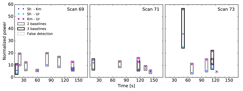
Figure 7: Single pulse detection result of multiple baseline cross matching scheme in Sec. 2.4.1. Single pulses that belongs to the same cross matching group are enclosed by rectangular boxes. Thin and thick lines correspond to single pulses detected on 2 and 3 baselines, respectively. Solid line suggests the time range of the single pulse is overlapped with the pulsar phase range. We name them as “high possibility pulsar signals”. The only false detection is enclosed by rectangular box with dotted line and locates at 122.9 s in scan 73. The corresponding pulsar phase is 0.255. Note that the actual width of the single pulse is much narrower than the width of the rectangular box. The detailed information of 4 single pulses detected on 3 baselines are listed in Tab. 4.

Table 4: Summary of single pulses detected on all 3 baselines.

Scan No.	Baseline	Time	Pulsar	Width	Normalized
		(s)	phase	(ms)	power
	Sh-Km	14.571136	0.978	24.576	5.530
69	Sh-Ur	14.562944	0.966	16.384	3.416
	Km-Ur	14.567040	0.972	8.192	10.243
	Sh-Km	17.546880	0.975	4.096	11.761
71	Sh-Ur	17.548928	0.978	8.192	7.033
	Km-Ur	17.546880	0.975	4.096	14.356
	Sh-Km	49.108608	0.976	4.096	35.642
73	Sh-Ur	49.108608	0.976	4.096	25.115
	Km-Ur	49.108608	0.976	4.096	55.820
	Sh-Km	113.419904	0.974	8.192	10.667
73	Sh-Ur	113.417856	0.971	4.096	7.570
	Km-Ur	113.417856	0.971	4.096	21.318

Fig. 6 present pulse profiles of PSR J0332+5434 after 160 s folding. For 3 stations, Km exhibits the highest power, which is consistent with its antenna performance. Sh is strongly contaminated by RFI which makes it impossible to detect any meaningful signal in single dish mode. The profile of Km and Ur agree well with each other. we can make a raw estimation that the pulsar signal centers at 0.978 with a width of 0.01 in the pulse profile. In this work, a single pulse is assumed to be a “high possibility pulsar signal” if its time range is overlapped with the pulsar phase range (0.973 - 0.983), since its possibility of pulsar origin is much higher than those outside of the pulsar phase range.

3.4 Detection result

In this section, we present the single pulse detection result using two single pulse extraction schemes described Sec. 2.4, and give a brief comparison of two schemes.

3.4.1 Multiple baselines cross matching scheme

We set $N_{\mathrm{win,min}}$ as 3 for all 3 baselines, which means a single pulse is selected as a candidate signal (described in step d of Sec. 2.4.1) if it is detected in 3 or more windows. Then these candidate signals are cross matched on multiple baselines. We present the cross matching result of different baseline combinations in Tab. 3. For single pulses that are detected on at least 1 baseline (column 2, 3, 4), a significant amount of them are those of which the time range is overlapped with the pulsar phase range (number given in the parenthesis of the table). Even for the Sh-Ur baseline of the lowest sensitivity (column 3), the fraction is 10%, which is still tens times larger than the fraction of pulsar phase range among the whole pulsar period (1% according to Fig. 6). This excess can only be explained as single pulses that originate from the pulsar are detected with the cross spectrum method. Therefore, we name those single pulses as “high possibility pulsar signals” and define the detection confidence as the fraction of high possibility pulsar signals among all detected single pulses. For 3 baselines, Km-Ur baseline yields the largest number of single pulses and the highest detection confidence, which is consistent with its high sensitivity. The low sensitivity of Sh antenna (Sheshan 25 m) makes it difficult for single pulse detection on Sh related baselines, and further reduces the number of detected single pulses after cross matching. All single pulses detected on at least 2 baselines are presented in Fig. 7. All of the 4 single pulses detected on 3 baselines are high possibility pulsar signals. For 16 single pulses detected on 2 baselines (those detected on all 3 baselines are excluded), 15 of them are high possibility pulsar signals. Those results demonstrates that single pules detection on 2 or more baselines can almost exclude the possibility of false detection. Note that the normalized power of some single pulses are actually small (less than 5). We detect them by first setting a low threshold to let signals in, then filtering RFIs with multiple windows. Also note that the power of detected single pulses varies one order of magnitude. This is consistent with the observed flux variation of PSR J0332+5434 in Kramer et al. (2003).

3.4.2 Multiple baselines power summation scheme

To improve the detection efficiency, we carry out test of combining the power of several baselines before multiple windows filtering. The result of combining 2 and 3 baselines are presented in Tab. 5. From the data, for the combination of Km-Ur baseline with one of the Sh related baselines (column 6, 7), the detection confidence is slightly enhanced. For the combination of all 3 baselines, the detection confidence does not increase. In both cases, fewer high possibility pulsar signals are detected compared with Km-Ur baseline only. One possible explanation is, we have fewer real pulsar signals that are detectable on low sensitivity baselines. Combining low sensitivity baseline with high sensitivity baseline means in most cases, we actually add noises to signals, and therefore reduce the SNR of high sensitivity baselines. Based on above analysis, it is not necessary to combine high sensitivity baseline with other baselines. On the other side, for the combination of Sh-Km and Sh-Ur baselines (column 5), the detection confidence is greatly enhanced, although this is at the expense of losing 25% of the high possibility pulsar signals. Besides that, compared with the same baseline combination of cross matching scheme, more high possibility pulsar signals are detected. Therefore, this scheme is indeed helpful for extracting weak signals from low sensitivity baselines.

As a summary, two cross spectrum based single pulse extraction schemes exhibit their own pros and cons. The multiple baseline cross matching scheme extracts single pulses with high confidence. However, only a small fraction of single pulses are detectable when the baseline sensitivity is low. The multiple baselines power summation scheme is able to extract more weak signals and enhance detection confidence on the combined low sensitivity baselines.

Table 5: Single pulse detection result with multiple baselines power summation scheme (Sec. 2.4.2). For each scan, we list the number of single pulses detected on the combined baselines (column 5-8). For comparison, single pulses detected on every single baseline are also listed (column 2-4), which are identical to corresponding columns in Tab.3.

Scan No.	1 baseline			2 baselines			3 baselines
	Sh-Km	Sh-Ur	Km-Ur	Sh-Km + Sh-Ur	Sh-Km + Km-Ur	Sh-Ur + km-Ur	Sh-Km + Sh-Ur + Km-Ur
69	37 (12)	33 (2)	49 (40)	15 (9)	42 (35)	41 (33)	40 (34)
71	26 (8)	35 (3)	57 (41)	13 (5)	39 (31)	41 (32)	30 (22)
73	29 (7)	34 (4)	51 (36)	12 (6)	34 (27)	30 (28)	21 (18)

Note. — The number in the parentheses corresponds to single pulses of which the pulse time range is overlapped with the pulsar phase range.

3.5 Localization

In this work, we did not carry out localization for the detected single pulses since it is almost impossible to obtain any reliable result by radio imaging with only 3 points in the UV plane. We have carried out study on the localization of point source using direct solving method, which behaves better under poor UV coverage. The idea is to express the differential phase as a linear function of position offset (Duev et al., 2012):

$$\Delta\phi=f(\Delta\alpha,\Delta\delta)$$ (8)

where $\Delta\phi$ is the differential phase between the phase of target source and the phase of reference source extrapolated to the target time, $\Delta\alpha$ and $\Delta\delta$ are the position offset to the a-priori position of the target source. In theory, above equation is solvable with just two observables. However, the solving process involves phase linking, ambiguity resolving, UV partials calculation, etc. We plan to cover them in our next work.

4 FRB search with VGOS data

The main motivation of this work is to investigate the possibility of FRB search in geodetic VLBI observations. In recent years, the International VLBI Service for Geodesy and Astrometry (IVS) proposed the VLBI2010 Global Observing System (VGOS, Petrachenko et al., 2013), so as to fulfill the requirement of high precision measurement of geodesy and astrometry in the future. To achieve its goal, the whole system are updated, including small telescopes with 12-meter diameter, super wideband data recording system with a sample rate of 16-32 Gbps, linear polarization, etc. On one hand, some features of the VGOS system make it very suitable for FRB search: large field of view (FoV), large number of stations, high frequency and long duration observation sessions. On the other hand, there are still some difficulties we must overcome. In this section, we investigate the possibility of carrying out FRB search in VGOS observation.

4.1 Detection sensitivity

One disadvantage of FRB search with VGOS data is the size of the VGOS antenna is small, which leads to the relatively low sensitivity (SEFD $\sim$ 2000 Jy). However, this can be compensated with its large bandwidth ($\sim$ 0.5 GHz). Based on Eq. 7, and take the SEFD listed in Tab. 7, for a single pulse detected on Sh-Ur baseline with a window length of 4.096 ms and a total bandwidth of 96 MHz, the corresponding average noise level is 0.755 Jy. As demonstrated in panel b of Fig. 4, the standard deviation (fluctuation) of noise is much smaller than the average noise level after fringe fitting. We may set the flux limit as this average noise level. Then a single pulse signal can be easily distinguished from noise fluctuations if its power is larger than this flux limit. To achieve the same noise level for VGOS baselines, the corresponding window length for VGOS baseline is around 7 ms. Therefore, we may expect the sensitivity of VGOS baseline is sufficient for FRB search, if the flux of the single pulse is comparable with single pulses detected on Sh-Ur baseline, and the characteristic width is larger than 7 ms. Finally, we may derive a fluence limit of 5.3 Jy ms for VGOS baseline.

4.2 FFT size

To fully exploit the relatively large FoV of VGOS antenna, we must estimate the appropriate FFT size when carrying out VLBI correlation for FRB search. In appendix B, we have derived the relation of the minimum required FFT size with wavelength $\lambda$, antenna diameter $D$, baseline length $L_{\mathrm{BL}}$ and sampling frequency $f_{\mathrm{s}}$. According to VGOS specification, the 512 MHz bandwidth of each band is divided into 16 frequency channels, which lead to a sample rate of 64 MHz for each frequency channel. Consider a typical VGOS baseline, $\lambda$ $\sim$ 0.136 m (S band, 2.2 GHz), $D$ $\sim$ 12 m, $L_{\mathrm{BL}}$ $\sim$ 3000 km (Shanghai to Urumqi), according to Eq. B1, the minimum FFT size is 3551. We round it to 4096 as a power of 2. The corresponding FFT length is 0.064 ms, which is much shorter than the typical FRB duration, and is therefore acceptable for VLBI correlation in FRB search.

4.3 Detection rate

Keane & Petroff (2015) report an FRB event rate of 2500 events per sky per day above a 1.4 GHz fluence of 2 Jy ms. If we adopt an FRB spectral index $\gamma$ of 0.0 and a fluence index $\alpha$ of -1.0 as discussed in Caleb et al. (2017), the FRB detection rate for VGOS baseline with a fluence limit of 5.3 Jy ms at 2.2 GHz is 0.0076 event per day. We have to point out that above estimation is conservative. First, the predicted FRB event rate is very uncertain. Champion et al. (2016) report the fluence-complete rate above 2 Jy ms is $2.1^{+3.2}_{-1.5}\times 10^{3}$ events per sky per day, which would double the VGOS detection rate if we adopt the upper limit. Besides that, above estimation assumes that antennas only observe one sky area in each scan. However, in real observation, antennas all over the world are usually subdivided into several groups, and observe two or three sky areas simultaneously. Taking these ingredients into account, we may expect an even higher detection rate.

4.4 Fringe fitting

VGOS adopts super wideband data recording system and linear polarization, which requires improved fringe fitting algorithm to achieve its desired measurement precision. Some researchers already start their investigations, e.g, Cappallo (2014); Kondo & Takefuji (2016). Our next step is to combine the advantages of these algorithms and develop high performance fringe fitting algorithm for VGOS cross spectrum of milliseconds duration.

Based on above analysis, we may come to the conclusion that FRB search in VGOS observations is technically feasible. We do expect some exciting discoveries in the VGOS era, and will work on it.

5 Discussion

5.1 High performance implementation

One disadvantage of the cross spectrum based search method is its high computation requirement due to the relatively complex algorithm: we have to carry out fringe fitting independently for a large number of time segments of different window lengths. However, some steps in the fringe fitting scheme can be optimized for a much better performance, which are introduced here.

One may find that the phase rotation by MBD and SBD in Eq. 5 are actually Fourier transforms, which means the searching of MBD and SBD that maximize delay resolution function can be implemented efficiently with a 2 dimensional (2D) fast Fourier transform (FFT, Press et al., 1986). In this case the delay resolution function becomes a matrix, with MBD and SBD take the gridded value $\Delta\tau_{\mathrm{m,g}}$ and $\Delta\tau_{\mathrm{s,g}}$, respectively. The process of maximizing delay resolution function becomes finding the maximum amplitude and the corresponding $\Delta\tau_{\mathrm{m,g}}$, $\Delta\tau_{\mathrm{s,g}}$ in the matrix. The detailed implementation and the discussion of ambiguities are available in Takahashi (2000).

Moreover, we do not fit residual delay rate in the modified fringe fitting scheme. This leads to a good feature of Eq. 5:

$$G_{k_{0},~{}l_{1}}+G_{k_{0}+l_{1},~{}l_{2}}=G_{k_{0},~{}l_{1}+l_{2}},$$ (9)

where $l_{1}$ and $l_{2}$ are window lengths. Above relation also holds for the delay resolution function matrix, which means the matrix of a time segment of large window can be expressed as the direct summation of matrices of several interconnected time segments of small windows. Mathematically above relation is trivial, however it greatly reduces the computation time of fringe fitting for multiple windows in real implementation.

Besides above two optimizations for the algorithm, almost every part of the fringe fitting scheme, including initial phase and channel delay calibration, 2D FFT, amplitude calculation and maximum value localization of the delay resolution matrix, can be implemented in vectorized form. In fact, almost all modern numerical libraries provide support for these operations on different hardware platforms. It is not necessary to implement them from scratch. Moreover, there is no data exchange between time segments during fringe fitting. Therefore, the whole fringe fitting task can be easily divided into multiple small tasks based on time and baseline, and then assigned to multiple hardware processing units. One may fully utilize the computing power of model CPU/GPU clusters in this way.

5.2 Difference with other cross spectrum based methods

Our work is different from other cross spectrum based search methods when it comes to the detailed algorithm and implementation. In Marcote et al. (2017), the arrival times of the bursts were first identified using Arecibo single-dish data. Then the pulse profiles were created with the total power of EVN cross correlations as a function of time. The exact time windows are determined in this way. After that the EVN data are dedispersed and correlated for these time windows. Finally the visibilities are calibrated and used for imaging of single pulses. In Chatterjee et al. (2017), two methods were used to detect bursts with fast-dump visibility data (milliseconds cross spectrum which is similar with time segment in our work) from VLA fast-dump observations. One was milliseconds imaging, which uses the realfast system to search burst in image domain (Law et al., 2015). This method is based on the standard radio imaging pipeline, which involves phase calibration with reference source, 2D Fourier transform from UV plane to image plane, localization of single pulse, etc. (Thompson et al., 2001). Although realfast system already tries to simplify and automatize the whole pipeline, radio imaging is still a complex process and cannot be transplanted to other observation systems easily. Another method was beam-forming analysis, which carries out single pulse search on each synthesized beam. Similar method is used by CHIME, which implements a real-time FFT-beamforming pipeline for FRB search (Ng et al., 2017). Our method can be regarded as an automatic version of the beam search algorithm. The fringe fitting process is somewhat similar with scanning the sky with a virtual beam. The power of the summed cross spectrum reaches maximum when the virtual beam points to the burst position. The difference is, there is no need to set the position of the beam in advance: the beam will find the burst position automatically via fringe fitting.

5.3 Search of dispersion measure

This work does not involve the search of dispersion measure. When constructing time segments in Sec. 3.2, we just use the DM value in the reference. The reason is, the window length in the cross spectrum based method cannot be very small, otherwise the SNR is too low to detect any signal. As a result, this method is not sensitive to DM value. In other words, the DM resolution is low. Here the DM resolution can be estimated with the minimum window length and the frequency range:

$$\mathrm{DM}_{\mathrm{res}}=2.41\times 10^{-7}\times t_{\mathrm{win,~{}min}}~{}/~{}\left(\frac{1}{f_{\mathrm{low}}^{2}}-\frac{1}{f_{\mathrm{high}}^{2}}\right),$$ (10)

where time and frequency take the unit of ms and MHz, respectively. For a single pulse with DM value lower than DM resolution, the difference of arrival time within the frequency range is smaller than the window length. For the VLBI pulsar observation in Sec. 3, the minimum window length of 4.096 ms and a frequency range of 2192 MHz to 2288 MHz yield a DM resolution of 57.7 $\mathrm{pc~{}cm}^{-3}$, which is not enough to resolve the DM value (26.833 $\mathrm{pc~{}cm}^{-3}$) of this pulsar.

One possible solution for DM search in the cross spectrum based method is carried out in two steps:

• Coarse search. The DM search range is partitioned into multiple DM bins according to the DM resolution. For each DM bin, first carry out incoherent dedispersion and construct time segments (Sec. 2.2); then carry out fringe fitting for these time segments (Sec. 2.3) and extract single pulses (Sec. 2.4). For a single pulse detected in several DM bins, pick up the bin that yields the highest signal power.

• Fine search. A DM search with higher DM resolution is carried out inside this DM bin. This can be achieved by either using the cross spectrum based method with higher resolution, or using the auto spectrum based method. The precondition for the latter choice is the signal is strong enough and therefore detectable in the auto spectrum of at least one station.

Consider a typical configuration of FRB search in VGOS observation, we set a minimum window length of 8 ms and a 0.5 GHz bandwidth (2.2 GHz $\sim$ 2.7 GHz). According to Eq. 10, the corresponding DM resolution is 27.8 pc  cm^-3, for the typical 2000 pc cm^-3 DM search range in FRB detection, this requires 72 bins in the coarse search step, which means we have to run 72 times of the FRB search pipeline. As a first look, this requires a large amount of computation. However, as the most time consuming part of the whole pipeline, we already provide a set of high performance implementation for fringe fitting. In particular, our fringe fitting scheme is easy to be parallelized and accelerated with GPU. Therefore, technically, the large DM search range is not a big problem.

6 Summary

In this paper, we introduce our cross spectrum based FRB search method. To test the method, we carry out single pulse search in a VLBI pulsar observation (3 scans, 160 s per scan, 3 geodetic VLBI stations) and validate the result with predicted pulsar phase. The main points of this paper are summarized as follows.

• The cross spectrum method takes the idea of geodetic VLBI data postprocessing and fully utilizes the fringe phase information to maximize the power of single pulse signals. To exclude RFI and achieve a higher detection confidence, candidate signals are filtered in multiple windows and cross matched on multiple baselines. Moreover, the power of multiple baselines are combined to improve detection sensitivity.

• According to our test, single pulses detected on 2 or more baselines can almost exclude the possibility of RFIs. By combining the power of multiple baselines, a greater number of weak signals are extracted from low sensitivity baselines with higher confidence.

• The whole pipeline is easy to implement and parallelize, which can be deployed in various kinds of VLBI observations. In particular, we point out VGOS observations are very suitable for FRB search.

Appendix A Initial phase and channel delay extraction

The extraction of initial phase and channel delay can be summarized in the following steps.

• Setting $\phi_{0}^{n}$ and $\Delta\tau_{0}^{n}$ as 0.

• Constructing a time segment with a window length of several seconds for the calibration source.

• Carrying out fringe fitting on this time segment and finding out $\Delta\tau_{\mathrm{m}}$ and $\Delta\tau_{\mathrm{s}}$ that maximize delay resolution function. The initial phase of frequency channel $n$ is derived by:

  $$\phi_{0}^{n}=\angle\sum_{j=1}^{J-1}S_{k_{0},~{}l}(n,j)e^{-i2\pi\left[f_{j}\Delta\tau_{\mathrm{s}}+(f_{0}^{n}-f_{\mathrm{ref,fit}})\Delta\tau_{\mathrm{m}}\right]}.$$ (A1)

  The channel delay $\Delta\tau_{0}^{n}$ is derived by fitting $S_{k_{0},~{}l}(n,j)e^{-i2\pi f_{j}\Delta\tau_{\mathrm{s}}}$.

The initial phase extraction method introduced here is similar with the “manual” mode in HOPS. One may use the PCAL signal extracted by HOPS directly.

Appendix B Estimation of FFT size

Since delay models are calculated for the center of the FoV, a source that does not appear in the center of FoV will lead to an extra delay $\Delta\tau$, which varies from $-\Delta\tau_{\mathrm{max}}$ to $\Delta\tau_{\mathrm{max}}$. The maximum delay $\Delta\tau_{\mathrm{max}}$ is achieved when the source appears at the edge of the main beam. The size of the main beam (angular diameter) can be estimated with the full width at half maximum: $\theta_{\mathrm{FWHM}}\sim\lambda/D$. Here $\lambda$ is the wavelength, $D$ is the antenna diameter. Then $\Delta\tau_{\mathrm{max}}$ can be estimated with: $\Delta\tau_{\mathrm{max}}\sim\frac{1}{2}\theta_{\mathrm{FWHM}}~{}L_{\mathrm{BL}}/c$. Here $L_{\mathrm{BL}}$ is the baseline length.

In the FX type correlator, two time series are first Fourier transformed to frequency domain via FFT with size $N$, the corresponding frequency points are conjugate multiplied. The cross spectrum is obtained in this way with frequency resolution $f_{\mathrm{s}}/N$. Here $f_{\mathrm{s}}$ is the sampling rate of each frequency channel. In general, for each frequency channel, the cross spectrum with frequency resolution $f_{\mathrm{s}}/N$ corresponds to the SBD search range from $-\frac{N}{2}~{}T_{\mathrm{s}}$ to $\frac{N}{2}~{}T_{\mathrm{s}}$. Here $T_{\mathrm{s}}$ is the sampling time: $T_{\mathrm{s}}=1/f_{\mathrm{s}}$. When searching for SBD in the real fringe fitting scheme, the cross spectrum will be zero padded to achieve a higher time resolution.

To make the source detectable, the SBD search range in the fringe fitting scheme must cover the maximum delay: $\frac{N}{2}T_{\mathrm{s}}\geq\Delta\tau_{\mathrm{max}}$. Finally we get the minimum required FFT size:

$$N_{\mathrm{min}}=\frac{\lambda}{D}\frac{L_{\mathrm{BL}}}{c}f_{\mathrm{s}}.$$ (B1)

References

- (1)
- Altamimi et al. (2016) Altamimi, Z., Rebischung, P., Métivier, L., & Collilieux, X. 2016, Journal of Geophysical Research (Solid Earth), 121, 6109
- Bassa et al. (2017) Bassa, C. G., Tendulkar, S. P., Adams, E. A. K., et al. 2017, ApJ, 843, L8
- Behrend (2013) Behrend, D. 2013, Data Science Journal, 12, WDS81
- Burke-Spolaor et al. (2016) Burke-Spolaor, S., Trott, C. M., Brisken, W. F., et al. 2016, ApJ, 826, 223
- Caleb et al. (2016) Caleb, M., Flynn, C., Bailes, M., et al. 2016, MNRAS, 458, 718
- Caleb et al. (2017) Caleb, M., Flynn, C., Bailes, M., et al. 2017, MNRAS, 468, 3746
- Cappallo (2014) Cappallo, R. 2014, International VLBI Service for Geodesy and Astrometry 2014 General Meeting Proceedings: “VGOS: The New VLBI Network”, Eds. Dirk Behrend, Karen D. Baver, Kyla L. Armstrong, Science Press, Beijing, China, ISBN 978-7-03-042974-2, 2014, p. 91-96, 91
- Cappallo (2016) Cappallo, R. 2016, International VLBI Service for Geodesy and Astrometry 2016 General Meeting Proceedings: “New Horizons with VGOS”, Eds. Dirk Behrend, Karen D. Baver, Kyla L. Armstrong, NASA/CP-2016-219016, p. 61-64, 61
- Champion et al. (2016) Champion, D. J., Petroff,
- Chatterjee et al. (2017) Chatterjee, S., Law, C. J., Wharton, R. S., et al. 2017, Nature, 541, 58
- Chen et al. (2015) Chen, W., Jiang, W., Li, Z. X., Xu, Y. H., & Wang, M. 2015, Acta Astronomica Sinica, 56, 658
- Cotton (1995) Cotton, W. D. 1995, Very Long Baseline Interferometry and the VLBA, 82, 189
- Dai et al. (2016) Dai, Z. G., Wang, J. S., Wu, X. F., & Huang, Y. F. 2016, ApJ, 829, 27
- Deller et al. (2011) Deller, A. T., Brisken, W. F., Phillips, C. J., et al. 2011, PASP, 123, 275
- Deller et al. (2007) Deller, A. T., Tingay, S. J., Bailes, M., & West, C. 2007, PASP, 119, 318
- Duev et al. (2012) Duev, D. A., Molera Calvés, G., Pogrebenko, S. V., et al. 2012, A&A, 541, A43
- Falcke & Rezzolla (2014) Falcke, H., & Rezzolla, L. 2014, A&A, 562, A137
- Fish et al. (2016) Fish, V. L., Johnson, M. D., Doeleman, S. S., et al. 2016, ApJ, 820, 90
- Geng & Huang (2015) Geng, J. J., & Huang, Y. F. 2015, ApJ, 809, 24
- Hu (2008) Hu, X. 2008, 37th COSPAR Scientific Assembly, 37, 1284
- Hobbs et al. (2006) Hobbs, G. B., Edwards, R. T., & Manchester, R. N. 2006, MNRAS, 369, 655
- Kashiyama et al. (2013) Kashiyama, K., Ioka, K., & Mészáros, P. 2013, ApJ, 776, L39
- Katz (2016a) Katz, J. I. 2016a, Modern Physics Letters A, 31, 1630013
- Katz (2016b) Katz, J. I. 2016b, ApJ, 818, 19
- Katz (2016c) Katz, J. I. 2016c, ApJ, 826, 226
- Keane et al. (2016) Keane, E. F., Johnston, S., Bhandari, S., et al. 2016, Nature, 530, 453
- Keane & Petroff (2015) Keane, E. F., & Petroff, E. 2015, MNRAS, 447, 2852
- Keane et al. (2012) Keane, E. F., Stappers, B. W., Kramer, M., & Lyne, A. G. 2012, MNRAS, 425, L71
- Keimpema et al. (2015) Keimpema, A., Kettenis, M. M., Pogrebenko, S. V., et al. 2015, Experimental Astronomy, 39, 259
- Kondo & Takefuji (2016) Kondo, T., & Takefuji, K. 2016, Radio Science, 51, 1686
- Kramer et al. (2003) Kramer, M., Karastergiou, A., Gupta, Y., et al. 2003, A&A, 407, 655
- Law et al. (2015) Law, C. J., Bower, G. C., Burke-Spolaor, S., et al. 2015, ApJ, 807, 16
- Lorimer et al. (2007) Lorimer, D. R., Bailes, M., McLaughlin, M. A., Narkevic, D. J., & Crawford, F. 2007, Science, 318, 777
- Lorimer & Kramer (2004) Lorimer, D. R., & Kramer, M. 2004, Handbook of pulsar astronomy, by D.R. Lorimer and M. Kramer. Cambridge observing handbooks for research astronomers, Vol. 4. Cambridge, UK: Cambridge University Press
- Ma et al. (2009) Ma, C., Arias, E. F., Bianco, G., et al. 2009, IERS Technical Note, 35,
- Ma et al. (1998) Ma, C., Arias, E. F., Eubanks, T. M., et al. 1998, AJ, 116, 516
- Manchester et al. (2005) Manchester, R. N., Hobbs, G. B., Teoh, A., & Hobbs, M. 2005, AJ, 129, 1993
- Marcote et al. (2017) Marcote, B., Paragi, Z., Hessels, J. W. T., et al. 2017, ApJ, 834, L8
- Masui et al. (2015) Masui, K., Lin, H.-H., Sievers, J., et al. 2015, Nature, 528, 523
- McLaughlin et al. (2007) McLaughlin, M. A., Rea, N., Gaensler, B. M., et al. 2007, ApJ, 670, 1307
- Mottez & Zarka (2014) Mottez, F., & Zarka, P. 2014, A&A, 569, A86
- Ng et al. (2017) Ng, C., Vanderlinde, K., Paradise, A., et al. 2017, arXiv:1702.04728
- Paragi (2016) Paragi, Z. 2016, arXiv:1612.00508
- Pen & Connor (2015) Pen, U.-L., & Connor, L. 2015, ApJ, 807, 179
- Petrachenko et al. (2013) Petrachenko, W., Behrend, D., Hase, H., et al. 2013b, EGU General Assembly Conference Abstracts, 15, EGU2013-12867
- Press et al. (1986) Press, W. H., Flannery, B. P., & Teukolsky, S. A. 1986, Cambridge: University Press, 1986,
- Ransom (2001) Ransom, S. M. 2001, Ph.D. Thesis
- Rogers et al. (1983) Rogers, A. E. E., Cappallo, R. J., Hinteregger, H. F., et al. 1983, Science, 219, 51
- Scholz et al. (2017) Scholz, P., Bogdanov, S., Hessels, J. W. T., et al. 2017, ApJ, 846, 80
- Scholz et al. (2016) Scholz, P., Spitler, L. G., Hessels, J. W. T., et al. 2016, ApJ, 833, 177
- Schuh & Behrend (2012) Schuh, H., & Behrend, D. 2012, Journal of Geodynamics, 61, 68
- Shu et al. (2009) Shu, F., Zheng, W., Zhang, X., et al. 2009, 19th European VLBI for Geodesy and Astrometry Working Meeting, 87
- Spitler et al. (2016) Spitler, L. G., Scholz, P., Hessels, J. W. T., et al. 2016, Nature, 531, 202
- Takahashi (2000) Takahashi, H., et al., 2000, “Wave Summit Course: Very Long Baseline Interferometer.” Ohmsha. Ltd.
- Tendulkar et al. (2017) Tendulkar, S. P., Bassa, C. G., Cordes, J. M., et al. 2017, ApJ, 834, L7
- Thompson et al. (2001) Thompson, A. R., Moran, J. M., & Swenson, G. W., Jr. 2001, “Interferometry and synthesis in radio astronomy by A. Richard Thompson, James M. Moran, and George W. Swenson, Jr. 2nd ed. New York : Wiley, c2001.xxiii, 692 p. : ill. ; 25 cm. ”A Wiley-Interscience publication.“ Includes bibliographical references and indexes. ISBN : 0471254924”,
- Thompson et al. (2011) Thompson, D. R., Wagstaff, K. L., Brisken, W. F., et al. 2011, ApJ, 735, 98
- Thornton et al. (2013) Thornton, D., Stappers, B., Bailes, M., et al. 2013, Science, 341, 53
- Wang et al. (2016) Wang, J.-S., Yang, Y.-P., Wu, X.-F., Dai, Z.-G., & Wang, F.-Y. 2016, ApJ, 822, L7
- Wayth et al. (2011) Wayth, R. B., Brisken, W. F., Deller, A. T., et al. 2011, ApJ, 735, 97
- Whitney (2003) Whitney, A. R. 2003, New technologies in VLBI, 306, 123
- Whitney et al. (2009) Whitney, A., Kettenis, M., Phillips, C., & Sekido, M. 2009, 8th International e-VLBI Workshop, 42
- Whitney et al. (1976) Whitney, A. R., Rogers, A. E. E., Hinteregger, H. F., et al. 1976, Radio Science, 11, 421
- Zhang (2014) Zhang, B. 2014, ApJ, 780, L21
- Zheng (2015) Zheng, W. 2015, IAU General Assembly, 22, 2255896
- Zheng et al. (2014) Zheng, W., Huang, Y., Chen, Z., et al. 2014, International VLBI Service for Geodesy and Astrometry 2014 General Meeting Proceedings: “VGOS: The New VLBI Network”, Eds. Dirk Behrend, Karen D. Baver, Kyla L. Armstrong, Science Press, Beijing, China, ISBN 978-7-03-042974-2, 2014, p. 466-472, 466
- Zheng et al. (2010) Zheng, W., Quan, Y., Shu, F., et al. 2010, Sixth International VLBI Service for Geodesy and Astronomy. Proceedings from the 2010 General Meeting, “VLBI2010: From Vision to Reality”. Held 7-13 February, 2010 in Hobart, Tasmania, Australia. Edited by D. Behrend and K.D. Baver. NASA/CP 2010-215864., p.157-161, 157
- Zheng et al. (2007) Zheng, W., Shu, F., & Zhang, D. 2007, Proc. SPIE, 6795, 67954N
- Zhu et al. (2016) Zhu, R., Wu, Y., & Li, J. 2016, International VLBI Service for Geodesy and Astrometry 2016 General Meeting Proceedings: “New Horizons with VGOS”, Eds. Dirk Behrend, Karen D. Baver, Kyla L. Armstrong, NASA/CP-2016-219016, p. 163-165, 163