Linear-Quadratic Mean Field Control: The Hamiltonian Matrix
and Invariant Subspace Method

Abstract

This paper studies the existence and uniqueness of a solution to linear quadratic (LQ) mean field social optimization problems with uniform agents. We exploit a Hamiltonian matrix structure of the associated ordinary differential equation (ODE) system and apply a subspace decomposition method to find the solution. This approach is effective for both the existence analysis and numerical computations. We further extend the decomposition method to LQ mean field games.

I Introduction

Mean field game (MFG) theory studies stochastic dynamic decision problems involving a large number of noncooperative and individually insignificant agents, and provides a powerful methodology to reduce the complexity in designing strategies [13]. For an overview of the theory and applications, the readers are referred to [4, 7, 12, 14, 16, 19] and references therein.

There has existed a parallel development on mean field social optimization where a large number of agents cooperatively minimize a social cost as the sum of individual costs. Different from mean field games, the individual strategy selection of an agent is not selfish and should take into account both self improvement and the aggregate impact on other agents’ costs. Mean field social optimization problems have been studied in multi-agent collective motion [1, 28], social consensus control [25], economic theory [26]. Other related literature includes Markov decision processes using aggregate statistics and their mean field limit [11], LQ mean field teams [2], LQ social optimization with a major player [17], mean field teams with Markov jumps [31], social optimization with nonlinear diffusion dynamics [30], and cooperative stochastic differential games [34].

In this paper, we consider social optimization in an LQ model of uniform agents. The dynamics of agent $i$ are given by the stochastic differential equation (SDE):

$$dx_{i}=(Ax_{i}+Bu_{i})dt+DdW_{i},\quad t\geq 0,\quad 1\leq i\leq N.$$ (1)

The state $x_{i}$ and the control $u_{i}$ are $n$ and $n_{1}$ dimensional vectors respectively. The initial states $\{x_{i}(0),\ 1\leq i\leq N\}$ are independent. The noise processes $\{W_{i},\ 1\leq i\leq N\}$ are $n_{2}$ dimensional independent standard Brownian motions, which are also independent of $\{x_{i}(0),\ 1\leq i\leq N\}$. The constant matrices $A$, $B$ and $D$ have compatible dimensions. Given a symmetric matrix $M\geq 0$, the quadratic form $z^{T}Mz$ is sometimes denoted by $|z|_{M}^{2}$. Denote $u:=(u_{1},\cdots,u_{N})$.

The individual cost for agent $i$ is given by

$$J_{i}(u(\cdot))=E\int_{0}^{\infty}e^{-\rho t}[|x_{i}-\Phi(x^{(N)})|_{Q}^{2}+u_{i}^{T}Ru_{i}]dt,$$ (2)

where $\rho>0$, $\Phi(x^{(N)})=\Gamma x^{(N)}+\eta$ and $x^{(N)}:=(1/N)\sum_{i=1}^{N}x_{i}$ is the mean field coupling term. The constant matrices or vectors $\Gamma$, $Q$, $R$ and $\eta$ have compatible dimensions, and $Q$, $R$ are symmetric. The social cost is defined as

$$J_{\rm soc}^{(N)}(u(\cdot))=\sum_{i=1}^{N}J_{i}(u(\cdot)).$$

The minimization of the social cost is an optimal control problem. However, the exact solution requires centralized information for each agent. So a solution of practical interest is to find a set of decentralized strategies which has negligible optimality loss in minimizing $J_{\rm soc}^{(N)}(u(\cdot))$ for large $N$ and the solution method has been developed in [15] under the following assumption: (A1) $Q\geq 0$, $R>0$, $(A,B)$ is stabilizable and $(A,Q^{\frac{1}{2}})$ is detectable.

Under (A1), there exists a unique solution $\Pi\geq 0$ to the algebraic Riccati equation (ARE):

$$\rho\Pi=\Pi A+A^{T}\Pi-\Pi BR^{-1}B^{T}\Pi+Q.$$ (3)

Denote $Q_{\Gamma}=\Gamma^{T}Q+Q\Gamma-\Gamma^{T}Q\Gamma$ and $\eta_{\Gamma}=(I-\Gamma^{T})Q\eta$. We introduce the Social Certainty Equivalence (SCE) equation system:

$$\frac{d\bar{x}}{dt}=(A-BR^{-1}B^{T}\Pi)\bar{x}-BR^{-1}B^{T}s,$$ (4)

$$\frac{ds}{dt}=Q_{\Gamma}\bar{x}+(\rho I-A^{T}+\Pi BR^{-1}B^{T})s+\eta_{\Gamma},$$ (5)

where $\bar{x}(0)=x_{0}$ is given and $s(0)=s_{0}$ is to be determined. We look for $(\bar{x},s)\in C_{\rho/2}([0,\infty),\mathbb{R}^{2n})$ (see Definition 2). If a finite time horizon $[0,T]$ is considered for (2), $s$ will have a terminal condition $s(T)$ and $\Pi$ will depend on time. This results in a standard two point boundary value (TPBV) problem for linear ordinary differential equations (ODEs). Given the infinite horizon, $s$ satisfies a growth condition instead of a terminal condition.

The key result in [15] under (A1) is that if (4)-(5) has a unique solution, the set of decentralized strategies

$$\hat{u}_{i}=-R^{-1}B^{T}(\Pi x_{i}+s),\quad 1\leq i\leq N,$$ (6)

has asymptotic social optimality. In other words, centralized strategies can further reduce the cost $J_{\rm soc}^{(N)}(u(\cdot))$ by at most $o(N)$. In fact, [15] constructed a more general version of (4)-(5) where the parameter $A$ is randomized over the population and accordingly $\bar{x}$ in the equation of $s$ is replaced by a mean field averaging over the nonuniform population.

I-A Our Approach and Contributions

After some transformation, the coefficient matrix of (4)-(5) reduces to a Hamiltonian matrix which can be associated with an LQ optimal control problem with state weight matrix $-Q_{\Gamma}$. The connection to such an LQ control problem is remarkable since its state weight may not be positive semi-definite. When $Q_{\Gamma}\leq 0$, existence and uniqueness of the solution has been proved [15, Theorem 4.3] by a standard Riccati equation approach. On the other hand, due to the intrinsic optimal control nature of the social optimization problem, one expects to obtain solvability of the SCE equation system under much more general conditions, which is the focus of this work. Furthermore, our approach allows $Q$ to be indefinite. LQ optimal control problems with indefinite state and/or control weight is a subject of considerable interest [10, 29, 32, 36].

We develop a new approach to analyze and compute the solution of (4)-(5) for a general $Q_{\Gamma}$ by exploiting a Hamiltonian matrix structure and the well known invariant subspace method [6]. Specifically, aided by the solution of a continuous-time algebraic Riccati equation (ARE) with possibly indefinite state weight, we decompose the Hamiltonian matrix into a block-wise triangular form where the stable eigenvalues are separated from the unstable ones. To numerically solve the Riccati equation, we apply the Schur method [20]. The approach of decomposing the stable invariant subspace is further extended to solve LQ mean field games; see [3, 5, 21, 23] for related literature on LQ mean field games. The main results of this paper have been reported in [8, 9] in an early form.

The organization of the paper is as follows. Section II proves existence and uniqueness of a solution to the SCE equation system and develops a computational method. Section III extends the analysis to LQ mean field games. Numerical examples are presented in Section IV. Section V concludes the paper.

II Solution of the Social Optimization Problem

II-A Preliminaries on Algebraic Riccati Equations

Let $S^{n}\subset\mathbb{R}^{n\times n}$ denote the set of symmetric matrices, and $S^{n}_{+}\subset S^{n}$ the set of positive semi-definite matrices. Our later analysis depends on an invariant subspace decomposition method which involves a class of continuous-time algebraic Riccati equations (ARE) of the form

$$XA_{o}+A_{o}^{T}X-XMX+Q_{o}=0,$$ (7)

where $A_{o}$, $Q_{o}$, $M$ are given matrices in $\mathbb{R}^{n\times n}$ with $Q_{o}\in S^{n}$ and $M\in S^{n}_{+}$. Note that $Q_{o}$ is not required to be positive semi-definite. Denote the Hamiltonian matrix

$$H_{o}=\begin{bmatrix}A_{o}&-M\\ -Q_{o}&-A_{o}^{T}\\ \end{bmatrix}.$$ (8)

Note that the eigenvalues of a Hamiltonian matrix are distributed symmetrically about both the real axis and the imaginary axis [22]. If $H_{o}$ has no eigenvalue on the imaginary axis, the left and right open half planes each contain $n$ eigenvalues.

For a solution $X_{+}\in S^{n}$ of (7), $X_{+}$ is the maximal real symmetric solution [18] if for any solution $X\in S^{n}$, $X_{+}-X\geq 0$. A (real or complex) matrix is called stable if all its eigenvalues are in the open left half-plane; such an eigenvalue is also said to be stable.

Proposition 1

If $(A_{o},M)$ is stabilizable and $H_{o}$ has no eigenvalues on the imaginary axis (i.e., no eigenvalues with zero real parts), then there exists a unique maximal real symmetric solution $X_{+}$ and $A_{o}-MX_{+}$ is stable.

Proof:

By Theorem 9.3.1 in [18, p. 239], there exists a unique almost stabilizing solution $X$ in $S^{n}$ (i.e., all eigenvalues of $A_{o}-MX$ are in the closed left half plane). Further applying Theorem 7.9.4 in [18, p. 195-196], we obtain a unique maximal real symmetric solution $X_{+}$ and $A_{o}-MX_{+}$ is stable. ∎

II-B The Transformation

Definition 2

For integer $k\geq 1$ and real number $r>0$, $C_{r}([0,\infty),\mathbb{R}^{k})$ consists of all functions $f\in C([0,\infty),\mathbb{R}^{k})$ such that $\sup_{t\geq 0}|f(t)|e^{-r^{\prime}t}<\infty$, for some $0<r^{\prime}<r$. Here $r^{\prime}$ may depend on $f$.

Denote

$$H_{A}=\begin{bmatrix}A-\frac{\rho}{2}I&-BR^{-1}B^{T}\\ -Q&-A^{T}+\frac{\rho}{2}I\\ \end{bmatrix}.\$$ (9)

We introduce the following standing assumption for the rest of this paper.

(SA) $(A,B)$ is stabilizable, $R>0$, and $H_{A}$ has no eigenvalues with zero real parts.

Under (SA), we may solve a unique maximal solution $\Pi\in S^{n}$ from (3) such that $A-BR^{-1}B^{T}\Pi-\frac{\rho}{2}I$ is stable. This ensures the construction of (4)-(5). Note that we do not require $Q\geq 0$.

Define

$$\tilde{x}=e^{-\rho t/2}\bar{x},\quad\tilde{s}=e^{-\rho t/2}s.$$

We obtain

$$\begin{bmatrix}\frac{d\tilde{x}}{dt}\\ \frac{d\tilde{s}}{dt}\\ \end{bmatrix}=H\begin{bmatrix}\tilde{x}\\ \tilde{s}\\ \end{bmatrix}+\begin{bmatrix}0\\ \tilde{\eta}_{\Gamma}\\ \end{bmatrix},$$ (10)

where $\tilde{x}(0)=x_{0}$, $\tilde{\eta}_{\Gamma}=e^{-\frac{\rho}{2}t}\eta_{\Gamma}$, and

$$H=\begin{bmatrix}\mathcal{A}&-BR^{-1}B^{T}\\ Q_{\Gamma}&-\mathcal{A}^{T}\\ \end{bmatrix},\ \mathcal{A}=A-BR^{-1}B^{T}\Pi-\frac{\rho}{2}I.$$ (11)

Note that $\tilde{\eta}_{\Gamma}$ in (10) is a function of $t$. Since $Q_{\Gamma}$ is symmetric, $H$ is a Hamiltonian matrix.

II-C Existence and Uniqueness of a Solution

Consider the general matrix differential equation

$$\frac{dz}{dt}=Kz+\psi(t),$$ (12)

where $z=[z_{1}^{T},z_{2}^{T}]^{T}$, $z_{1},z_{2}\in\mathbb{R}^{n}$, $K\in\mathbb{R}^{2n\times 2n}$ and for some $C>0$, $|\psi(t)|\leq Ce^{-\frac{\rho t}{2}}$ for all $t\geq 0$, and where $z_{1}(0)$ is given.

Definition 3

The matrix $K\in\mathbb{R}^{2n\times 2n}$ is said to satisfy condition (H0) if there exists an invertible real matrix $U=(U_{ij})_{1\leq i,j\leq 2}$, where $U_{11}\in\mathbb{R}^{n\times n}$ is invertible, such that

$$U^{-1}KU=\begin{bmatrix}F_{11}&F_{12}\\ 0&F_{22}\\ \end{bmatrix},$$

where $F_{11}$ and $-F_{22}$ are $n\times n$ stable matrices.

Let $M_{1}$ be an $(n+m)\times(n+m)$ real (or complex) matrix which has an $n$-dimensional invariant subspace ${\mathcal{V}}$. If ${\mathcal{V}}$ is spanned by the columns of an $(n+m)\times n$ matrix whose leading $n\times n$ sub-matrix is invertible, ${\mathcal{V}}$ is called a graph subspace [6, 18].

Remark 1

A matrix $K$ satisfying (H0) has $n$ stable eigenvalues and the associated $n$-dimensional stable invariant subspace of $K$ is a graph subspace.

Lemma 4

Suppose $K$ in (12) satisfies (H0). Then for the given $z_{1}(0)$, there exists a unique

$$z_{2}(0)= U_{21}U_{11}^{-1}z_{1}(0)$$

$$+(U_{21}U_{11}^{-1}U_{12}-U_{22})\int_{0}^{\infty}e^{-F_{22}\tau}[V_{21},V_{22}]\psi(\tau)d\tau$$

such that (12) has a bounded solution on $[0,\infty)$, where $V=U^{-1}=(V_{ij})_{1\leq i,j\leq 2}$. In this case, for some $\epsilon_{0}>0$, $z(t)e^{\varepsilon_{0}t}$ is still bounded on $[0,\infty)$.

Proof:

For (12), we apply a change of variable to define

$$y=U^{-1}z,$$ (13)

where $y=[y_{1}^{T},y_{2}^{T}]^{T}$, $y_{i}\in\mathbb{R}^{n}$. We have

$$\frac{dy_{1}}{dt}=F_{11}y_{1}+F_{12}y_{2}+\varphi_{1}(t),$$ (14)

$$\frac{dy_{2}}{dt}=F_{22}y_{2}+\varphi_{2}(t),$$ (15)

where $U^{-1}\psi=[\varphi_{1}^{T},\varphi_{2}^{T}]^{T}$. We proceed to find a bounded solution $y$. Since $-F_{22}$ is stable, there is a unique choice of

$$y_{2}(0)=-\int_{0}^{\infty}e^{-F_{22}\tau}\varphi_{2}(\tau)d\tau$$

such that $y_{2}(t)=-\int_{t}^{\infty}e^{F_{22}(t-\tau)}\varphi_{2}(\tau)d\tau$ is bounded, which further determines a bounded $y_{1}$ regardless of $y_{1}(0)$. Using the relation (13) at $t=0$, we next uniquely determine

$$y_{1}(0)=U_{11}^{-1}[z_{1}(0)-U_{12}y_{2}(0)].$$ (16)

Finally, we obtain $z_{2}(0)=U_{21}y_{1}(0)+U_{22}y_{2}(0)$, which gives a bounded solution $z$ of (12) on $[0,\infty)$. It can be checked that for some $\epsilon_{0}>0$, $z(t)e^{\varepsilon_{0}t}$ is still bounded on $[0,\infty)$.

The choice of $z_{2}(0)$ is unique since otherwise by (13) we may construct two different bounded solutions $y\neq\hat{y}$, where we necessarily have $y_{1}(0)\neq\hat{y}_{1}(0)$, $y_{2}(0)=\hat{y}_{2}(0)$, which is impossible in view of (16). ∎

The proof of the existence result in the theorem below reduces to showing the stable invariant subspace of $H$ is a graph subspace.

Theorem 5

Assume that the pair $(A,B)$ is stabilizable and the Hamiltonian matrix $H$ in (11) has no eigenvalues with zero real parts. Then there exists a unique initial condition $s_{0}$ such that (4)-(5) has a solution $(\bar{x},s)\in C_{\rho/2}([0,\infty),\mathbb{R}^{2n})$.

Proof:

Since $\mathcal{A}$ is stable, both $({\mathcal{A}},B)$ and $(\mathcal{A},BR^{-1}B^{T})$ are stabilizable [33]. Consider the ARE

$$X\mathcal{A}+\mathcal{A}^{T}X-XBR^{-1}B^{T}X-Q_{\Gamma}=0.$$ (17)

By Corollary 1, there exists a unique maximal real symmetric solution $X_{+}$ such that $\mathcal{A}-BR^{-1}B^{T}X_{+}$ is stable. Denote $U=\begin{bmatrix}I&0\\ X_{+}&I\end{bmatrix}$. So $U^{-1}=\begin{bmatrix}I&0\\ -X_{+}&I\end{bmatrix}.$ Then

$$U^{-1}HU =\begin{bmatrix}I&0\\ -X_{+}&I\end{bmatrix}\begin{bmatrix}\mathcal{A}&-BR^{-1}B^{T}\\ Q_{\Gamma}&-\mathcal{A}^{T}\\ \end{bmatrix}\begin{bmatrix}I&0\\ X_{+}&I\end{bmatrix}$$

$$=\begin{bmatrix}\mathcal{A}_{C}&-BR^{-1}B^{T}\\ 0&-\mathcal{A}_{C}^{T}\end{bmatrix},$$

where $\mathcal{A}_{C}=\mathcal{A}-BR^{-1}B^{T}X_{+}$ is stable. By Lemma 4, after selecting the initial condition $s_{0}=X_{+}x_{0}-\int_{0}^{\infty}e^{\mathcal{A}^{T}_{C}\tau}\eta_{\Gamma}e^{-\rho\tau/2}d\tau$, the resulting solution $(\bar{x},s)\in C_{\rho/2}([0,\infty),\mathbb{R}^{2n})$. And $s_{0}$ is unique. ∎

For the special case $Q_{\Gamma}\leq 0$, since ${\mathcal{A}}$ is stable, (17) has a unique positive semi-definite solution $X$ by the standard theory of Riccati equations [33]. On the other hand, by [18, Theorem 9.3.3], in this case $H$ necessarily has no eigenvalues with zero real parts.

Example 1

Consider a scalar model with $A=a$, $B=b\neq 0$, $R=r>0$, $Q=q>0$, $\Gamma=\gamma$. Then $Q_{\Gamma}=(2\gamma-\gamma^{2})q$. Denote $a_{\rho}=a-\rho/2$ and $b_{r}=b/\sqrt{r}$. We solve the Riccati equation $\rho\Pi=2a\Pi-b^{2}\Pi/r+q$ to obtain $\Pi=(a_{\rho}+\sqrt{a_{\rho}^{2}+qb_{r}^{2}})/b_{r}^{2}$. Then $H$ in (11) becomes

$$H=\begin{bmatrix}-\sqrt{a_{\rho}^{2}+qb_{r}^{2}}&-b_{r}^{2}\\ (2\gamma-\gamma^{2})q&\sqrt{a_{\rho}^{2}+qb_{r}^{2}}\end{bmatrix}.$$

The characteristic equation $\det(\lambda I-H)=0$ reduces to $\lambda^{2}=a_{\rho}^{2}+qb_{r}^{2}(1-\gamma)^{2}$. Therefore, $H$ has eigenvalues with zero real parts if and only if $a=\rho/2$ and $\gamma=1$ when $b\neq 0$ and $q>0$.

Example 2

We continue with the system in Example 1 for the case $a=\rho/2$ and $\gamma=1$. The SCE equation system now becomes

$$\begin{bmatrix}\dot{\bar{x}}(t)\\ \dot{s}(t)\end{bmatrix}=\begin{bmatrix}\frac{\rho}{2}-\sqrt{q}|b_{r}|&-b_{r}^{2}\\ q&\frac{\rho}{2}+\sqrt{q}|b_{r}|\end{bmatrix}\begin{bmatrix}{\bar{x}}(t)\\ s(t)\end{bmatrix},$$

where $\bar{x}(0)$ is given. We obtain the solution

$$\begin{bmatrix}{\bar{x}}(t)\\ s(t)\end{bmatrix}=e^{\frac{\rho t}{2}}\begin{bmatrix}1-\sqrt{q}|b_{r}|t&-b_{r}^{2}t\\ qt&1+\sqrt{q}|b_{r}|t\end{bmatrix}\begin{bmatrix}{\bar{x}}(0)\\ s(0)\end{bmatrix},$$

which is not in $C_{\rho/2}([0,\infty),\mathbb{R}^{2})$ unless $\bar{x}(0)=s(0)=0$.

Example 3

Consider the system given in Example 2. We have $\Pi=\sqrt{q}/|b_{r}|$, ${\mathcal{A}}=-\sqrt{q}|b_{r}|$, $Q_{\Gamma}=q$. The Riccati equation (17) now has the solution $X=-\sqrt{q}/|b_{r}|<0$, and ${\mathcal{A}}-b_{r}^{2}X=0$ implying $X$ being almost stabilizing, which is due to the two zero eigenvalues of $H$.

II-D Computational Methods for the ARE

Consider ARE (7). Let $H_{o}$ be defined by (8). This part describes the numerical method for a stabilizing solution when $Q_{o}$ may not be positive semi-definite. Denote

$$W=\begin{bmatrix}U_{1}\\ U_{2}\end{bmatrix}\in\mathbb{C}^{2n\times n}.$$

Proposition 6

Suppose i) $H_{o}$ has no eigenvalues with zero real parts and

$$H_{o}\begin{bmatrix}U_{1}\\ U_{2}\end{bmatrix}=\begin{bmatrix}U_{1}\\ U_{2}\end{bmatrix}S_{o},$$ (18)

where $S_{o}$ is stable; ii) $(A_{o},M)$ is stabilizable. Then $U_{1}$ is invertible and $U_{2}U_{1}^{-1}$ is real, symmetric and satisfies (7), and $A_{o}-MU_{2}U_{1}^{-1}$ is stable.

Proof:

This proposition holds as a corollary to Theorems 13.5 and 13.6 in [35] under condition ii). In this case the invariant subspace of $H_{o}$ associated with the $n$ stable eigenvalues is a (complex) graph subspace, and $U_{1}$ is necessarily invertible. ∎

In fact, by Proposition 1, there exists $X$ satisfying (7) such that $A_{o}-MX$ is stable. It is straightforward to verify [6]

$$H_{o}\begin{bmatrix}I\\ X\end{bmatrix}=\begin{bmatrix}I\\ X\end{bmatrix}(A_{o}-MX).$$

Remark 2

Since $H_{o}$ has $n$ eigenvalues in the open left and right half planes, respectively, there exist $U_{1},U_{2}$ to satisfy condition i) in Proposition 6.

A similar method of using invariant subspace to solve a discrete-time algebraic Riccati equation was presented in [27], where the state weight matrix $Q$ is positive semi-definite.

To apply Proposition 6 to numerically solve the ARE, one needs to first find a set of basis vectors of the stable invariant subspace of $H_{o}$. Now we introduce a convenient method to find such a set of vectors.

Proposition 7

[20] Assume the Hamiltonian matrix $H_{o}\in\mathbb{R}^{2n\times 2n}$ has no eigenvalues with zero real parts. Then there exists an orthogonal transformation $W\in\mathbb{R}^{2n\times 2n}$ such that

$$W^{T}H_{o}W=\begin{bmatrix}H_{11}&H_{12}\\ 0&H_{22}\end{bmatrix}=\widehat{H}_{o},$$

where $H_{11}\in\mathbb{R}^{n\times n}$ is a stable matrix.

We refer to $\widehat{H}_{o}$ as the real Schur form and $W$ consists of $2n$ independent vectors which are called Schur vectors. If we partition $W$ into four $n\times n$ blocks $\begin{bmatrix}W_{11}&W_{12}\\ W_{21}&W_{22}\end{bmatrix},$ $\begin{bmatrix}W_{11}\\ W_{21}\end{bmatrix}$ consists of $n$ Schur vectors corresponding to stable Schur block $H_{11}$ and provides a specific choice of the vectors to span the stable invariant subspace in Proposition 6 and $W_{11}^{-1}$ exists.

III Extension to Mean Field Games

We consider a Nash game of $N$ players with dynamics and costs given by (1)-(2). By mean field game theory [13, 14, 15], the decentralized strategies for the game may be designed by using the following ODE system:

$$\frac{d\bar{x}}{dt}=(A-BR^{-1}B^{T}\Pi)\bar{x}-BR^{-1}B^{T}s,$$ (19)

$$\frac{ds}{dt}=Q\Gamma\bar{x}+(\rho I-A^{T}+\Pi BR^{-1}B^{T})s+Q\eta,$$ (20)

where $\bar{x}(0)=x_{0}$ is given. Define $\tilde{x}=e^{-\rho t/2}\bar{x}$ and $\tilde{s}=e^{-\rho t/2}s$. We obtain

$$\frac{d\tilde{x}}{dt}=\mathcal{A}\tilde{x}-BR^{-1}B^{T}\tilde{s},$$ (21)

$$\frac{d\tilde{s}}{dt}=Q\Gamma\tilde{x}-\mathcal{A}^{T}s+\tilde{\eta},$$ (22)

where $\tilde{x}(0)=x_{0}$, $\mathcal{A}=A-BR^{-1}B^{T}\Pi-\frac{\rho}{2}I$, $\tilde{\eta}=e^{-\rho t/2}Q\eta$.

Notice that $Q\Gamma$ is generally asymmetric and the coefficient matrix in (21)-(22) does not have a Hamiltonian structure. However, we can apply the invariant subspace method in Section II-C to find a solution $(\bar{x},s)\in C_{\rho/2}([0,\infty),\mathbb{R}^{2n})$. Denote

$$M_{\rm mfg}=\begin{bmatrix}\mathcal{A}&-BR^{-1}B^{T}\\ Q\Gamma&-\mathcal{A}^{T}\end{bmatrix}.$$ (23)

Theorem 8

Suppose $M_{\rm mfg}$ in (23) satisfies condition (H0) with $U=(U_{ij})_{1\leq i,j\leq 2}$, where $U_{11}$ is invertible, such that

$$U^{-1}M_{\rm mfg}U=\begin{bmatrix}M_{11}&M_{12}\\ 0&M_{22}\\ \end{bmatrix},$$

where $M_{11}$ and $-M_{22}$ are stable. Then for any given $x_{0}$ in (19)-(20), there exists a unique

$$\hskip-5.0pts_{0}=U_{21}U_{11}^{-1}x_{0}+(U_{21}U_{11}^{-1}U_{12}-U_{22})\int_{0}^{\infty}e^{-M_{22}\tau}V_{22}Q\eta e^{-\frac{\rho}{2}\tau}d\tau,$$

where $V=U^{-1}=(V_{ij})_{1\leq i,j\leq 2}$, such that (19)-(20) has a solution $(\bar{x},s)\in C_{\rho/2}([0,\infty),\mathbb{R}^{2n})$.

Proof:

The theorem follows from Lemma 4. ∎

IV Numerical Examples

IV-A Riccati Equation and SCE Equation System

Consider ARE (17), where $\mathcal{A}=A-BR^{-1}B^{T}\Pi-\frac{\rho}{2}I$. We compute the stabilizing solutions of (3) and (17) and further solve the SCE equation system. In the examples, we specify the system parameters, including the matrix $A$, which further determine $\mathcal{A}$. The computation follows the notation in Theorem 5 and its proof.

Example 4

Consider the scalar system: $A=2,\ B=1,\ Q=2,\ R=1,\ \eta=1,\ \rho=1,\ \Gamma=1$ and the initial condition $x_{0}=1$. We have $Q_{\Gamma}=Q>0$ and $\Pi=3.5616$. The SCE equation system (4)-(5) becomes

$$\begin{bmatrix}\frac{d\bar{x}}{dt}\\ \frac{ds}{dt}\\ \end{bmatrix}=\begin{bmatrix}-1.5616&-1.0000\\ 2&2.5616\end{bmatrix}\begin{bmatrix}\bar{x}\\ s\\ \end{bmatrix},$$

and

$$H=\begin{bmatrix}-2.0616&-1.0000\\ 2.0000&2.0616\end{bmatrix}.$$

The eigenvalues of $H$ are $-1.5$ and $1.5$, which have no zero real parts. By solving (17) using Schur vectors, we obtain $X_{+}=-0.5615$ and $\mathcal{A}_{C}=-1.5$.

We select $s_{0}=X_{+}x_{0}-\int_{0}^{\infty}e^{(\mathcal{A}^{T}_{C}-\frac{\rho}{2}I)\tau}\eta_{\Gamma}d\tau=-0.5615$. Under the initial condition $(x_{0},s_{0})=(1,-0.5615)$, we obtain $(\bar{x}(t),s(t))=(e^{-t},-0.5616e^{-t})\in C_{1/2}([0,\infty),\mathbb{R}^{2})$.

Example 5

Consider the system with parameters

$$A=\begin{bmatrix}1&-1\\ 0&2\end{bmatrix},\ B=\begin{bmatrix}1\\ 1\end{bmatrix},\ Q=\begin{bmatrix}1&0\\ 0&-0.5\end{bmatrix},\ \eta=\begin{bmatrix}1\\ 0\end{bmatrix},$$

$$\Gamma=\gamma\begin{bmatrix}1&0\\ 0.5&1\end{bmatrix},\ \rho=1,\ R=1,\ \gamma=2$$

and initial condition $x_{0}=\begin{bmatrix}1\\ 1\end{bmatrix}.$ We have $Q_{\Gamma}=\begin{bmatrix}0.5&0.5\\ 0.5&0\end{bmatrix}.$ Both $Q$ and $Q_{\Gamma}$ are indefinite. We solve

$$\Pi=\begin{bmatrix}3.5483&-5.6810\\ -5.6810&12.6724\end{bmatrix}.$$

The SCE equation system is

$$\begin{bmatrix}\frac{d\bar{x}_{1}}{dt}\\ \frac{d\bar{x}_{2}}{dt}\\ \frac{ds_{1}}{dt}\\ \frac{ds_{2}}{dt}\\ \end{bmatrix}=(H+\frac{\rho}{2}I) \begin{bmatrix}\bar{x}_{1}\\ \bar{x}_{2}\\ s_{1}\\ s_{2}\\ \end{bmatrix}+\begin{bmatrix}0\\ 0\\ -1\\ 0\end{bmatrix},$$

and the Hamiltonian matrix

$$H =\begin{bmatrix}2.6327&-7.9914&-1.0000&-1.0000\\ 2.1327&-5.4914&-1.0000&-1.0000\\ 0.5000&0.5000&-2.6327&-2.1327\\ 0.5000&0&7.9914&5.4914\end{bmatrix}.$$

The eigenvalues of $H$ are $-1.0655\pm 0.6208i$, $1.0655\pm 0.6208i$, so $H$ has no eigenvalues with zero real parts. Solving (17) with Schur vectors, we have

$$X_{+}=\begin{bmatrix}-2.0373&2.7519\\ 2.7519&-4.1941\end{bmatrix},\quad\mathcal{A}_{C}=\begin{bmatrix}1.9181&-6.5492\\ 1.4181&-4.0492\end{bmatrix}.$$

We select

$$s_{0}=X_{+}x_{0}-\int_{0}^{\infty}e^{(\mathcal{A}^{T}_{C}-\frac{\rho}{2}I)\tau}\eta_{\Gamma}d\tau=\begin{bmatrix}2.3185\\ -3.7513\end{bmatrix}.$$

For the initial condition $(1,1$, $2.3185,-3.7513)$, we compute the solution $(\bar{x},s)$ which is displayed in Fig. 1.

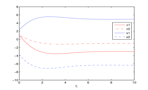
Figure 1: Solution of $(\bar{x},s)$ in Example 5

IV-A1 Comparison

We compare with a fixed point method, which is used to analyze the SCE equation system by verifying a contraction condition in [15]. Consider (10). By the method in [15, 24], the solution $\tilde{x}(t)$ is a fixed point to the equation $x(\cdot)=\Psi(x(\cdot))$ where

$$[\Psi(x)](t)=e^{\mathcal{A}t}x_{0}+\int_{0}^{t}e^{\mathcal{A}(t-s)}BR^{-1}B^{T}$$

$$\qquad\qquad\qquad\cdot\left[\int_{s}^{\infty}e^{-\mathcal{A}^{T}(s-\tau)}\left(Q_{\Gamma}x(\tau)+e^{-\frac{\rho}{2}\tau}\eta_{\Gamma}\right)d\tau\right]ds,$$

where we look for $x(\cdot)\in C_{b}([0,\infty),\mathbb{R}^{n})$, i.e., the set of bounded and continuous functions on $[0,\infty)$ with norm $|x|_{\infty}=\sup_{t\geq 0}|x(t)|$. The fixed point exists and is unique if there exists $\beta\in(0,1)$ such that $|\Psi(x)-\Psi(y)|_{\infty}\leq\beta|x-y|_{\infty}.$ Let $\|\cdot\|$ denote the Frobenius norm. We have the estimate

$$\|[\Psi(x)](t)-[\Psi(y)](t)\|$$

$$=\|\int_{0}^{t}e^{\mathcal{A}(t-s)}BR^{-1}B^{T}$$

$$\qquad\qquad\cdot\left\{\int_{s}^{\infty}e^{-\mathcal{A}^{T}(s-\tau)}\left[Q_{\Gamma}\left(x(\tau)-y(\tau)\right)\right]d\tau\right\}ds\|$$

$$\leq\left\|x-y\right\|\int_{0}^{\infty}\|e^{\mathcal{A}s}BR^{-1}B^{T}\|\left(\int_{0}^{\infty}\|e^{\mathcal{A}^{T}\tau}Q_{\Gamma}\|d\tau\right)ds.$$

Let $\beta=\int_{0}^{\infty}\left\|e^{\mathcal{A}s}BR^{-1}B^{T}\right\|(\int_{0}^{\infty}\|e^{\mathcal{A}^{T}\tau}Q_{\Gamma}\|d\tau)ds$. We note that the upper bound estimate may not be tight.

For Example 5 with $\gamma=2$, we numerically obtain $\beta=6.34694>1$, which does not validate the contraction condition. If we set $\gamma=0.05$ instead, then $\beta=0.736681<1$ implying the contraction condition.

IV-B The Mean Field Game

The next example uses the Schur decomposition for a general square real matrix.

Example 6

Consider $A=\begin{bmatrix}5&-5\\ 0&10\end{bmatrix},\ B=\begin{bmatrix}1\\ 1\end{bmatrix},\ Q=\begin{bmatrix}1&0\\ 0&1\end{bmatrix},\ \eta=\begin{bmatrix}1\\ 0\end{bmatrix},\$ $\Gamma=\begin{bmatrix}5&0\\ 2.5&5\end{bmatrix}$, $\rho=2$, $R=1$, and the initial condition is $x_{0}=\begin{bmatrix}1\\ 1\end{bmatrix}.$ By (23), we calculate

$$M_{\rm mfg}=\begin{bmatrix}14.7999&-42.0915&-1.0000&-1.0000\\ 10.7999&-28.0915&-1.0000&-1.0000\\ 5.0000&0&-14.7999&-10.7999\\ 2.5000&5.0000&42.0915&28.0915\end{bmatrix},$$

which has eigenvalues $9.2522$, $1.7783$, $-2.0950$ and $-8.9356$. The Schur decomposition represents $M_{\rm mfg}$ as

$$U\begin{bmatrix}-8.9356&-13.4806&27.2557&-35.7593\\ 0&-2.0950&-46.5898&-32.5048\\ 0&0&9.2522&-15.8{}037\\ 0&0&0&1.7783\end{bmatrix}U^{-1},$$

where

$$U=\begin{bmatrix}-0.5425&-0.6081&-0.0928&0.5721\\ -0.3060&-0.4284&-0.3027&-0.7945\\ 0.5543&-0.1947&-0.7863&0.1911\\ -0.5521&0.6394&-0.5305&0.0700\end{bmatrix}.$$

For $U_{11}=\begin{bmatrix}-0.5425&-0.6081\\ -0.3060&-0.4284\end{bmatrix}$, $\det(U_{11})=0.0464>0$, so $U_{11}$ is invertible. We select the initial condition

$$s_{0} =U_{21}U_{11}^{-1}x_{0}+(U_{21}U_{11}^{-1}U_{12}-U_{22})\int_{0}^{\infty}e^{-M_{22}\tau}V_{22}Q\eta e^{-\frac{\rho\tau}{2}}d\tau$$

$$=\begin{bmatrix}2.31075\\ -4.11538\end{bmatrix}.$$

Fig. 2 shows the solution $(\bar{x},s)$ for (19)-(20).

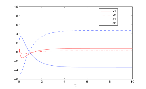
Figure 2: Solution of $(\bar{x},s)$ in Example 6

V Conclusion

This paper develops a methodology to prove the existence and uniqueness of the solution of the LQ social optimization problem when the corresponding Hamiltonian matrix has no eigenvalues on the imaginary axis. We also develop a numerical method for solving the ODE system by applying an invariant subspace method. We further extend the invariant subspace method to solve LQ mean field games.

References

• [1] G. Albi, Y.-P. Choi, M. Fornasier, and D. Kalise. Mean field control hierarchy. Applied Math Optim., vol. 76, no. 1, pp. 93-135, 2017.
• [2] J. Arabneydi and A. Mahajan. Team-optimal solution of finite number of mean-field coupled LQG subsystems. Proc. 54th IEEE CDC, Osaka, Japan, pp. 5308-5313, Dec 2015.
• [3] M. Bardi. Explicit solutions of some linear-quadratic mean field games. Netw. Heterogeneous Media, vol. 7, no. 2, pp. 243-261, 2012.
• [4] A. Bensoussan, J. Frehse, and P. Yam. Mean Field Games and Mean Field Type Control Theory. Springer, New York, 2013.
• [5] A. Bensoussan, K.C.J. Sung, S.C.P. Yam, and S.P. Yung. Linear-quadratic mean-field games. J. Optim. Theory Appl. vol. 169, no. 2, pp. 496-529, 2016.
• [6] D. A. Bini, B. Iannazzo, and B. Meini. Numerical Solution of Algebraic Riccati Equations, Philadelphia: SIAM, 2011.
• [7] P.E. Caines, M. Huang, and R.P. Malhame. Mean Field Games, In Handbook of Dynamic Game Theory, T. Basar and G. Zaccour Eds., Springer, Berlin, 2017.
• [8] X. Chen. Cooperative Linear-Quadratic Mean Field Control and Hamiltonian Matrix Analysis, M.Sc. thesis, Carleton University, Ottawa, Canada, May 2017. Available online at https://curve.carleton.ca/.
• [9] X. Chen and M. Huang. Cooperative linear-quadratic mean field control and its Hamiltonian matrix analysis, arXiv:1801.02306, Jan. 2018.
• [10] K. Du. Solvability conditions for indefinite linear quadratic optimal stochastic control problems and associated stochastic Riccati equations, SIAM J. Control Optim., vol. 53, no. 6, pp. 3673-3689, 2015.
• [11] N. Gast, B. Gaujal, and J.-Y. Le Boudec. Mean field for Markov decision processes: From discrete to continuous optimization. IEEE Trans. Autom. Control, vol. 57, no. 9, pp. 2266-2280, 2012.
• [12] O. Guéant, J.-M. Lasry, and P.-L. Lions. Mean field games and applications. In Paris-Princeton Lectures on Mathematical Finance, pp. 205–266, Springer-Verlag: Heidelberg, Germany, 2011.
• [13] M. Huang, P. E. Caines, and R. P. Malhamé. Individual and mass behaviour in large population stochastic wireless power control problems: centralized and Nash equilibrium solutions. Proc. 42nd IEEE CDC, Maui, HI, pp. 98-103, Dec 2003.
• [14] M. Huang, P. E. Caines, and R. P. Malhamé. Large-population cost-coupled LQG problems with nonuniform agents: Individual-mass behavior and decentralized Nash equilibria. IEEE Transactions on Automatic Control, vol. 52, no. 9, pp. 1560-1571, 2007.
• [15] M. Huang, P. E. Caines, and R. P. Malhamé. Social optima in mean field LQG control: Centralized and decentralized strategies. IEEE Trans. Autom. Control, vol. 57, no. 7, pp. 1736-1751, 2012.
• [16] M. Huang, R. P. Malhamé, and P. E. Caines. Large population stochastic dynamic games: closed-loop McKean-Vlasov systems and the Nash certainty equivalence principle. Commun. Inform. Systems, vol. 6, no. 3, pp. 221-252, 2006.
• [17] M. Huang and S. L. Nguyen. Linear-quadratic mean field teams with a major agent. Proc. 55th IEEE CDC, Las Vegas, NV, pp. 6958-6963, Dec 2016.
• [18] P. Lancaster and L. Rodman. Algebraic Riccati Equations. Oxford: Clarendon Press, 1995.
• [19] J.-M. Lasry and P.-L. Lions. Mean field games. Japan. J. Math., vol. 2, no. 1, pp. 229-260, 2007.
• [20] A. Laub. A Schur method for solving algebraic Riccati equations. IEEE Trans. Automatic Control, vol. 24, no. 6, pp. 913-921, 1979.
• [21] T. Li and J.-F. Zhang. Asymptotically optimal decentralized control for large population stochastic multiagent systems. IEEE Trans. Automat. Control, vol. 53, pp. 1643-1660, 2008.
• [22] C. Van Loan. A symplectic method for approximating all the eigenvalues of a Hamiltonian matrix. Linear Algebra and its Applications, vol. 61, pp. 233-251, 1984.
• [23] J. Moon and T. Basar. Linear quadratic risk-sensitive and robust mean field games. IEEE Trans. Autom. Control, vol. 62, no. 3, pp. 1062-1077, 2017.
• [24] M. Nourian, P. E. Caines, R. P. Malhamé, and M. Huang. Mean field LQG control in leader-follower stochastic multi-agent systems: Likelihood ratio based adaptation. IEEE Trans. Autom. Control, vol. 57, no. 11, pp. 2801-2816, 2012.
• [25] M. Nourian, P. E. Caines, R.P. Malhamé and M. Huang. Nash, social and centralized solutions to consensus problems via mean field control theory. IEEE Trans. Autom. Control, vol. 58, pp. 639-653, Mar 2013.
• [26] G. Nuno and B. Moll. Social optima in economies with heterogeneous agents. Review of Economic Dynamics, 2017, available online.
• [27] T. Pappas, A. Laub, and N. Sandell. On the numerical solution of the discrete-time algebraic Riccati equation. IEEE Trans. on Automatic Control, vol. 25, no. 4, pp. 631-641, 1980.
• [28] B. Piccoli, F. Rossi, and E. Trelat. Control to flocking of the kinetic Cucker-Smale model. SIAM J. Math. Anal., vol. 47, no. 6, pp. 4685-4719, 2015.
• [29] M.A. Rami, and X. Y. Zhou. Linear matrix inequalities, Riccati equations, and indefinite stochastic linear quadratic controls, IEEE Trans. Autom. Control, vol. 45, no. 6, pp. 1131-1143, 2000.
• [30] N. Sen, M. Huang, and R. P. Malhame. Mean field social control with decentralized strategies and optimality characterization. Proc. 55th IEEE CDC, Las Vegas, NV, pp. 6056-6061, Dec 2016.
• [31] B.-C. Wang and J.-F. Zhang. Social optima in mean field linear-quadratic-Gaussian models with Markov jump parameters. SIAM J. Control Optim., vol. 55, no. 1, pp. 429-456, 2017.
• [32] J. Willems. Least squares stationary optimal control and the algebraic Riccati equation. IEEE Trans. Automatic Control, vol. 16, no. 6, pp. 621-634, 1971.
• [33] W. M. Wonham. Linear Multivariable Control: A Geometric Approach. Springer, New York, NY, 3rd edition, 2012.
• [34] D.W.K. Yeung and L. A. Petrosyan. Cooperative Stochastic Differential Games, Springer, New York, 2006.
• [35] K. Zhou, J.C. Doyle and K. Glover. Robust and Optimal Control, Upper Saddle River, N.J.: Prentice Hall, 1996.
• [36] J. Yong and X.Y. Zhou, Stochastic Controls: Hamiltonian Systems and HJB Equations, Springer, New York, 1999.