Adversarial Perturbation Intensity Achieving Chosen Intra-Technique Transferability Level for Logistic Regression

Abstract

Machine Learning models have been shown to be vulnerable to adversarial examples, ie. the manipulation of data by a attacker to defeat a defender’s classifier at test time. We present a novel probabilistic definition of adversarial examples in perfect or limited knowledge setting using prior probability distributions on the defender’s classifier. Using the asymptotic properties of the logistic regression, we derive a closed-form expression of the intensity of any adversarial perturbation, in order to achieve a given expected misclassification rate. This technique is relevant in a threat model of known model specifications and unknown training data. To our knowledge, this is the first method that allows an attacker to directly choose the probability of attack success. We evaluate our approach on two real-world datasets.

1 Introduction

Adversarial examples theory is the study of the strategies of a defender and an attacker in the following threat model: an adversary has the ability of modifying an input, noted $x_{0}$ here, with the goal of crafting a new input $x_{adv}$ that will be misclassified by the defender’s classification model. The perturbation is noted $\delta_{0}$. Note that the attack happens at test time. The attacker doesn’t have the ability to alter the integrity of the model estimation.

$$x_{adv}=x_{0}+\delta_{0}$$

With $k$ known, untargeted adversarial examples crafting is usually defined by the following optimization problem:

$$\delta_{0}=\arg\min_{\delta}\lVert\delta\rVert_{k}\;\quad\text{s.t.}\quad f_{d}(x_{0}+\delta;\hat{\theta}_{d})\neq y_{0}$$

where $f_{d}\colon\mathcal{X}\times\Theta\to\mathcal{Y},\quad x\times\theta\mapsto y$ is the classifier (or prediction function) of the defender’s model, $\hat{\theta}_{d}$ is the defender’s estimate of the model parameters, $\mathcal{X}$ the input space, $\mathcal{Y}$ the output space, and $\Theta$ the parameters space. Note that some authors prefer another definition for adversarial examples (Biggio & Roli, 2017).

Some authors define the optimization problem by using $f_{d}(x_{0};\hat{\theta}_{d})$ instead of $y_{0}$. We prefer to use $y_{0}$, because if the original input is already misclassified by the model, ie. $f_{d}(x_{0};\hat{\theta}_{d})\neq y_{0}$, then $\delta_{0}=0_{p}$, with $p$ the number of features, if $f_{d}$ and $\hat{\theta}_{d}$ are known. This point has consequences in limited knowledge settings developed in part 4.

To this definition, the attacker may add application specific constraints on $\delta$. Various have been used in the literature:

• $x_{0}+\delta\in\mathcal{X}$, where $\mathcal{X}$ may be $\mathbb{N}$

• $\lVert\delta\rVert_{k}<d_{\text{max}}$ (Biggio et al., 2013)

• $\forall i,\delta_{i}\geq 0$ (Grosse et al., 2017)

Similar conditions can be derived only on a subset of features. For simplicity reasons, we will not use any of these conditions in the following. We assume that $\mathcal{X}=\mathbb{R}^{p}$.

The attacker doesn’t necessary have the same knowledge than the defender. Knowing the defender’s training data and model specifications, the attacker can train an exact copy of $f_{d}(\cdot,\hat{\theta}_{d})$. With partial knowledge of $f_{d}(\cdot,\hat{\theta}_{d})$, the attacker can train a substitute model to craft adversarial examples from it (Biggio et al., 2013; Papernot et al., 2016a, 2017). Papernot et al. (2016b) build a typology of attacks depending on the knowledge that the attacker have on the defender’s model and on the goal of the attacker. Biggio et al. (2013) detail the components of the attacker’s knowledge:

• the defender’s training data (completely or only a subset)

• feature representation used by the defender

• the type of learning algorithm and the decision function, that we called model specification

• the defender’s estimate of the model parameters.

The capability of the adversary may provide extra knowledge on the defender’s model. The typical example is the case of the attacker having feedback from the defender’s model (Papernot et al., 2017).

The property of transferability of adversarial examples, defined by the fact that some adversarial examples designed to fool a specific model also fool other models, was observed by Goodfellow, Shlens, and Szegedy (2014), Papernot et al. (2016a), Papernot et al. (2017), among others. Papernot et al. (2016a) identify two types of transferability: intra-technique transferability and cross-technique transferability.

The optimal L2-adversarial example for a logistic regression (with perfect knowledge) is the orthogonal projection of the example onto the decision hyperplane (Moosavi-Dezfooli et al., 2016). In part 4, we use this technique to compute adversarial example, but our method can be applied to any adversarial example crafting technique.

The intuition guiding our work our work is that an optimal adversarial example for the attacker surrogate model, given the limited knowledge of the attacker, may not achieve satisfactory intra-technique transferability. If the adversarial example is very close to the decision hyperplane, a very small difference between $\hat{\theta}_{d}$ and $\hat{\theta}_{a}$ can lead to failed attacks.

In part 2, we provide a probabilistic definition of an adversarial example. In part 3, we recall the asymptotic properties of the logistic regression. In part 4, we develop a closed-form approximate of an adversarial example having a chosen expected successful attack rate, in the threat model of known model specification but unknown training data for binary classification by a logistic regression. In part 5, we apply our method on 2 datasets.

Contributions

• We introduce a new probability-based definition of adversarial example having an arbitrary expected misclassification rate using prior distributions to formalize the attacker knowledge on the defender’s classifier.

• We make use of the asymptotic distribution of logistic regression parameters to derive a closed form method to craft adversarial examples having a chosen expected success attack rate, in a limited knowledge threat model. To our knowledge, this is the first method to allow an attacker to directly tune the probability of attack success.

• We show that multiplying by the same scalar all adversarial perturbations of the test samples computed on the attacker’s surrogate model may not be effective to improve intra-technique transferability.

• We observe the importance of knowing the estimation method used by the defender, even for logistic regression.

• We notice that in our setting the choice of the L2-regularization hyperparameter can be beneficial to the attacker by reducing the variance of parameters estimates.

2 Probabilistic definition of adversarial example ($\alpha$-adversarial example)

We define an $\alpha$-adversarial example as an adversarial example with an expected rate of successful attacks of $\alpha$ in an perfect or imperfect knowledge setting:

$$\min_{\delta}\lVert\delta\rVert_{k}\quad\text{s.t.}\\ \mathbb{P}\left(F_{d}(x_{0}+\delta;\hat{\theta}_{d})\neq y_{0}\Big{|}F_{d}\sim\mathscr{D}_{F_{d}}\cap\hat{\theta}_{d}\sim\mathscr{D}_{\hat{\theta}_{d}}(F_{d})\right)\geq\alpha$$ (1)

where $\alpha\in[0,1]$ is chosen by the attacker.

$F_{d}$ is a random function drawn from the sample space $\mathcal{F}\subset\mathcal{Y}^{\mathcal{X}}$ of the set of prediction functions that the defender can use. $\mathscr{D}_{F_{d}}$ is the prior knowledge of the attacker on feature representation, model type, its structural specifications (for example, the architecture of a Neural Network), used by the defender. We consider $\mathcal{X}$ as the space of raw data, and we include the data preprocessing step into $F_{d}$. $\mathscr{D}_{\hat{\theta}_{d}}(F_{d})$ captures the prior knowledge on the defender’s estimates of parameters, training data, estimation methods, regularization, hyperparameters of the model and of the feature representation. Then, $\mathscr{D}_{\hat{\theta}_{d}}(F_{d})$ is the joined prior and hyperprior of the parameters of $F_{d}$. The Data Generating Process (DGP) $\mathcal{P}_{\theta}(X,Y)$ is parametrized by $\theta$, the vector of true model parameters and hyperparameters, and of feature representation hyperparameters. The distribution of $\hat{\theta}_{d}$ is conditioned by $F_{d}$, because the model (hyper)parameters may vary across model types.

We formalize the knowledge of the attacker using the joined probability distribution of $F_{d}$ and $\hat{\theta}_{d}$. If the attacker knows perfectly the true defender’s decision function $f_{d}$, then $\mathscr{D}_{F_{d}}$ is a deterministic distribution and $\forall f\in\mathcal{F},\ \mathbb{P}\left(F_{d}=f\right)=1_{f_{d}}(f)$. Instead the attacker may have only partial knowledge on the attacker model. In practice, the attacker may know the state-of-the-art models or the industry practices on a given task. Then, the adversary may be able to draw a probability distribution on a set of models used by the defender. The attacker may also draw probability distributions of hyperparameters depending on the method used by the defender (random search, grid search, etc.).

The attacker might want to estimate $\mathscr{D}_{F_{d}}$ using $\hat{f}_{a}$ his/her estimate of $f_{d}$ and estimate $\mathscr{D}_{\hat{\theta}_{d}}(F_{d})$ using $(\hat{f}_{a},\hat{\theta}_{a})$. This remark makes particularly sense if the attacker has an oracle access to the defender model.

3 Recalls of the asymptotic properties of the logistic regression

The logistic regression can be seen as a Generalized Linear Model (GLM) with Binomial distribution and a logit link.

A GLM is defined by 3 components (Fox, 2016, p. 379):

1. A conditional distribution of the response variable $Y_{i}$ given $X_{i}$, member of the exponential family distribution. $Y_{i}$ are independent.

2. A linear predictor, $\eta_{i}=\beta_{0}+\beta_{1}X_{i,1}+\beta_{2}X_{i,2}+\cdots+\beta_{p}X_{i,p}$.

3. A smooth and invertible link function $g(\cdot)$, $\eta_{i}=g(\mu_{i})$.

Note that the point 1. implies that a GLM is not only a transformation of the classical linear model using a link function. GLM doesn’t have the hypothesis of normality of the residuals.

Then, the logistic regression is a special case of GLM with $Y_{i}\sim\mathcal{B}(m_{i},\pi_{i})$ and the logit function as link (which is the canonical link of the Binomial distribution). Note that $m_{i}$ is known, so it isn’t a parameter of the model.

The Maximum Likelihood Estimator $\hat{\beta}_{\text{MLE}}$ is asymptotically normally distributed (Ferguson, 1996, p. 121). It is asymptotically unbiased with an asymptotic variance-covariance matrix equals to the inverse of the Fisher information matrix

$$\left(X^{\intercal}WX\right)^{-1},$$

with $W$ a diagonal matrix of weights defined by $W:=\text{diag}\left\{m_{i}\pi_{i}(1-\pi_{i})\right\}$ (McCullagh & Nelder, 1989, p. 119). $W$ can be estimated by $\widehat{W}=\text{diag}\left\{m_{i}\hat{\pi}_{i}(1-\hat{\pi}_{i})\right\}$. Note that the same asymptotic property holds when $n$ is fixed and $m\to\infty$.

The ridge estimator in logistic regression, noted $\hat{\beta}_{\text{L2},\lambda_{\text{L2}}}$, is a maximum a posteriori (MAP) estimator. Therefore it is asymptotically normal (Ferguson, 1996, p. 140), asymptotically biased and the asymptotic variance-covariance matrix is given by (Le Cessie & van Houwelingen, 1992):

$$\left(X^{\intercal}WX+2\lambda_{\text{L2}}I_{p}\right)^{-1}X^{\intercal}WX\left(X^{\intercal}WX+2\lambda_{\text{L2}}I_{p}\right)^{-1}$$

Then, if $n$ is large, we can use the following approximations to estimate the variance-covariance matrices:

$$\begin{split}\widehat{\mathrm{Var}}\left(\hat{\beta}_{\text{MLE}}\right)=&\left(X^{\intercal}\widehat{W}X\right)^{-1}\\ \widehat{\mathrm{Var}}\left(\hat{\beta}_{\text{L2},\lambda_{\text{L2}}}\right)=&\left(X^{\intercal}\widehat{W}X+2\lambda_{\text{L2}}I_{p}\right)^{-1}X^{\intercal}\widehat{W}X\\ &\left(X^{\intercal}\widehat{W}X+2\lambda_{\text{L2}}I_{p}\right)^{-1}\end{split}$$

4 Approximation of $\alpha$-adversarial examples for the logistic regression

For convenience, in this section we define $\tilde{x}_{0}:=~{}\begin{pmatrix}1\\ x_{0}\end{pmatrix}~{}\in~{}\mathbb{R}^{p+1}$ and $\tilde{\delta}_{0}:=\begin{pmatrix}0\\ \delta_{0}\end{pmatrix}\in\mathbb{R}^{p+1}$.

We will consider the following threat model:

Perfect knowledge of $f_{d}$

• The defender is using a logistic regression to perform a binary classification task,

  $$\forall(x_{0},\beta)\in\mathbb{R}^{p}\times\mathbb{R}^{p+1},\ f_{d}(x_{0},\beta)=\begin{cases}1&\text{if }\tilde{x}_{0}^{\intercal}\beta>0,\\ 0&\text{otherwise}.\end{cases}$$

• The attacker knows perfectly the defender’s feature representation.

Limited knowledge of $\hat{\theta}_{d}$

• The attacker doesn’t have access to the defender’s training data.

• The attacker has access to some surrogate training data generated by the same Data Generating Process (DGP) parametrized by $\beta\in\mathbb{R}^{p+1}$.

• The attacker knows the specifications of the logistic regression (regularization method and hyperparameters, estimation method).

Therefore the defender’s parameters estimation $\hat{\beta}_{d}$ is fixed but unknown by the attacker. The attacker can compute $\hat{\beta}_{a}$ using his/her own data.

The goal of the attacker is to find $\delta^{*}$ solving problem 2.

$$\delta^{*}=\arg\min_{\delta\in\mathbb{R}^{p}}\lVert\delta\rVert_{k}\;\quad\text{s.t.}\quad\mathbb{P}\left[f_{d}(x_{0}+\delta;\hat{\beta}_{d})\neq y_{0}\right]\geq\alpha$$ (2)

where $k\in\{1,2\}$ and $\alpha\in[0,1]$ are chosen by the attacker.

For simplicity purposes, we consider the following suboptimal problem.

First step: The attacker compute an adversarial example for his/her own model. Any adversarial example crafting technique can be used.

$$\delta_{0}=\arg\min_{\delta\in\mathbb{R}^{p}}\lVert\delta\rVert_{k}\;\quad\text{s.t.}\quad f_{d}(x_{0}+\delta;\hat{\beta}_{a})\neq y_{0}$$

In the following, we consider the L2-optimal adversarial example ($k=2$) which is the orthogonal projection of $x_{0}$ on the decision hyperplane $\mathcal{H}_{a}=\{x\in\mathbb{R}^{p}\;|\;f_{d}(x;\hat{\beta}_{a})=0\}$ (Moosavi-Dezfooli et al., 2016). The associated perturbation can be computed by

$$\delta_{0}=-\frac{\tilde{x}_{0}^{\intercal}\hat{\beta}_{a}}{\lVert\hat{\beta}_{\text{a;-0}}\rVert^{2}_{2}}\hat{\beta}_{\text{a;-0}}$$

where $\hat{\beta}_{\text{a;-0}}=\left(\hat{\beta}_{a;1},\hat{\beta}_{a;2},\cdots,\hat{\beta}_{a;p}\right)^{\intercal}$.

Second step: The attacker searches an optimal scalar $\lambda^{*}$, the intensity of the adversarial perturbation $\delta_{0}$, needed to achieve an expected misclassification rate on the defender’s model of at least $\alpha$:

$$\lambda^{*}=\arg\min_{\lambda\in\mathbb{R}}\lVert\lambda\delta_{0}\rVert_{k^{\prime}}\;\ \text{s.t.}\ \mathbb{P}\left[f_{d}(x_{0}+\lambda\delta_{0};\hat{\beta}_{d})\neq y_{0}\right]\geq\alpha$$

with $k^{\prime}\in\{1,2\}$. It can be simplified as

$$\lambda^{*}=\arg\min_{\lambda\in\mathbb{R}}\lambda^{2}\;\quad\text{s.t.}\quad\mathbb{P}\left[f_{d}(x_{0}+\lambda\delta_{0};\hat{\beta}_{d})\neq y_{0}\right]\geq\alpha$$ (3)

We denote the $\alpha$-adversarial example: $x_{adv}^{*}:=x_{0}+\lambda^{*}\delta_{0}$.

Problem 3 can be rewritten as

$$\min_{\lambda\in\mathbb{R}}g(\lambda)\enspace\text{s.t.}\enspace h(\lambda)\geq 0$$

with $g\colon\mathbb{R}\to\mathbb{R}^{+},\quad\lambda\mapsto\lambda^{2}$ and $h\colon\mathbb{R}\to[-1,1],\quad$ $\lambda\mapsto\mathbb{P}\left[f_{d}(x_{0}+\lambda\delta_{0};\hat{\beta}_{d})\neq y_{0}\right]-\alpha$.

$g$ and $h$ are of class $C^{1}$. Then using the complementary slackness of the Karush–Kuhn–Tucker conditions, if $\lambda^{*}$ is a local optimum, $h(\lambda^{*})g^{\prime}(\lambda^{*})=0$ . If $h(\lambda^{*})=0$ the constraint is said to be saturated, and if $g^{\prime}(\lambda^{*})=0$ it is not saturated.

4.1 Case 1: Constraint saturated, ie. $\mathbb{P}\left[f_{d}(x_{0}+\lambda\delta_{0};\hat{\beta}_{d})\neq y_{0}\right]=\alpha$

For convenience, we define the random variable $Z$ as follow:

$$\forall\lambda\in\mathbb{R},\quad Z:=(\tilde{x}_{0}+\lambda\tilde{\delta}_{0})^{\intercal}\hat{\beta}_{d}$$

For large samples, $\hat{\beta}_{d}\rightsquigarrow\mathcal{N}\left(\mathbb{E}(\hat{\beta}_{d}),\mathrm{Var}(\hat{\beta}_{d})\right)$.

Then, $Z\rightsquigarrow\mathcal{N}\left(\mathbb{E}(Z),\mathrm{Var}(Z)\right)$ with

$$\mathbb{E}(Z) =(\tilde{x}_{0}+\lambda\tilde{\delta}_{0})^{\intercal}\mathbb{E}(\hat{\beta}_{d}),$$

$$\mathrm{Var}(Z) =(\tilde{x}_{0}+\lambda\tilde{\delta}_{0})^{\intercal}\mathrm{Var}(\hat{\beta}_{d})(\tilde{x}_{0}+\lambda\tilde{\delta}_{0}).$$

The attacker estimates $\mathbb{E}(\hat{\beta}_{d})$ by $\hat{\beta}_{a}$, and $\mathrm{Var}(\hat{\beta}_{d})$ by $\widehat{\mathrm{Var}}(\hat{\beta}_{a})$ which is computed as explained in part 3.

4.1.1 Subcase a: $y_{0}=1$

Using the quantile function of the normal distribution, if $y_{0}=1$:

$$\mathbb{P}\left[f_{d}(x_{0}+\lambda\delta_{0};\hat{\beta}_{d})\neq y_{0}\right]=\alpha$$

$$\Leftrightarrow\mathbb{P}\left(Z\leq 0\right)=\alpha$$

$$\Leftrightarrow(\tilde{x}_{0}+\lambda\tilde{\delta}_{0})^{\intercal}\hat{\beta}_{d}$$

$$\quad+\sqrt{(\tilde{x}_{0}+\lambda\tilde{\delta}_{0})^{\intercal}\mathrm{Var}(\hat{\beta}_{d})(\tilde{x}_{0}+\lambda\tilde{\delta}_{0})}\sqrt{2}\operatorname{erf}^{-1}(2\alpha-1)$$

$$\quad=0$$ (4)

Equation 4 is estimated by the attacker by :

$$(\tilde{x}_{0}+\lambda\tilde{\delta}_{0})^{\intercal}\hat{\beta}_{a}$$

$$\quad+\sqrt{(\tilde{x}_{0}+\lambda\tilde{\delta}_{0})^{\intercal}\widehat{\mathrm{Var}}(\hat{\beta}_{a})(\tilde{x}_{0}+\lambda\tilde{\delta}_{0})}\sqrt{2}\operatorname{erf}^{-1}(2\alpha-1)$$

$$\quad=0$$

$$\Rightarrow\left[(\tilde{x}_{0}+\lambda\tilde{\delta}_{0})^{\intercal}\hat{\beta}_{a}\right]^{2}$$

$$\quad-(\tilde{x}_{0}+\lambda\tilde{\delta}_{0})^{\intercal}\widehat{\mathrm{Var}}(\hat{\beta}_{a})(\tilde{x}_{0}+\lambda\tilde{\delta}_{0})2\left[\operatorname{erf}^{-1}(2\alpha-1)\right]^{2}$$

$$\quad=0$$

$$\Rightarrow(\tilde{x}_{0}+\lambda\tilde{\delta}_{0})^{\intercal}\hat{\beta}_{a}\hat{\beta}_{a}^{\intercal}(\tilde{x}_{0}+\lambda\tilde{\delta}_{0})$$

$$\quad-(\tilde{x}_{0}+\lambda\tilde{\delta}_{0})^{\intercal}\widehat{\mathrm{Var}}(\hat{\beta}_{a})(\tilde{x}_{0}+\lambda\tilde{\delta}_{0})2\left[\operatorname{erf}^{-1}(2\alpha-1)\right]^{2}$$

$$\quad=0$$

$$\Rightarrow(\tilde{x}_{0}+\lambda\tilde{\delta}_{0})^{\intercal}\left[\hat{\beta}_{a}\hat{\beta}_{a}^{\intercal}-2\left(\operatorname{erf}^{-1}(2\alpha-1)\right)^{2}\widehat{\mathrm{Var}}(\hat{\beta}_{a})\right]$$

$$\quad(\tilde{x}_{0}+\lambda\tilde{\delta}_{0})=0$$

$$\Rightarrow\tilde{x}_{0}^{\intercal}A\tilde{x}_{0}+\lambda(\tilde{x}_{0}^{\intercal}A\tilde{\delta}_{0}+\tilde{\delta}_{0}^{\intercal}A\tilde{x}_{0})+\lambda^{2}\tilde{\delta}_{0}^{\intercal}A\tilde{\delta}_{0}=0$$

with $A:=\hat{\beta}_{a}\hat{\beta}_{a}^{\intercal}-2\left(\operatorname{erf}^{-1}(2\alpha-1)\right)^{2}\widehat{\mathrm{Var}}(\hat{\beta}_{a})$.

Then, $\lambda\in\mathbb{R}$ can be computed by solving a second degree equation. If there are two solutions, we choose the one that satisfy Equation 4. We denote the solution of the second degree equation $\lambda_{\alpha}$.

4.1.2 Subcase b: $y_{0}=0$

$$\mathbb{P}\left[f_{d}(x_{0}+\lambda\delta_{0};\hat{\beta}_{d})\neq y_{0}\right]=\alpha$$

$$\Leftrightarrow\mathbb{P}\left(Z\leq 0\right)=1-\alpha$$

$\lambda_{\alpha}$ can be derived similarly to subcase a, replacing $\alpha$ by $1-\alpha$.

4.2 Case 2: Constraint not saturated, ie. $\mathbb{P}\left[f_{d}(x_{0}+\lambda\delta_{0};\hat{\beta}_{d})\neq y_{0}\right]>\alpha$

In this case, $g^{\prime}(\lambda^{*})=0$. It immediately follows that $\lambda^{*}=0$.

If $\mathbb{P}\left[f_{d}(x_{0};\hat{\beta}_{d})\neq y_{0}\right]>\alpha$, then 0 is the global minimum. Otherwise and if $\lambda_{\alpha}$ exists, then $\lambda_{\alpha}$ is the global minimum, because it is the unique point that saturates the constraint.

To sum up, the problem 3 can be solved by:

$$\lambda^{*}=\begin{cases}0&\text{if }\mathbb{P}\left[f_{d}(x_{0};\hat{\beta}_{d})\neq y_{0}\right]>\alpha,\\ \lambda_{\alpha}&\text{otherwise}.\end{cases}$$

5 Applications

We applied our analysis on 2 datasets: the UCI spambase set and the dogs vs cats image set. These two datasets are binary classification problems. The code is available for reproducibility purpose on GitHub and Framagit.

Table 1: Classification accuracies for the 3 estimation methods studied on the spam dataset.

Estimation method	Accuracy in-sample	Accuracy out-of-sample
IRLS	93.11%	92.61%
Unregularized liblinear	93.11%	92.75%
L2-regularized liblinear	93.14%	92.75%

5.1 Spambase Data Set

The UCI spam dataset is small enough to estimate the logistic regression using the Iteratively Reweighted Least Squares (IRLS) estimation method, generally used for GLM, provided by the statsmodels Python module. We also trained an unregularized and a L2-regularized logistic regression using the Scikit-learn implementation and the liblinear solver.

The accuracies are pretty similar between estimation methods (Table 1). But the estimated variance-covariance matrices are very different from the IRLS estimation and the liblinear ones. It leads to very different intensities to achieve the same misclassification level for some examples. In Table 2, we can observe very different values of $\lambda^{*}$ across the 3 estimation methods studied for a arbitrary example $x_{0}$ in the test set. This is mainly due to the high difference in the estimations of $\beta_{41}$, because $\hat{\beta}_{41;\text{IRLS}}=-48.08$, $\hat{\beta}_{41;\text{URLB}}=-3.07$ and $\widehat{\mathrm{Var}}\left(\hat{\beta}_{41;\text{IRLS}}\right)-\widehat{\mathrm{Var}}\left(\hat{\beta}_{41;\text{URLB}}\right)=1332.74$ whereas the second biggest element-wise difference between the two covariance matrices in absolute value is $12.56$. It emphasis the importance of knowing the estimation method used by the defender.

Table 2: Predicted probabilities of being a spam by the attacker model of an arbitrary test examples $x_{0}$, its original perturbation $x_{0}+\delta_{0}$, and its intensified perturbation $x_{0}+\lambda^{*}\delta_{0}$, and values of the intensities $\lambda^{*}$, for the 3 estimation methods studied on the spam dataset. Note that $y_{0}=1$ and $\alpha=0.95$.

Predicted probabilities and Intensities	IRLS	Unregularized liblinear	L2-regularized liblinear
$\mathbb{P}(Y=1|X=x_{0},\hat{\beta}_{a})$	99.999986%	99.999892%	99.999919%
$\mathbb{P}(Y=1|X=x_{0}+\delta_{0},\hat{\beta}_{a})$	49.999606%	49.999656%	49.999649%
$\mathbb{P}(Y=1|X=x_{0}+\lambda^{*}\delta_{0},\hat{\beta}_{a})$	$1.687831e^{-74}\%$	1.004755%	2.040357%
$\lambda^{*}$	12.059536	1.333934	1.275921

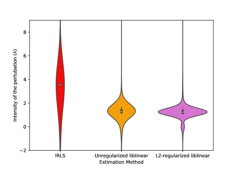
Figure 1: Violin plot of the intensities of perturbations in the test set for $\alpha=0.9$. The figure is zoomed in for better visualization.

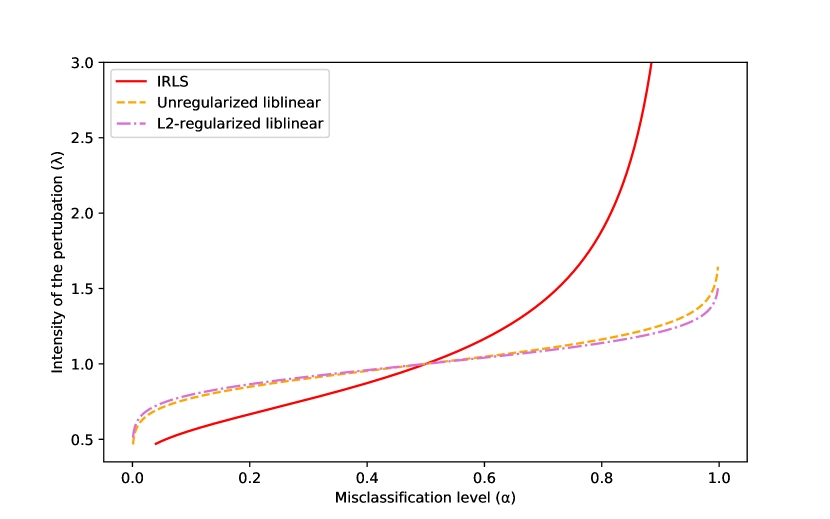
Figure 2: Intensities of perturbations versus misclassification levels for the same example $x_{0}$ than Table 2.

Table 2 also reports the estimated probabilities of being a spam by the attacker model for the intensified perturbations of $x_{0}$ across estimation methods. It insists on the fact that we do not have to confound the estimated probability of an adversarial example to be in a specific class by the attacker’s surrogate model, and the probability $\alpha$ of being classified in a specific class by the defender’s model.

Figure 2 represents the intensity of the adversarial orthogonal perturbation against misclassification levels from 0 to 1 for the same arbitrary example $x_{0}$. The intensity associated to the IRLS estimation is higher than the other two for all values of $\alpha$ higher than 0.5, and it explodes sooner when $\alpha$ tends towards 1. Notice that the the intensities have different scale across examples. It confirm our intuition that multiplying all examples by the same scalar in not the best way to improve intra-technique transferability.

Figure 1 shows the box plots and the kernel density estimations of the perturbation intensity in the test set for a fixed misclassification level of $0.90$ across the estimation methods. The median of intensities computed on the unregularized model is sightly greater than the one on the L2-regularized model.

Figure 3: Quantiles of the empirical distributions of the intensities $\lambda^{*}$ in the test set and out-of-sample accuracy, versus values of the L2-regularization hyperparameter $\lambda_{\text{L2}}$ (in log-scale). The red lower bound represents the first decile, the red upper one the last decile, and the red line the median.

Figure 3 represents the evolution of the intensities of the adversarial perturbations with respect to the L2-regularization hyperparameter. The relation is not straightforward. A very strong regularization is beneficial to the attacker, because it leads to very small parameter variance, which at the end implies smaller perturbations to achieve the same misclassification level. A very small values of regularization leads to instability in the intensities, which is good for the defender. Interestingly, when the regularization is strong enough to lower the accuracy, it increases the intensity until saturation of the constraint ($\lambda^{*}=0$). With this exception in mind, we can globally said that if regularization leads to better estimates in terms of MSE (Mansson & Shukur, 2011), it is also beneficial to the attacker. Then, we make the hypothesis that there is a trade-off in the defender’s choice of L2-regularization hyperparameter between performance and security.

5.2 Dogs vs Cats Images

We also applied our results to the Dogs versus Cats images dataset, available on Kaggle, which is composed of 25000 labeled images of cats and dogs.

We preprocess the images by normalizing the luminance and resizing them to a squared shape of 64 by 64 pixels. The low resolution is necessary for us, because the computation of the variance-covariance matrix needs the inversion of a $p\times p$ matrix. We preserve the aspect ratio by adding gray bars as necessary to make them square. Even using 64 by 64 pixels images, the resulting 12288 features are too large for the GLM estimation using IRLS. We only used the Scikit-learn implementation of logistic regression. We trained a L2-regularized logistic regression, using the SAG solver, where the regularization hyperparameter is chosen by grid search of 100 values on 3-Fold Cross Validation.

Table 3: Classification accuracies the logistic regression trained on the dogs vs cats images.

	Accuracy
In-sample	73.37%
Out-of-sample	58.07%

The accuracy of our model is poor (Table 3), because the data are not linearly separable. It clearly overfits our training data.

We choose to perturb 2 squared images from the test set, which are represented in Figure 5. Original and adversarial images cannot be distinguish by the human eye. Image 1 is correctly classified as a cat. The intensity of the perturbation of this image is a increasing function of the misclassification level (Figure 6(a)): as $\alpha$ increases, the associated adversarial examples is further away from the decision hyperplane. Image 2 is not correctly classified as a cat. Then, the perturbation intensity is negative and is a decreasing function of the misclassification level: a stronger misclassification implies to be further away from the decision boundary in the same half-space where is the original example. As seen in Figure 5(b) and 6(b), the value of $\lambda^{*}$ associated to Image 2 for $\alpha=0.75$ is $0$, because the probability that the original example is misclassified is $0.88$.

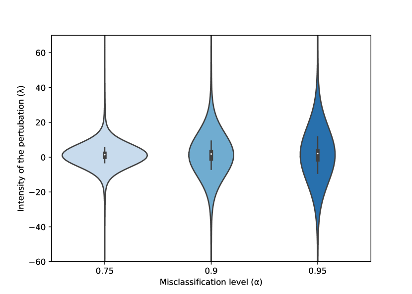
Figure 4: Violin plot of the intensities of perturbations in the test set for different levels of misclassification. The figure is zoomed in for better visualization.

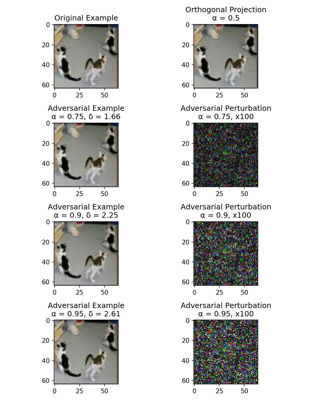
(a) Image 1

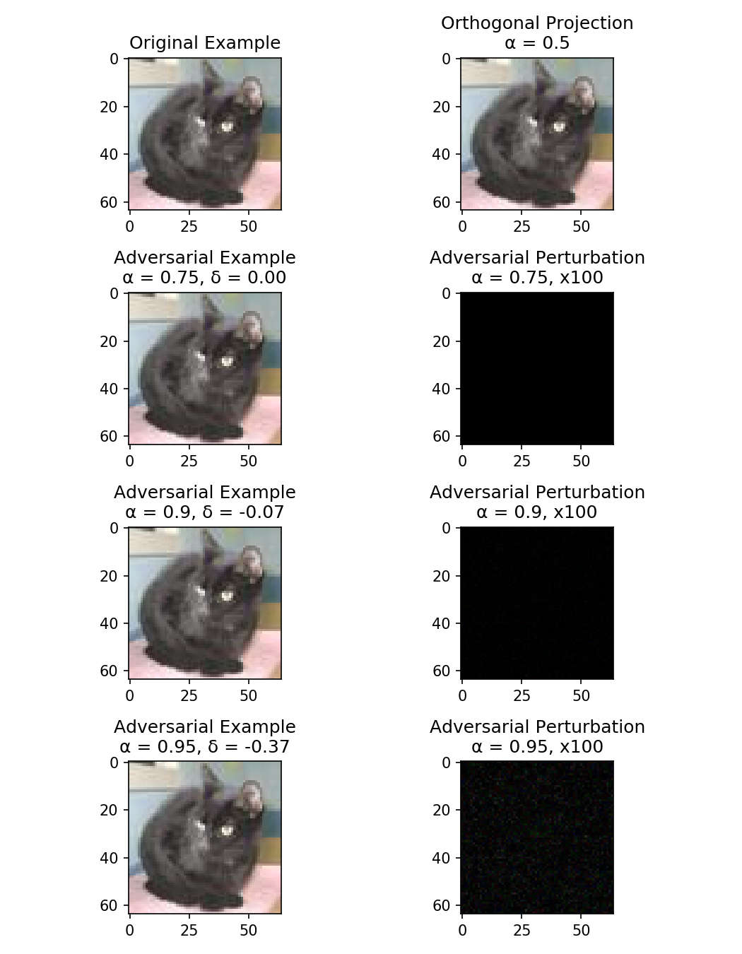
(b) Image 2

Figure 5: Original image, attacker’s L2-optimal adversarial image, adversarial images achieving misclassification levels of 0.75, 0.90 and 0.95, and their associated perturbations, for 2 images from the test set. Image 1 is correctly classified by our logistic regression and Image 2 is not. Perturbations are represented in absolute values and multiplied by 100.

(a) Test Image 1

(b) Test Image 2

Figure 6: Intensities of perturbations versus misclassification levels.

We computed the intensities associated to the misclassification levels of $0.75$, $0.9$ and $0.95$, for each test example. The empirical distributions of $\lambda^{*}$ grouped by $\alpha$ are represented as violin plots in Figure 4. The intensities are scattered, because of the differences in scales of the initial perturbations $\delta_{0}$, and the fact that the variance-covariance matrix of $\beta$ is higher in some directions of $\delta_{0}$ than others. Moreover, increasing the misclassification level seems to lead to higher empirical variance of the intensities.

5.3 Conclusions, limitations and future work

In this paper, we show a simple way to craft an adversarial example that achieves an expected misclassification rate in the case of limited knowledge, in which the attacker knows that the defender uses a logistic regression, but doesn’t know the defender’s training data. We defined an adversarial example having an expected misclassification rate of $\alpha$ by the defender, as an $\alpha$-adversarial example. Using 2 real-world datasets, we show the importance to compute the intensity of adversarial perturbations at the individual level: computing an adversarial perturbation on the attacker surrogate model and applying the same intensity across all perturbations is a suboptimal strategy to achieve satisfactory intra-technique transferability.

Our method can be used on any adversarial perturbation technique that only uses the surrogate attacker model without considering the defender’s model. But it is based on the assumptions that (i) the attacker has a very large number of training examples, (ii) the defender has a very large number of training data generated by the same DGP than the defender’s data, and (iii) the specifications (optimization method, regularization, hyperparameters, etc.) are known. Moreover, to be computationally feasible, the number of features $p$ cannot be very large, because the computation of the variance-covariance matrix of the parameters needs the inversion of a $p\times p$ matrix.

Future research may be to:

• Extend our results to multinomial logistic regressions

• Add other penalization methods

• Use finite sample distributions to have a better estimate of the variance-covariance matrix of the parameters when the number of training data is not large

• Solve optimally the optimization problem 2 to compute $\delta^{*}$ instead of the suboptimal solution $\lambda^{*}$

• Handle the additional constraints listed in section 1, like $x_{0}+\delta\in\mathcal{X}$

• Extend our method to other models that have known asymptotic or finite-sample parameters distributions

• Evaluate the cross-technique transferability of $\alpha$-adversarial examples

• Extend the method of $\alpha$-adversarial examples to the case of unknown model, unknown model specification or unknown hyperparameters, but known distributions of these elements.

References

- Biggio & Roli (2017) Biggio, Battista and Roli, Fabio. Wild Patterns: Ten Years After the Rise of Adversarial Machine Learning. arXiv:1712.03141 [cs], December 2017.
- Biggio et al. (2013) Biggio, Battista, Corona, Igino, Maiorca, Davide, Nelson, Blaine, Šrndić, Nedim, Laskov, Pavel, Giacinto, Giorgio, and Roli, Fabio. Evasion Attacks against Machine Learning at Test Time. In Machine Learning and Knowledge Discovery in Databases, Lecture Notes in Computer Science, pp. 387–402. Springer, Berlin, Heidelberg, September 2013. doi: 10.1007/978-3-642-40994-3˙25.
- Ferguson (1996) Ferguson, Thomas S. A Course in Large Sample Theory. Taylor & Francis, July 1996. ISBN 978-0-412-04371-0.
- Fox (2016) Fox, John. Applied Regression Analysis and Generalized Linear Models. SAGE Publications, 2016. ISBN 978-0-7619-3042-6.
- Goodfellow et al. (2014) Goodfellow, Ian J., Shlens, Jonathon, and Szegedy, Christian. Explaining and Harnessing Adversarial Examples. arXiv:1412.6572 [cs, stat], December 2014.
- Grosse et al. (2017) Grosse, Kathrin, Papernot, Nicolas, Manoharan, Praveen, Backes, Michael, and McDaniel, Patrick. Adversarial Examples for Malware Detection. In Computer Security – ESORICS 2017, Lecture Notes in Computer Science, pp. 62–79. Springer, Cham, September 2017. doi: 10.1007/978-3-319-66399-9˙4.
- (7) Kaggle. Dogs vs. Cats. URL https://www.kaggle.com/c/dogs-vs-cats.
- Le Cessie & van Houwelingen (1992) Le Cessie, S and van Houwelingen, Johannes Hans. Ridge Estimators in Logistic Regression. Applied Statistics, 41:191–201, 1992.
- Lichman (2013) Lichman, M. UCI Machine Learning Repository. University of California, Irvine, School of Information and Computer Sciences, 2013. URL https://archive.ics.uci.edu/ml/datasets/spambase.
- Mansson & Shukur (2011) Mansson, Kristofer and Shukur, Ghazi. On Ridge Parameters in Logistic Regression. Communications in Statistics - Theory and Methods, 40(18):3366–3381, September 2011. doi: 10.1080/03610926.2010.500111.
- McCullagh & Nelder (1989) McCullagh, P. and Nelder, John A. Generalized Linear Models, Second Edition. CRC Press, August 1989. ISBN 978-0-412-31760-6.
- Moosavi-Dezfooli et al. (2016) Moosavi-Dezfooli, Seyed-Mohsen, Fawzi, Alhussein, and Frossard, Pascal. DeepFool: A Simple and Accurate Method to Fool Deep Neural Networks. pp. 2574–2582, 2016.
- Papernot et al. (2016a) Papernot, Nicolas, McDaniel, Patrick, and Goodfellow, Ian. Transferability in Machine Learning: from Phenomena to Black-Box Attacks using Adversarial Samples. arXiv:1605.07277 [cs], May 2016a.
- Papernot et al. (2016b) Papernot, Nicolas, McDaniel, Patrick, Jha, S., Fredrikson, M., Celik, Z. B., and Swami, A. The Limitations of Deep Learning in Adversarial Settings. In 2016 IEEE European Symposium on Security and Privacy (EuroS P), pp. 372–387, March 2016b. doi: 10.1109/EuroSP.2016.36.
- Papernot et al. (2017) Papernot, Nicolas, McDaniel, Patrick, Goodfellow, Ian, Jha, Somesh, Celik, Z. Berkay, and Swami, Ananthram. Practical Black-Box Attacks Against Machine Learning. In Proceedings of the 2017 ACM on Asia Conference on Computer and Communications Security, ASIA CCS ’17, pp. 506–519, New York, NY, USA, 2017. ACM. doi: 10.1145/3052973.3053009.
- Pedregosa et al. (2011) Pedregosa, F., Varoquaux, G., Gramfort, A., Michel, V., Thirion, B., Grisel, O., Blondel, M., Prettenhofer, P., Weiss, R., Dubourg, V., Vanderplas, J., Passos, A., Cournapeau, D., Brucher, M., Perrot, M., and Duchesnay, E. Scikit-learn: Machine Learning in Python. Journal of Machine Learning Research, 12:2825–2830, 2011.
- Seabold & Perktold (2010) Seabold, Skipper and Perktold, Josef. Statsmodels: Econometric and statistical modeling with python. In 9th Python in Science Conference, 2010.