Measurement of entanglement entropy in the two-dimensional Potts model using wavelet analysis

Abstract

We introduce a method to measure the entanglement entropy using a wavelet analysis. In the method we perform the two-dimensional Haar wavelet transform of configuration of Fortuin-Kasteleyn (FK) clusters. The configuration represents a direct snapshot of spin-spin correlations since spin degrees of freedom are traced out in FK representation. A snapshot of FK clusters loses image information at each coarse-graining process by the wavelet transform. We show that the loss of image information measures the entanglement entropy in the Potts model.

I Introduction

To represent a many-body system using minimal bases has been a challenging subject in numerical renormalization-group (RG) calculations White (1992, 1993); Nishino and Okunishi (1996, 1997); Levin and Nave (2007); Evenbly and Vidal (2009, 2015). Developing numerical RG methods not only enables us to calculate larger many-body systems in a shorter time, but also gives us deeper insights into many-body physics because representing a many-body system using minimal bases is equivalent to extracting the essence of the system.

In the 1970s and 1980s, combinational use of the Monte Carlo simulation and the real-space RG Ma (1976); Swendsen (1979) gave a powerful tool to investigate critical phenomena. However, due to difficulties to erase or suppress side defects caused by the block spin transformation, the Monte Carlo RG approach had been stagnated. Recently, the idea of typicality of thermal equilibrium Sugiura and Shimizu (2013); Tasaki (2016) motivates to utilizing a snapshot of spin configuration as a tool to investigate many-body systems. To the best of the author’s knowledge, Ueda and his collaborators are the first who studied a relation between a snapshot of spin configuration and the variational state employed in the corner transfer matrix RG Ueda et al. (2005). Matsueda proposed a more direct method to investigate a snapshot of a spin configuration Matsueda (2012). He found that the singular value decomposition (SVD) of a snapshot reveals a hierarchical structure in spin configuration patterns in a snapshot. He also defined a snapshot entropy and discussed the truncation number of the SVD dependence of the quantity. Finite-size effect of the snapshot entropy, however, is not clear even though several studies have been conducted Matsueda (2012); Imura et al. (2014); Lee et al. (2015); Matsueda and Ozaki (2015); Lee et al. (2016). Poor understanding of the snapshot entropy has hampered to establish a method to study many-body systems using a snapshot of a spin configuration.

In this paper, we propose a method that provides a means to measure the entanglement entropy using a wavelet analysis Daubechies (1992). An important modification to the preceding method is that we do not focus on a spin configuration but on a Fortuin-Kasteleyn (FK) cluster configuration Kasteleyn and Fortuin (1969); Fortuin and Kasteleyn (1972). Our results indicate that a mere spin configuration is too superficial to extract an essence of a many-body system. An entropy given in this paper has an advantage that it follows Calabrese-Cardy formula Holzhey et al. (1994); Calabrese and Cardy (2004).

This paper is organized as follows. In Sec. II, we give the Hamiltonian of the Potts model and its percolation formula. A wavelet analysis used in this paper is explained by using a one-dimensional (1D) model in Sec. III. Numerical results are given in Sec. IV. Section V is devoted to the summary and discussion.

II Model

In this paper, we apply the two-dimensional (2D) Haar wavelet transform to the 2D ferromagnetic $q$-state Potts model on the square lattice. The Hamiltonian of the $q$-state Potts model Potts (1952); Kihara et al. (1954); Wu (1982) is given by

$$\mathcal{H}=-J\sum_{\langle i,j\rangle}\delta_{\sigma_{i},\sigma_{j}},$$ (1)

where $J$ is the exchange coupling constant, $\sigma_{i}$ is a spin at site $i$, and $\delta_{\sigma_{i},\sigma_{j}}$ is the Kronecker delta. The partition function of the Potts model $Z$ can be written in the percolation formula Kasteleyn and Fortuin (1969); Fortuin and Kasteleyn (1972); Coniglio and Klein (1980); Hu (1984),

$$Z=e^{N_{b}\beta J}\sum_{g\subseteq G}p^{b(g)}(1-p)^{N_{b}-b(g)}q^{c(g)},$$ (2)

where $\beta$ is the inverse temperature, $N_{b}$ is the total number of bonds, $G$ is all the bond configurations, $g$ is a bond configuration, $p$ is the probability of connecting the same spins, $b(g)$ is a number of occupied bonds in a bond configuration $g$, and $c(g)$ is a number of clusters in $g$. The probability $p$ depends on the temperature,

$$p=1-e^{-\beta J}.$$ (3)

Hereafter, Boltzmann constant $k_{\mathrm{B}}$ and the exchange coupling constant $J$ are set to unity.

III Method

The quantity we focus on in the paper is a sum of squared wavelet coefficients. I define the quantity $\mathcal{E}$, entropy emission, as

$$\mathcal{E}_{m}=4^{m+1}\sum_{i,j}[(d^{v}_{m;i,j})^{2}+(d^{h}_{m;i,j})^{2}+(d^{d}_{m;i,j})^{2}],$$ (4)

where $m$ is the number of level, and $d^{\alpha}$’s are wavelet coefficients (see Appendix). Using $\epsilon_{m}$ we denote the normalized entropy emission,

$$\epsilon_{m}=\frac{4^{m+1}}{3N_{m}}\sum_{i,j}[(d^{v}_{m;i,j})^{2}+(d^{h}_{m;i,j})^{2}+(d^{d}_{m;i,j})^{2}],$$ (5)

where $N_{m}(=2^{2(n-m)})$ is the number of level-$m$ sites. To see properties of the quantity, we exemplify a simple one-dimensional model. A function $f(x)$ is defined on the one-dimensional lattice sites of length $L(=2^{n})$. Using level-$0$ scaling function $\phi_{0;i}(x)$, $f(x)$ is represented by

$$f(x)=\sum_{i}c_{0;i}\phi_{0;i}(x),$$ (6)

where $c_{0;i}$ is a scaling coefficient. The function $\phi_{0;i}(x)$ is defined by

$$\phi_{0;i}(x)=\left\{\begin{array}[]{ll}1&(\mbox{at $x=i$}),\\ 0&(\mbox{otherwise}).\end{array}\right.$$ (7)

Scaling functions of higher level are recursively defined by

$$\phi_{m;i}(x)=\phi_{m-1;2i}(x)+\phi_{m-1;2i+1}(x).$$ (8)

Using level-$m$ scaling functions, the coarse-grained function $f_{m}(x)$ is represented by

$$f_{m}(x) =\sum_{i}\braket{f(x)}{\phi_{m;i}(x)}\phi_{m;i}(x),$$ (9)

$$=\sum_{i}c_{m;i}\phi_{m;i}(x),$$ (10)

where $\braket{f(x)}{g(x)}$ denotes the inner product, $\sum_{x}f(x)g(x)$. Note that the scaling functions are orthogonal;

$$\braket{\phi_{m;i}(x)}{\phi_{m;i^{\prime}}(x)}=2^{m}\delta_{i,i^{\prime}}.$$ (11)

The recursion relation of the scaling functions, Eq. (8), deduces the following relation for neighboring level coefficients,

$$c_{m;i}=\frac{1}{2}(c_{m-1;2i}+c_{m-1;2i+1}).$$ (12)

That is, coarse-graining procedure using the Haar wavelet is equivalent to an averaging procedure.

Wavelet coefficients preserve lost information caused by the coarse-graining. The 1D Haar wavelet functions of level-$m$ are given by the difference of neighboring scaling function of level-$(m-1)$,

$$\psi_{m;i}(x)=\frac{1}{2^{m}}[\phi_{m-1;2i}(x)-\phi_{m-1;2i+1}(x)].$$ (13)

The wavelet functions succeed the orthogonality of the scaling functions,

$$\braket{\psi_{m;i}(x)}{\psi_{m;i^{\prime}}(x)}=\frac{1}{2^{m}}\delta_{i,i^{\prime}}.$$ (14)

The wavelet coefficients are obtained by the following inner product,

$$d_{m;i}=\braket{f(x)}{\psi_{m;i}(x)}.$$ (15)

As in the coefficients of scaling functions, the wavelet coefficients have relation for neighboring level coefficients,

$$d_{m;i}=\frac{1}{2}(c_{m-1;2i}-c_{m-1;2i+1}).$$ (16)

From the relation, we can see that wavelet coefficients preserve the function form of $f_{m-1}(x)$ as differences of scaling function coefficients of level-$(m-1)$. In the following demonstration, we modify the definition of the entropy emission as,

$$\mathcal{E}_{m}=2^{m+2}\sum_{i}(d_{m;i})^{2},$$ (17)

since we consider only one type of wavelet function.

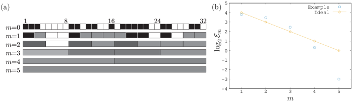
Figure 1: A demonstration of the 1D Haar wavelet transform. (a) Coarse-graining steps for each level-$m$ are shown. Black (white) squares at $m=0$ denote that the correspondent bits are zero (unity). An intensity of a gray rectangle denotes its coarse-grained value. (b) Plot of the logarithm of the entropy emission demonstrated in Fig. 1(a). Orange line and symbols denote an ideal dependence on $m$, $\log_{2}\mathcal{E}_{m}=\log_{2}L-m$.

Using the 1D Haar wavelet, we demonstrate the wavelet transformation of a binary random number sequence of length 32. The original random number sequence, $f(x)$, is shown in the top row of Fig. 1(a); black and white squares respectively denote 0 and 1. The entropy of 32-bit random number is 32 if we take the logarithm base 2. Intensities of gray rectangles in Fig. 1(a) denote values of the coarse-grained functions; by definition, the range of values is 0 to 1. In this demonstration, entropy emissions given in Eq. (17) are $\mathcal{E}_{1}=14$, $\mathcal{E}_{2}=11$, $\mathcal{E}_{3}=5.5$, $\mathcal{E}_{4}=1.25$, and $\mathcal{E}_{5}=0.125$. The accumulated entropy emission is 31.875, which is close to 32, the entropy of 32-bit random number sequence. Actually, the value of accumulated entropy emission comes closer to the bit length as the length is increased. From the demonstration we see that the quantity $\mathcal{E}_{m}$ shows the amount of entropy emission in a coarse-graining procedure between $(m-1)$th and $m$th wavelet transformation.

IV Results

Entropy emissions of the 2D $q$-state Potts models at critical points are calculated by Monte Carlo simulation. System size $L$ is $16384(=2^{14})$. A number of samples is $10^{4}$, and 10 independent Monte Carlo runs are executed to estimate statistical errors. In order to equilibrate spin configurations for $q\geq 2$ models, Swendsen-Wang algorithm Swendsen and Wang (1987); Komura and Okabe (2012); Komura (2015) is used, and $2\times 10^{4}$ Monte Carlo steps are discarded for thermalization. The temperature is fixed at the critical point of the 2D $q$-state Potts model,

$$T_{\mathrm{c}}=\frac{1}{\ln(1+\sqrt{q})}.$$ (18)

In the percolation formula, this gives the critical probability of connecting the same spins [see Eq. (2)],

$$p_{\mathrm{c}}=\frac{\sqrt{q}}{1+\sqrt{q}}.$$ (19)

We execute the wavelet transform for each bond configuration obtained during measurement runs. The wavelet transform applies to each $2\times 2$ block of vertical and horizontal bonds, and the both of vertical and horizontal contributions are taken into the entropy emission. Figure 2 shows normalized entropy emissions for the 2D Potts models. As we saw in the example of a random number sequence in Sec. III, the quantity does not change its value when site- or bond-variables are totally random. Curves in Fig. 2 are given by

$$\epsilon_{m}=\epsilon_{0}\left(1+\frac{c}{6}\mathcal{A}\ln s_{m}\right),$$ (20)

where $c$ is the central charge, $\mathcal{A}$ is the boundary length between clusters, and $s_{m}(=2^{m})$ is a side length of a wavelet basis. The second term in the parenthesis in the right-hand side is known as Calabrese-Cardy formula Holzhey et al. (1994); Calabrese and Cardy (2004). In the case of the 2D critical Potts model, $\mathcal{A}$ is proportional to $s_{m}^{D_{\mathrm{EP}}-1}$, where $D_{\mathrm{EP}}$ is the dimension of the external perimeter. Exact values of $c$’s and $D_{\mathrm{EP}}$’s are listed in Table 1 Duplantier (2000). To draw curves in Fig. 2, we assumed the proportional constant as unity; that is,

$$\epsilon_{m}=\epsilon_{0}\left(1+\frac{c}{6}2^{(D_{\mathrm{EP}}-1)m}\ln 2^{m}\right).$$ (21)

Probably the value of the true proportional constant is close to unity, since curves run on numerical data at $m=2$.

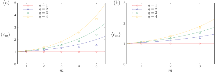
Figure 2: (a) $m$ dependence of normalized entropy emissions of the 2D $q$-state Potts models. Curves denote Calabrese-Cardy formula, Eq. (21). (b) Magnified view of Fig. 2(a). Error bars are smaller than the size of the symbols.

Table 1: Central charges $c$ and the dimensions of the external perimeter $D_{\mathrm{EP}}$ for the critical $q$-state Potts model Duplantier (2000).

$q$	1	2	3	4
$c$	0	1/2	4/5	1
$D_{\mathrm{EP}}$	4/3	11/8	17/12	3/2

V Summary and Discussion

The entropy emission seems to measure the entanglement entropy in the 2D $q$-state Potts models, and it is curious how the entropy emission can measure the entanglement entropy from a snapshot. Wavelet coefficients detect segments of boundaries between FK clusters. Level $m$ dependence of the coefficients has a correspondence with a characteristic length of boundary: Sizes of FK clusters are small at a high temperature, and the entropy emission decreases as $m$ increases. At a low temperature, to the contrary, sizes of FK clusters are large, and the entropy emission increases as $m$ increases. At an intermediate temperature, near a criticality, the entropy emission is almost flat. An extreme case is the percolation problem at the critical point, where the entropy emission is invariant under the wavelet transformation due to the fractality of clusters’ shape. Entropy emissions of Potts models for $q=2,3,4$ at their criticalities mildly increase as $m$ is increased. Difference between the percolation problem and the spin models is correlations between bonds. The density of bonds at their criticality is universal, $b(g)/N_{b}=1/2$. This comes from the self-dual of the square lattice. Bond distributions of the spin models are more denser than that of the percolation problem since bond occupation is restricted between the same spins. Dense FK clusters are robust against the wavelet transform, and the robustness causes the mild increase of the entropy emission. Fractality of the FK clusters brings about non-trivial growth of boundary length, $\mathcal{A}\propto s^{D_{\mathrm{EP}}-1}$, and Eq. (21) is deduced. In the percolation formula, only a freedom of spin assignment on each of FK clusters remains; that is, wavelet coefficients, which are non-zero at a cluster boundary, capture a universality class of a system from a snapshot of a bond configuration at each level $m$. To examine the conjecture formula, Eq. (21), elaborate studies on wavelet transformation of FK clusters are required.

The fact that spin configuration is not essential but FK cluster configuration given by the percolation formula is important suggests a guideline studying critical phenomena using image processing. It has been known that the percolation formula is quite helpful for a study of critical phenomena Tomita and Okabe (2001); Tomita et al. (1999); Swendsen and Wang (1987), and the analysis with wavelets confirms again its importance. The insight promises that applications to world line configurations in quantum spin Monte Carlo simulations Evertz et al. (1993); Kawashima and Harada (2004); Tomita and Okabe (2002) will work well. I leave the application for a future study. It is obvious that a wavelet transform of spin configuration will fail to investigate critical phenomena of spin systems. Since wavelet transform conserves magnetization, its coarse-graining procedure deviates from the legitimate RG. In this study, the wavelet transform is carried out for bond configuration, and the densities of bonds are being kept correctly at 1/2 during the wavelet transform. It is probable that an inference of bond distribution is indispensable when one investigates critical phenomena of spin systems by image processing of spin configuration only.

Wavelet analysis proposed in this study is imperfect. Except for the percolation problem, deviations of normalized entropy emissions from Eq. (21) systematically grows larger with each wavelet transform. The flaw would come from interfusion of bonds that belongs to different FK clusters. More sophisticated way to coarse-grain bonds will restore the flaw, and the modification will bring about clearer understanding on relations between spin systems at criticality and image processing.

*

Appendix A Wavelet transform with the 2D Haar wavelet

In this paper, we used the 2D Haar wavelet transform to obtain coarse-grained bond configuration. Here, in stead of a function of bonds, we consider a wavelet transform of a function defined on a square lattice points of size $2^{n}\times 2^{n}$ for a brief description. A level-$m$ coarse-grained bond configuration at a lattice point $(x,y)$, $f_{m}(x,y)$, is represented by a sum of level-$m$ scaling functions $\phi_{m;i,j}(x,y)$,

$$f_{m}(x,y)=\sum_{i,j}c_{m;i,j}\phi_{m;i,j}(x,y),$$ (22)

where $c_{m;i,j}$ is a scaling coefficient. Using level-$0$ scaling functions the original function $f(x,y)$ is represented by

$$f(x,y)=\sum_{i,j}c_{0;i,j}\phi_{0;i,j}(x,y).$$ (23)

The function $\phi_{0;i,j}(x,y)$ is defined by

$$\phi_{0;i,j}(x,y)=\left\{\begin{array}[]{ll}1&\mbox{if $(x,y)=(i,j)$},\\ 0&\mbox{otherwise}.\end{array}\right.$$ (24)

Level-$m$ scaling functions can be expressed by using level-$(m-1)$ scaling functions as

$$\phi_{m;i,j}(x,y) =\Braket{\left(\begin{array}[]{ll}1&1\\ 1&1\end{array}\right)}{\left(\begin{array}[]{ll}\phi_{m-1;2i,2j}(x,y)&\phi_{m-1;2i+1,2j}(x,y)\\ \phi_{m-1;2i,2j+1}(x,y)&\phi_{m-1;2i,2j+1}(x,y)\end{array}\right)}_{\mathrm{F}}$$ (29)

$$=\phi_{m-1;2i,2j}(x,y)+\phi_{m-1;2i+1,2j}(x,y)+\phi_{m-1;2i,2j+1}(x,y)+\phi_{m-1;2i,2j+1}(x,y)$$ (30)

where $\braket{\mathsf{A}}{\mathsf{B}}_{\mathrm{F}}$ denotes the Frobenius inner product of matrices $\mathsf{A}$ and $\mathsf{B}$. The scaling functions satisfy orthogonal property,

$$\braket{\phi_{m;i,j}(x,y)}{\phi_{m;i^{\prime},j^{\prime}}(x,y)} =\sum_{x,y}\phi_{m;i,j}(x,y),\phi_{m;i^{\prime},j^{\prime}}(x,y)$$ (31)

$$=4^{m}\delta_{i,i^{\prime}}\delta_{j,j^{\prime}},$$ (32)

where the summation runs all the lattice points, $x,y\in[0,2^{n}-1]$, and $\delta_{i,j}$ is the Kronecker delta. By virtue of the orthogonality, a scaling coefficient $c_{m;i,j}$ can be obtained by the following inner product,

$$c_{m;i,j}=\braket{f(x,y)}{\phi_{m;i,j}(x,y)}$$ (33)

Using the recursion relation of $\phi_{m;i,j}(x,y)$, Eq. (29), the above equation can be rewritten as

$$c_{m;i,j}=\frac{1}{4}(c_{m-1;2i,2j}+c_{m-1;2i+1,2j}+c_{m-1;2i,2j+1}+c_{m-1;2i+1,2j+1}).$$ (34)

Namely level-$m$ scaling coefficients are given by the average of coefficients of level-$(m-1)$. The 2D Haar wavelet functions are given by

$$\psi^{v}_{m;i,j}(x,y) =\frac{1}{4^{m}}\Braket{\left(\begin{array}[]{rr}1&1\\ -1&-1\end{array}\right)}{\left(\begin{array}[]{ll}\phi_{m-1;2i,2j}(x,y)&\phi_{m-1;2i+1,2j}(x,y)\\ \phi_{m-1;2i,2j+1}(x,y)&\phi_{m-1;2i,2j+1}(x,y)\end{array}\right)}_{\mathrm{F}},$$ (39)

$$\psi^{h}_{m;i,j}(x,y) =\frac{1}{4^{m}}\Braket{\left(\begin{array}[]{rr}1&-1\\ 1&-1\end{array}\right)}{\left(\begin{array}[]{ll}\phi_{m-1;2i,2j}(x,y)&\phi_{m-1;2i+1,2j}(x,y)\\ \phi_{m-1;2i,2j+1}(x,y)&\phi_{m-1;2i,2j+1}(x,y)\end{array}\right)}_{\mathrm{F}},$$ (44)

$$\psi^{d}_{m;i,j}(x,y) =\frac{1}{4^{m}}\Braket{\left(\begin{array}[]{rr}1&-1\\ -1&1\end{array}\right)}{\left(\begin{array}[]{ll}\phi_{m-1;2i,2j}(x,y)&\phi_{m-1;2i+1,2j}(x,y)\\ \phi_{m-1;2i,2j+1}(x,y)&\phi_{m-1;2i,2j+1}(x,y)\end{array}\right)}_{\mathrm{F}}.$$ (49)

These three wavelet functions are also orthogonal:

$$\braket{\psi^{\alpha}_{m;i,j}(x,y)}{\psi^{\beta}_{m;i^{\prime},j^{\prime}}(x,y)}=\frac{1}{4^{m}}\delta_{\alpha,\beta}\delta_{i,i^{\prime}}\delta_{j,j^{\prime}},\quad(\alpha,\beta\in\{v,h,d\}).$$ (50)

Wavelet coefficients $d^{\alpha}_{m;i,j}$ can be obtained by

$$d^{v}_{m;i,j} =\braket{f(x,y)}{\psi^{v}_{m;i,j}(x,y)},$$ (51)

$$d^{h}_{m;i,j} =\braket{f(x,y)}{\psi^{h}_{m;i,j}(x,y)},$$ (52)

$$d^{d}_{m;i,j} =\braket{f(x,y)}{\psi^{d}_{m;i,j}(x,y)}.$$ (53)

Again, using recursive relation we obtain

$$d^{v}_{m;i,j} =\frac{1}{4}(c_{m-1;2i,2j}+c_{m-1;2i+1,2j}-c_{m-1;2i,2j+1}-c_{m-1;2i+1,2j+1}),$$ (54)

$$d^{h}_{m;i,j} =\frac{1}{4}(c_{m-1;2i,2j}-c_{m-1;2i+1,2j}+c_{m-1;2i,2j+1}-c_{m-1;2i+1,2j+1}),$$ (55)

$$d^{d}_{m;i,j} =\frac{1}{4}(c_{m-1;2i,2j}-c_{m-1;2i+1,2j}-c_{m-1;2i,2j+1}+c_{m-1;2i+1,2j+1}).$$ (56)

From these equations, it can be read that level-$m$ wavelet coefficients preserve differences between neighboring $f_{m-1}(x,y)$’s. Indeed, level-$(m-1)$ scaling functions can be restored by level-$m$ scaling and wavelet functions:

$$\phi_{m-1;2i,2j}(x,y) =\frac{1}{4}\{\phi_{m;i,j}(x,y)+4^{m}[\psi^{v}_{m;i,j}(x,y)+\psi^{h}_{m;i,j}(x,y)+\psi^{d}_{m;i,j}(x,y)]\},$$ (57)

$$\phi_{m-1;2i+1,2j}(x,y) =\frac{1}{4}\{\phi_{m;i,j}(x,y)+4^{m}[\psi^{v}_{m;i,j}(x,y)-\psi^{h}_{m;i,j}(x,y)-\psi^{d}_{m;i,j}(x,y)]\},$$ (58)

$$\phi_{m-1;2i,2j+1}(x,y) =\frac{1}{4}\{\phi_{m;i,j}(x,y)+4^{m}[-\psi^{v}_{m;i,j}(x,y)+\psi^{h}_{m;i,j}(x,y)-\psi^{d}_{m;i,j}(x,y)]\},$$ (59)

$$\phi_{m-1;2i+1,2j+1}(x,y) =\frac{1}{4}\{\phi_{m;i,j}(x,y)+4^{m}[-\psi^{v}_{m;i,j}(x,y)-\psi^{h}_{m;i,j}(x,y)+\psi^{d}_{m;i,j}(x,y)]\}.$$ (60)

In a similar way, we obtain the following relations:

$$c_{m-1;2i,2j} =c_{m;i,j}+d^{v}_{m;i,j}+d^{h}_{m;i,j}+d^{d}_{m;i,j},$$ (61)

$$c_{m-1;2i+1,2j} =c_{m;i,j}+d^{v}_{m;i,j}-d^{h}_{m;i,j}-d^{d}_{m;i,j},$$ (62)

$$c_{m-1;2i,2j+1} =c_{m;i,j}-d^{v}_{m;i,j}+d^{h}_{m;i,j}-d^{d}_{m;i,j},$$ (63)

$$c_{m-1;2i+1,2j+1} =c_{m;i,j}-d^{v}_{m;i,j}-d^{h}_{m;i,j}+d^{d}_{m;i,j}.$$ (64)

Namely the lost information caused by a wavelet transform from level-$(m-1)$ to level-$m$ is properly preserved in level-$m$ wavelet coefficients. Therefore, I define a quantity which measures an amount of emitted information entropy at a level-$m$ wavelet transform as

$$\mathcal{E}_{m}=4^{m+1}\sum_{i,j}[(d^{v}_{m;i,j})^{2}+(d^{h}_{m;i,j})^{2}+(d^{d}_{m;i,j})^{2}].$$ (65)

The normalized entropy emission is given by

$$\epsilon_{m}=\frac{4^{m+1}}{3N_{m}}\sum_{i,j}[(d^{v}_{m;i,j})^{2}+(d^{h}_{m;i,j})^{2}+(d^{d}_{m;i,j})^{2}],$$ (66)

where $N_{m}(=2^{n-m}\times 2^{n-m})$ is the number of coarse-grained lattice sites. The number 3 in the denominator makes the normalized entropy emission unity in the critical percolation problem. In this paper, we applied the 2D Haar wavelet transform to vertical and horizontal bonds, and contributions from the both kinds of bonds are averaged. The original function $f(x,y)$ is set as unity (zero) if a bond is occupied (empty) at $(x,y)$. Therefore the coarse-graining procedure for bonds is essentially the same as in the demonstration in Sec. III.

References

- White (1992) S. R. White, Phys. Rev. Lett. 69, 2863 (1992).
- White (1993) S. R. White, Phys. Rev. B 48, 10345 (1993).
- Nishino and Okunishi (1996) T. Nishino and K. Okunishi, J. Phys. Soc. Jpn. 65, 891 (1996).
- Nishino and Okunishi (1997) T. Nishino and K. Okunishi, J. Phys. Soc. Jpn. 66, 3040 (1997).
- Levin and Nave (2007) M. Levin and C. P. Nave, Phys. Rev. Lett. 99, 120601 (2007).
- Evenbly and Vidal (2009) G. Evenbly and G. Vidal, Phys. Rev. B 79, 144108 (2009).
- Evenbly and Vidal (2015) G. Evenbly and G. Vidal, Phys. Rev. Lett. 115, 180405 (2015).
- Ma (1976) S.-k. Ma, Phys. Rev. Lett. 37, 461 (1976).
- Swendsen (1979) R. H. Swendsen, Phys. Rev. Lett. 42, 859 (1979).
- Sugiura and Shimizu (2013) S. Sugiura and A. Shimizu, Phys. Rev. Lett. 111, 010401 (2013).
- Tasaki (2016) H. Tasaki, Journal of Statistical Physics 163, 937 (2016).
- Ueda et al. (2005) K. Ueda, R. Otani, Y. Nishino, A. Gendiar, and T. Nishino, J. Phys. Soc. Jpn. Suppl. 74, 111 (2005).
- Matsueda (2012) H. Matsueda, Phys. Rev. E 85, 031101 (2012).
- Imura et al. (2014) Y. Imura, T. Okubo, S. Morita, and K. Okunishi, J. Phys. Soc. Jpn. 83, 114002 (2014).
- Lee et al. (2015) C. H. Lee, Y. Yamada, T. Kumamoto, and H. Matsueda, J. Phys. Soc. Jpn. 84, 013001 (2015).
- Matsueda and Ozaki (2015) H. Matsueda and D. Ozaki, Phys. Rev. E 92, 042167 (2015).
- Lee et al. (2016) C. H. Lee, D. Ozaki, and H. Matsueda, Phys. Rev. E 94, 062144 (2016).
- Daubechies (1992) I. Daubechies, Ten Lectures on Wavelets (Society for Industrial and Applied Mathematics, 1992).
- Kasteleyn and Fortuin (1969) P. Kasteleyn and C. Fortuin, J. Phys. Soc. Jpn. Suppl. 26, 11 (1969).
- Fortuin and Kasteleyn (1972) C. Fortuin and P. Kasteleyn, Physica 57, 536 (1972).
- Holzhey et al. (1994) C. Holzhey, F. Larsen, and F. Wilczek, Nuclear Physics B 424, 443 (1994).
- Calabrese and Cardy (2004) P. Calabrese and J. Cardy, J. Stat. Mech. 2004, P06002 (2004).
- Potts (1952) R. B. Potts, Mathematical Proceedings of the Cambridge Philosophical Society 48, 106–109 (1952).
- Kihara et al. (1954) T. Kihara, Y. Midzuno, and T. Shizume, J. Phys. Soc. Jpn. 9, 681 (1954).
- Wu (1982) F. Y. Wu, Rev. Mod. Phys. 54, 235 (1982).
- Coniglio and Klein (1980) A. Coniglio and W. Klein, Journal of Physics A: Mathematical and General 13, 2775 (1980).
- Hu (1984) C.-K. Hu, Phys. Rev. B 29, 5103 (1984).
- Swendsen and Wang (1987) R. H. Swendsen and J.-S. Wang, Phys. Rev. Lett. 58, 86 (1987).
- Komura and Okabe (2012) Y. Komura and Y. Okabe, Computer Physics Communications 183, 1155 (2012).
- Komura (2015) Y. Komura, Computer Physics Communications 194, 54 (2015).
- Duplantier (2000) B. Duplantier, Phys. Rev. Lett. 84, 1363 (2000).
- Tomita and Okabe (2001) Y. Tomita and Y. Okabe, Phys. Rev. Lett. 86, 572 (2001).
- Tomita et al. (1999) Y. Tomita, Y. Okabe, and C.-K. Hu, Phys. Rev. E 60, 2716 (1999).
- Evertz et al. (1993) H. G. Evertz, G. Lana, and M. Marcu, Phys. Rev. Lett. 70, 875 (1993).
- Kawashima and Harada (2004) N. Kawashima and K. Harada, J. Phys. Soc. Jpn. 73, 1379 (2004).
- Tomita and Okabe (2002) Y. Tomita and Y. Okabe, Phys. Rev. B 66, 180401 (2002).