Generalizing the Kawaguchi-Kyan bound to stochastic parallel machine scheduling

Abstract

Minimizing the sum of weighted completion times on $m$ identical parallel machines is one of the most important and classical scheduling problems. For the stochastic variant where processing times of jobs are random variables, Möhring, Schulz, and Uetz (1999) presented the first and still best known approximation result achieving, for arbitrarily many machines, performance ratio $1+\frac{1}{2}(1+\Delta)$, where $\Delta$ is an upper bound on the squared coefficient of variation of the processing times. We prove performance ratio $1+\frac{1}{2}(\sqrt{2}-1)(1+\Delta)$ for the same underlying algorithm – the Weighted Shortest Expected Processing Time (WSEPT) rule. For the special case of deterministic scheduling (i.e., $\Delta=0$), our bound matches the tight performance ratio $\frac{1}{2}(1+\sqrt{2})$ of this algorithm (WSPT rule), derived by Kawaguchi and Kyan in a 1986 landmark paper. We present several further improvements for WSEPT’s performance ratio, one of them relying on a carefully refined analysis of WSPT yielding, for every fixed number of machines $m$, WSPT’s exact performance ratio of order $\frac{1}{2}(1+\sqrt{2})-O(1/m^{2})$.

1 Introduction

In an archetypal machine scheduling problem, $n$ independent jobs have to be scheduled on $m$ identical parallel machines or processors. Each job $j$ is specified by its processing time $p_{j}>0$ and by its weight $w_{j}>0$. In a feasible schedule, every job $j$ is processed for $p_{j}$ time units on one of the $m$ machines in an uninterrupted fashion, and every machine can process at most one job at a time. The completion time of job $j$ in some schedule $\mathrm{S}$ is denoted by $C_{j}^{\mathrm{S}}$. The goal is to compute a schedule $\mathrm{S}$ that minimizes the total weighted completion time $\sum_{j=1}^{n}w_{j}C_{j}^{\mathrm{S}}$. In the standard classification scheme of Graham, Lawler, Lenstra, and Rinnooy Kan [8], this NP-hard scheduling problem is denoted by $P||\sum w_{j}C_{j}$.

Weighted Shortest Processing Time Rule

By a well-known result of Smith [24], sequencing the jobs in order of non-increasing ratios $w_{j}/p_{j}$ gives an optimal single-machine schedule. List scheduling in this order is known as the Weighted Shortest Processing Time (WSPT) rule and can also be applied to identical parallel machines, where it is a $\frac{1}{2}(1+\sqrt{2})$-approximation algorithm; see Kawaguchi and Kyan [14]. A particularly remarkable aspect of Kawaguchi and Kyan’s work is that, in contrast to the vast majority of approximation results, their analysis does not rely on some kind of lower bound. Instead, they succeed in explicitly identifying a class of worst-case instances. In particular, the performance ratio $\frac{1}{2}(1+\sqrt{2})$ is tight: For every $\varepsilon>0$ there is a problem instance for which WSPT has approximation ratio at least $\frac{1}{2}(1+\sqrt{2})-\varepsilon$. The instances achieving these approximation ratios, however, have large numbers of machines when $\varepsilon$ becomes small. Schwiegelshohn [20] gives a considerably simpler version of Kawaguchi and Kyan’s analysis.

Stochastic Scheduling

Many real-world machine scheduling problems exhibit a certain degree of uncertainty about the jobs’ processing times. This characteristic is captured by the theory of stochastic machine scheduling, where the processing time of job $j$ is no longer a given number $p_{j}$ but a random variable $\bm{p}_{j}$. As all previous work in the area, we always assume that these random variables are stochastically independent. At the beginning, only the distributions of these random variables are known. The actual processing time of a job becomes only known upon its completion. As a consequence, the solution to a stochastic scheduling problem is no longer a simple schedule, but a so-called non-anticipative scheduling policy. Precise definitions on stochastic scheduling policies are given by Möhring, Radermacher, and Weiss [16]. Intuitively, whenever a machine is idle at time $t$, a non-anticipative scheduling policy may decide to start a job of its choice based on the observed past up to time $t$ as well as the a priori knowledge of the jobs processing time distributions and weights. It is, however, not allowed to anticipate information about the future, i.e., the actual realizations of the processing times of jobs that have not yet finished by time $t$.

It follows from simple examples that, in general, a non-anticipative scheduling policy cannot yield an optimal schedule for each possible realization of the processing times. We are therefore looking for a policy which minimizes the objective in expectation. For the stochastic scheduling problem considered in this paper, the goal is to find a non-anticipative scheduling policy that minimizes the expected total weighted completion time. This problem is denoted by $P|\bm{p}_{j}\sim\mathrm{stoch}|\mathrm{E}[\sum w_{j}\bm{C}_{j}]$.

Weighted Shortest Expected Processing Time Rule

The stochastic analogue of the WSPT rule is greedily scheduling the jobs in order of non-increasing ratios $w_{j}/\mathrm{E}[\bm{p}_{j}]$. Whenever a machine is idle, the Weighted Shortest Expected Processing Time (WSEPT) rule immediately starts the next job in this order. For a single machine this is again optimal; see Rothkopf [18]. For identical parallel machines, Cheung, Fischer, Matuschke, and Megow [3] and Im, Moseley, and Pruhs [11] independently show that WSEPT does not even achieve constant performance ratio. More precisely, for every $R>0$ there is a problem instance for which WSEPT’s expected total weighted completion time is at least $R$ times the expected objective function value of an optimal non-anticipative scheduling policy. Even in the special case of exponentially distributed processing times, Jagtenberg, Schwiegelshohn, and Uetz [12] show a lower bound of $1.243$ on WSEPT’s performance. On the positive side, WSEPT is an optimal policy for the special case of unit weight jobs with stochastically ordered processing times, $P|\bm{p}_{j}\sim\mathrm{stoch}(\preceq_{\mathrm{st}})|E[\sum\bm{C}_{j}]$; see Weber, Varaiya, and Walrand [25]. Moreover, Weiss [26, 27] proves asymptotic optimality of WSEPT. Möhring, Schulz, and Uetz [17] show that the WSEPT rule achieves performance ratio $1+\frac{1}{2}(1+\Delta)(1-\frac{1}{m})$, where $\Delta$ is an upper bound on the squared coefficient of variation of the processing times.

Further Approximation Results from the Literature

While there is a PTAS for the deterministic problem $P||\sum w_{j}C_{j}$ [23], no constant-factor approximation algorithm is known for the stochastic problem $P|\bm{p}_{j}\sim\mathrm{stoch}|\mathrm{E}[\sum w_{j}\bm{C}_{j}]$. WSEPT’s performance ratio $1+\frac{1}{2}(1+\Delta)$ (for arbitrarily many machines) proven by Möhring et al. [17] is the best hitherto known performance ratio. The only known approximation ratio not depending on the jobs’ squared coefficient of variation $\Delta$ is due to Im et al. [11] who, for the special case of unit job weights $P|\bm{p}_{j}\sim\mathrm{stoch}|\mathrm{E}[\sum\bm{C}_{j}]$, present an $O(\log^{2}n+m\log n)$-approximation algorithm.

The performance ratio $1+\frac{1}{2}(1+\Delta)$ has been carried over to different generalizations of $P|\bm{p}_{j}\sim\mathrm{stoch}|\mathrm{E}[\sum w_{j}\bm{C}_{j}]$. Megow, Uetz, and Vredeveld [15] show that it also applies if jobs arrive online in a list and must immediately and irrevocably be assigned to machines, on which they can be sequenced optimally. An approximation algorithm with this performance ratio for the problem on unrelated parallel machines is designed by Skutella, Sviridenko, and Uetz [22]. If these two features are combined, i.e., in the online list-model with unrelated machines, Gupta, Moseley, Uetz, and Xie [9] develop a $(8+4\Delta)$-approximation algorithm.

The performance ratios are usually larger if jobs are released over time: In the offline setting, the best known approximation algorithm has performance ratio $2+\Delta$; see Schulz [19]. This performance ratio is also achieved for unrelated machines [22] and by a randomized online algorithm [19]. There exist furthermore a deterministic $(\max\{2.618,2.309+1.309\Delta\})$-approximation for the online setting [19] and a deterministic $(144+72\Delta)$-approximation for the online setting on unrelated parallel machines [9].

Our Contribution and Outline

We present the first progress on theapproximability of the basic stochastic scheduling problem on identicalparallel machines with expected total weighted completion time objective$P|\bm{p}_{j}\sim\mathrm{stoch}|\mathrm{E}[\sum w_{j}\bm{C}_{j}]$ since the seminal work of Möhring et al. [17]; see Figure 1.

Figure 1: Bounds on WSEPT’s performance ratio

We prove that WSEPT achieves performance ratio

$$1+\tfrac{1}{2}\min\left\{\frac{\sqrt{(2m-k_{m})k_{m}}-k_{m}}{m},\frac{1}{1+\min\{2,\sqrt{2+2\Delta}\}}\right\}(1+\Delta),$$ (1)

where $k_{m}\coloneqq\bigl{\lfloor}\bigl{(}1-\frac{1}{2}\sqrt{2}\bigr{)}m\bigr{\rceil}$ is the nearest integer to $\bigl{(}1-\frac{1}{2}\sqrt{2}\bigr{)}m$. Notice that, for every number of machines $m$, the performance ratio given by the first term of the minimum in (1) is bounded from above by $1+\tfrac{1}{2}(\sqrt{2}-1)(1+\Delta)$, and for $m\to\infty$ it converges to this bound. As $(1+\min\{2,\sqrt{2+2\Delta}\})^{-1}\leq\sqrt{2}-1$ for all $\Delta>0$, when considering an arbitrary number of machines, the second term in the minimum dominates the first term. In the following, we list several points that emphasize the significance of the new performance ratio (1).

• For the special case of deterministic scheduling (i.e., $\Delta=0$), the machine-independent performance ratio in (1) matches the Kawaguchi-Kyanbound $\frac{1}{2}(1+\sqrt{2})$, which is known to be tight [14]. In particular, we dissolve the somewhat annoying discontinuity of the best previously known bounds [14, 17] at $\Delta=0$; see Figure 1.

• Again for deterministic jobs, our machine-dependent bound$1+\frac{1}{2}(\sqrt{(2m-k_{m})k_{m}}-k_{m})/m$ is tight and slightly improves the 30 years old Kawaguchi-Kyan bound for every fixed number of machines $m$; see Figure 2.

  Figure 2: Graph of the function $m\mapsto 1+\frac{1}{2}(\sqrt{(2m-k_{m})k_{m}}-k_{m})/m$, which for $m\in\mathbb{N}$ gives the worst-case approximation ratio of WSPT for $P||\sum w_{j}C_{j}$ with $m$ machines (dots), compared to the machine-independent Kawaguchi-Kyan bound

• For exponentially distributed processing times ($\Delta=1$), our results imply that WSEPT achieves performance ratio $4/3$. This solves an open problem by Jagtenberg et al. [12], who give a lower bound of $1.243$ on WSEPT’s performance and ask for an improvement of the previously best known upper bound of $2-1/m$ due to Möhring et al. [17].

• WSEPT’s performance bound due to Möhring et al. [17] also holds for the MinIncrease policy, introduced by Megow et al. [15], which is a fixed-assignment policy, i.e., before the execution of the jobs starts, it determines for each job on which machine it is going to be processed. Our stronger bound, together with a lower bound in [22], shows that WSEPT actually beats every fixed-assignment policy.

The improved performance ratio in (1) is derived as follows. In Section 2 we present one of the key results of this paper (see Theorem 1 below): If WSPT has performance ratio $1+\beta$ for some $\beta$, then WSEPT achieves performance ratio $1+\beta(1+\Delta)$ for the stochastic scheduling problem. For the Kawaguchi-Kyan bound $1+\beta=\frac{1}{2}(1+\sqrt{2})$, this yields performance ratio $1+\frac{1}{2}(\sqrt{2}-1)(1+\Delta)$. It is also interesting to notice that the performance ratio of Möhring et al. [17] follows from this theorem by plugging in $1+\beta=3/2-1/(2m)$, which is WSPT’s performance ratio obtained from the bound of Eastman, Even, and Isaacs [4]. We generalize Theorem 1 to performance ratios w.r.t. the weighted sum of$\alpha$-points as objective function, where the $\alpha$-point of a job $j$ is the point in time when it has been processed for exactly $\alpha p_{j}$ time units.

The theorems derived in Section 2 provide tools to carry over bounds for the WSPT rule to the WSEPT rule. The concrete performance ratio for the WSEPT rule obtained this way thus depends on good bounds for the WSPT rule. In Section 3 we derive performance ratios for WSPT w.r.t. the weighted sum of $\alpha$-points objective. For $\alpha=\tfrac{1}{2}$ this performance ratio follows easily from a result by Avidor, Azar, and Sgall [1] for the 2-norm of the machine load vector. As a consequence we obtain performance ratio $1+\tfrac{1}{6}\max\{2,1+\Delta\}$ for WSEPT. By optimizing the choice of $\alpha$, we finally obtain the performance ratio $1+\frac{1}{2}(1+\min\{2,\sqrt{2+2\Delta}\})^{-1}(1+\Delta)$. The various bounds on WSEPT’s performance derived in Sections 2 and 3 are illustrated in Figure 1. Finally, in Section 4 the analysis of Schwiegelshohn [20] for the WSPT rule is refined for every fixed number of machines $m$, entailing the machine-dependent bound for the WSEPT rule in (1).

2 Performance ratio of the WSEPT rule

Let $\Delta\geq\mathrm{Var}[\bm{p}_{j}]/\mathrm{E}[\bm{p}_{j}]^{2}$ for all $j\in\{1,\dotsc,n\}$. In Theorems 1 and 2 we demonstrate how performance ratios for the WSPT rule for deterministic scheduling can be carried over to stochastic scheduling. Theorem 1 starts out from a performance ratio for WSPT with respect to the usual objective function: the weighted sum of completion times. In Theorem 2 this is generalized insofar as a performance ratio of WSPT with respect to the weighted sum of $\alpha$-points is taken as a basis.

Theorem 1.

If the WSPT rule on $m$ machines has performance ratio $1+\beta_{m}$ for the problem $P||\sum w_{j}C_{j}$, then the WSEPT rule achieves performance ratio $1+\beta_{m}(1+\Delta)$ for $P|\bm{p}_{j}\sim\mathrm{stoch}|\mathrm{E}[\sum w_{j}\bm{C}_{j}]$.

The reason why the bound for WSPT does not directly carry over to WSEPT is that under a specific realization of the processing times the schedule obtained by the WSEPT policy may differ from the WSPT schedule for this realization. Still, under every realization the WSEPT schedule is a list schedule. Hence, usually a bound that is valid for every list schedule is used: The objective value of a list schedule on $m$ machines is at most $1/m$ times the objective value of the list schedule on a single machine plus $(m-1)/m$ times the weighted sum of processing times. This bound, holding because a list schedule assigns each job to the currently least loaded machine, is applied realizationwise to obtain a corresponding bound on the expected values in stochastic scheduling (cf. [17, Lemma 4.1]), which can be compared to an LP-based lower bound on the expected total completion time under an optimal policy.

In order to benefit from the precise bounds known for the WSPT rule nevertheless, we regard the following modified stochastic scheduling problem: For each job, instead of its weight $w_{j}$, we are given a weight factor $\rho_{j}$. The actual weight of a job is $\rho_{j}$ times its actual processing time, i.e., if a job takes longer, it also becomes more important. The goal is again to minimize the total weighted completion time. For the thus defined stochastic scheduling problem list scheduling in order of $\rho$-values has the nice property that it creates a WSPT schedule in every realization. So, for this scheduling problem any performance ratio of WSPT directly carries over to this list scheduling policy. In the following proof of Theorem 1 we first compare the expected total weighted completion time of a WSEPT schedule for the original problem to the expected objective value list scheduling in order of $\rho_{j}$ for the modified problem, then apply the performance ratio of the WSPT rule, and finally compare the expected total weighted completion time of the optimal schedule for the modified problem to the expected objective value of the optimal policy for the original problem. The transitions between the two problems lead to the additional factor of $1+\Delta$ in the performance ratio.

Proof.

Consider an instance of $P|\bm{p}_{j}\sim\mathrm{stoch}|\mathrm{E}[\sum w_{j}\bm{C}_{j}]$ consisting of $n$ jobs and $m$ machines, and let $\beta\coloneqq\beta_{m}$ and $\rho_{j}\coloneqq w_{j}/\mathrm{E}[\bm{p}_{j}]$ for $j\in\{1,\dotsc,n\}$. For every realization $(p_{1},\dotsc,p_{n})$ of the processing times we consider the instance $I(p_{1},\dotsc,p_{n})$ of $P||\sum w_{j}C_{j}$ which consists of $n$ jobs with processing times $p_{1},\dotsc,p_{n}$ and weights $\rho_{1}p_{1},\dotsc,\rho_{n}p_{n}$, so that the jobs in the instance $I(p_{1},\dotsc,p_{n})$ have Smith ratios $\rho_{1},\dotsc,\rho_{n}$ for all possible realizations. Therefore, for every realization $(p_{1},\dotsc,p_{n})$ the schedule obtained by the WSEPT policy is a WSPT schedule for $I(p_{1},\dotsc,p_{n})$. Let $C_{j}^{\mathrm{WSEPT}}(p_{1},\dotsc,p_{n})$ denote the completion time of job $j$ in the schedule obtained by the WSEPT policy under the realization $(p_{1},\dotsc,p_{n})$, let $C_{j}^{*}(I(p_{1},\dotsc,p_{n}))$ denote its completion time in an optimal schedule for $I(p_{1},\dotsc,p_{n})$, and let $C_{j}^{\Pi^{*}}(p_{1},\dotsc,p_{n})$ denote $j$’s completion time in the schedule constructed by an optimal stochastic scheduling policy under the realization $(p_{1},\dotsc,p_{n})$. For every realization $(p_{1},\dotsc,p_{n})$ of the processing times, since the WSEPT schedule follows the WSPT rule for $I(p_{1},\dotsc,p_{n})$, its objective value is bounded by

$$\sum_{j=1}^{n}(\rho_{j}p_{j})C_{j}^{\mathrm{WSEPT}}(p_{1},\dotsc,p_{n})\leq(1+\beta)\cdot\sum_{j=1}^{n}(\rho_{j}p_{j})C_{j}^{*}(I(p_{1},\dotsc,p_{n})).$$

On the other hand, as the schedule obtained by an optimal stochastic scheduling policy is feasible for the instance $I(p_{1},\dotsc,p_{n})$, it holds that

$$\sum_{j=1}^{n}(\rho_{j}p_{j})C_{j}^{*}(I(p_{1},\dotsc,p_{n}))\leq\sum_{j=1}^{n}(\rho_{j}p_{j})C_{j}^{\Pi^{*}}(p_{1},\dotsc,p_{n}).$$

Putting these two inequalities together and taking expectations, we get the inequality

$$\mathrm{E}\left[\sum_{j=1}^{n}\rho_{j}\bm{p}_{j}\bm{C}_{j}^{\mathrm{WSEPT}}\right]\leq(1+\beta)\cdot\mathrm{E}\left[\sum_{j=1}^{n}\rho_{j}\bm{p}_{j}\bm{C}_{j}^{\Pi^{*}}\right],$$

where $\bm{C}_{j}^{\mathrm{WSEPT}}=C_{j}^{\mathrm{WSEPT}}(\bm{p}_{1},\dotsc,\bm{p}_{n})$ and $\bm{C}_{j}^{\Pi^{*}}=C_{j}^{\Pi^{*}}(\bm{p}_{1},\dotsc,\bm{p}_{n})$. Using the latter inequality, we can bound the expected total weighted completion time of the WSEPT rule:

$$\mathrm{E}\left[\sum_{j=1}^{n}w_{j}\bm{C}_{j}^{\mathrm{WSEPT}}\right]=\sum_{j=1}^{n}\rho_{j}\mathrm{E}[\bm{p}_{j}]\mathrm{E}[\bm{C}_{j}^{\mathrm{WSEPT}}]$$

$$\stackrel{{\scriptstyle(*)}}{{=}}\ \sum_{j=1}^{n}\rho_{j}\mathrm{E}[\bm{p}_{j}\bm{C}_{j}^{\mathrm{WSEPT}}]-\sum_{j=1}^{n}\rho_{j}\mathrm{Var}[\bm{p}_{j}]$$

$$=\ \mathrm{E}\left[\sum_{j=1}^{n}\rho_{j}\bm{p}_{j}\bm{C}_{j}^{\mathrm{WSEPT}}\right]-\sum_{j=1}^{n}\rho_{j}\mathrm{Var}[\bm{p}_{j}]$$

$$\leq\ (1+\beta)\cdot\mathrm{E}\left[\sum_{j=1}^{n}\rho_{j}\bm{p}_{j}\bm{C}_{j}^{\Pi^{*}}\right]-\sum_{j=1}^{n}\rho_{j}\mathrm{Var}[\bm{p}_{j}]$$

$$=\ (1+\beta)\cdot\sum_{j=1}^{n}\rho_{j}\mathrm{E}[\bm{p}_{j}\bm{C}_{j}^{\Pi^{*}}]-\sum_{j=1}^{n}\rho_{j}\mathrm{Var}[\bm{p}_{j}]$$

$$\stackrel{{\scriptstyle(*)}}{{=}}\ (1+\beta)\cdot\left(\sum_{j=1}^{n}\rho_{j}\mathrm{E}[\bm{p}_{j}]\mathrm{E}[\bm{C}_{j}^{\Pi^{*}}]+\sum_{j=1}^{n}\rho_{j}\mathrm{Var}[\bm{p}_{j}]\right)-\sum_{j=1}^{n}\rho_{j}\mathrm{Var}[\bm{p}_{j}]$$

$$=\ (1+\beta)\cdot\sum_{j=1}^{n}w_{j}\mathrm{E}[\bm{C}_{j}^{\Pi^{*}}]+\beta\sum_{j=1}^{n}\rho_{j}\mathrm{Var}[\bm{p}_{j}]$$

$$\leq\ (1+\beta)\cdot\sum_{j=1}^{n}w_{j}\mathrm{E}[\bm{C}_{j}^{\Pi^{*}}]+\Delta\beta\sum_{j=1}^{n}w_{j}\mathrm{E}[\bm{p}_{j}]$$

$$\leq\ (1+\beta(1+\Delta))\cdot\sum_{j=1}^{n}w_{j}\mathrm{E}[\bm{C}_{j}^{\Pi^{*}}]=(1+\beta(1+\Delta))\cdot\mathrm{E}\left[\sum_{j=1}^{n}w_{j}\bm{C}_{j}^{\Pi^{*}}\right].$$

The equalities marked with $(*)$ hold because for any stochastic scheduling policy $\Pi$ and all $j$

$$\mathrm{E}[\bm{p}_{j}\bm{C}_{j}^{\Pi}]=\mathrm{E}[\bm{p}_{j}(\bm{S}_{j}^{\Pi}+\bm{p}_{j})]=\mathrm{E}[\bm{p}_{j}\bm{S}_{j}^{\Pi}]+\mathrm{E}[\bm{p}_{j}^{2}]\\ =\mathrm{E}[\bm{p}_{j}]\mathrm{E}[\bm{S}_{j}^{\Pi}]+\mathrm{E}[\bm{p}_{j}]^{2}+\mathrm{Var}[\bm{p}_{j}]=\mathrm{E}[\bm{p}_{j}]\mathrm{E}[\bm{C}_{j}^{\Pi}]+\mathrm{Var}[\bm{p}_{j}],$$

where $\bm{S}_{j}^{\Pi}$ denotes the starting time of job $j$ under policy $\Pi$. The independence of $\bm{p}_{j}$ and $\bm{S}_{j}^{\Pi}$ follows from the non-anticipativity of policy $\Pi$, and the last inequality uses the fact that $\mathrm{E}[\bm{p}_{j}]\leq\mathrm{E}[\bm{C}_{j}^{\Pi^{*}}]$ for every job $j$. ∎

By plugging in the Kawaguchi-Kyan bound, we immediately get the following performance ratio (see Figure 1).

Corollary 1.

The WSEPT rule has performance ratio $1+\frac{1}{2}(\sqrt{2}-1)(1+\Delta)$ for the problem $P|\bm{p}_{j}\sim\mathrm{stoch}|\mathrm{E}[\sum w_{j}\bm{C}_{j}]$.

For $\alpha\in[0,1]$ the $\alpha$-point $C_{j}^{\mathrm{S}}(\alpha)$ of a job $j$ is the point in time at which it has been processed for $\alpha p_{j}$ time units. Introduced by Hall, Shmoys, and Wein [10] in order to convert a preemptive schedule into a non-preemptive one, the concept of $\alpha$-points is often used in the design of algorithms (see e.g. [5, 2, 6, 21]). In contrast, we use them to define an alternative objective function in order to improve the analysis of the WSEPT rule.

We consider as objective function the weighted sum of $\alpha$-points $\sum_{j=1}^{n}w_{j}C_{j}^{\mathrm{S}}(\alpha)$ for $\alpha\in[0,1]$, generalizing the weighted sum of completion times. For every $\alpha$ the weighted sum of $\alpha$-points differs only by the constant $(1-\alpha)\sum_{j=1}^{n}w_{j}p_{j}$ from the weighted sum of completion times. So as for optimal solutions the objective functions are equivalent. The same applies to the stochastic variant: Here the two objectives differ by the constant $(1-\alpha)\sum_{j=1}^{n}w_{j}\mathrm{E}[\bm{p}_{j}]$, whence they have the same optimal policies. We now generalize Theorem 1 to the (expected) weighted sum of $\alpha$-points.

Theorem 2.

If the WSPT rule has performance ratio $1+\beta$ for the problem $P||\sum w_{j}C_{j}(\alpha)$, then the WSEPT rule has performance ratio $1+\beta(1+\Delta)$ for the problem $P|\bm{p}_{j}\sim\mathrm{stoch}|\mathrm{E}[\sum w_{j}\bm{C}_{j}(\alpha)]$ and $1+\beta\cdot\max\{1,\alpha(1+\Delta)\}$ for the problem $P|\bm{p}_{j}\sim\mathrm{stoch}|\mathrm{E}[\sum w_{j}\bm{C}_{j}]$.

The proof uses the same idea as the proof of Theorem 1: The bound for $P||\sum w_{j}C_{j}(\alpha)$ is again applied realizationwise to the modified stochastic problem described above.

Proof.

We use the notation of the proof of Theorem 1 for $\alpha$-points $C_{j}(\alpha)$ instead of completion times $C_{j}$. Then we have by assumption that

$$\sum_{j=1}^{n}(\rho_{j}p_{j})C_{j}^{\mathrm{WSEPT}}(\alpha)(p_{1},\dotsc,p_{n}) \leq(1+\beta)\sum_{j=1}^{n}(\rho_{j}p_{j})C_{j}^{*}(\alpha)(I(p_{1},\dotsc,p_{n}))$$

$$\leq(1+\beta)\sum_{j=1}^{n}(\rho_{j}p_{j})C_{j}^{\Pi^{*}}(\alpha)(p_{1},\dotsc,p_{n}),$$

where the last inequality holds because the schedule obtained by the optimal stochastic scheduling policy is feasible for $I(p_{1},\dotsc,p_{n})$. This carries over to expected values:

$$\mathrm{E}\left[\sum_{j=1}^{n}\rho_{j}\bm{p}_{j}\bm{C}_{j}^{\mathrm{WSEPT}}(\alpha)\right]\leq(1+\beta)\cdot\mathrm{E}\left[\sum_{j=1}^{n}\rho_{j}\bm{p}_{j}\bm{C}_{j}^{\Pi^{*}}(\alpha)\right].$$ (2)

Furthermore, for any non-anticipative stochastic scheduling policy

$$\mathrm{E}[\bm{p}_{j}\bm{C}_{j}^{\Pi}(\alpha)] =\mathrm{E}[\bm{p}_{j}\bm{S}_{j}^{\Pi}]+\alpha\mathrm{E}[\bm{p}_{j}^{2}]=\mathrm{E}[\bm{p}_{j}]\mathrm{E}[\bm{S}_{j}^{\Pi}]+\alpha(\mathrm{E}[\bm{p}_{j}]^{2}+\mathrm{Var}[\bm{p}_{j}])$$

$$=\mathrm{E}[\bm{p}_{j}]\mathrm{E}[\bm{C}_{j}^{\Pi}(\alpha)]+\alpha\mathrm{Var}[\bm{p}_{j}]$$ (3)

$$=\mathrm{E}[\bm{p}_{j}]\mathrm{E}[\bm{C}_{j}^{\Pi}]+\alpha\mathrm{Var}[\bm{p}_{j}]-(1-\alpha)\mathrm{E}[\bm{p}_{j}]^{2}.$$ (4)

Therefore,

$$\mathrm{E}\left[\sum_{j=1}^{n}w_{j}\bm{C}_{j}^{\mathrm{WSEPT}}(\alpha)\right]=\sum_{j=1}^{n}\rho_{j}\mathrm{E}[\bm{p}_{j}]\mathrm{E}[\bm{C}_{j}^{\mathrm{WSEPT}}(\alpha)]$$

$$\stackrel{{\scriptstyle\eqref{eq:weighted expected alpha-point}}}{{=}}\ \sum_{j=1}^{n}\rho_{j}\mathrm{E}[\bm{p}_{j}\bm{C}_{j}^{\mathrm{WSEPT}}(\alpha)]-\alpha\sum_{j=1}^{n}\rho_{j}\mathrm{Var}[\bm{p}_{j}])$$

$$=\ \mathrm{E}\left[\sum_{j=1}^{n}\rho_{j}\bm{p}_{j}\bm{C}_{j}^{\mathrm{WSEPT}}(\alpha)\right]-\alpha\sum_{j=1}^{n}\rho_{j}\mathrm{Var}[\bm{p}_{j}]$$

$$\stackrel{{\scriptstyle\eqref{eq:inequality expected values random weights}}}{{\leq}}\ (1+\beta)\cdot\mathrm{E}\left[\sum_{j=1}^{n}\rho_{j}\bm{p}_{j}\bm{C}_{j}^{\Pi^{*}}(\alpha)\right]-\alpha\sum_{j=1}^{n}\rho_{j}\mathrm{Var}[\bm{p}_{j}]$$

$$=\ (1+\beta)\cdot\sum_{j=1}^{n}\rho_{j}\mathrm{E}[\bm{p}_{j}\bm{C}_{j}^{\Pi^{*}}(\alpha)]-\alpha\sum_{j=1}^{n}\rho_{j}\mathrm{Var}[\bm{p}_{j}]$$

$$\stackrel{{\scriptstyle\eqref{eq:weighted expected alpha-point}}}{{=}}\ (1+\beta)\cdot\left(\sum_{j=1}^{n}\rho_{j}\mathrm{E}[\bm{p}_{j}]\mathrm{E}[\bm{C}_{j}^{\Pi^{*}}(\alpha)]+\alpha\sum_{j=1}^{n}\rho_{j}\mathrm{Var}[\bm{p}_{j}]\right)-\alpha\sum_{j=1}^{n}\rho_{j}\mathrm{Var}[\bm{p}_{j}]$$

$$=\ (1+\beta)\cdot\sum_{j=1}^{n}w_{j}\mathrm{E}[\bm{C}_{j}^{\Pi^{*}}(\alpha)]+\alpha\beta\sum_{j=1}^{n}\rho_{j}\mathrm{Var}[\bm{p}_{j}]$$

$$\leq\ (1+\beta)\cdot\sum_{j=1}^{n}w_{j}\mathrm{E}[\bm{C}_{j}^{\Pi^{*}}(\alpha)]+\alpha\beta\Delta\sum_{j=1}^{n}w_{j}\underbrace{\mathrm{E}[\bm{p}_{j}]}_{\leq\frac{\mathrm{E}[\bm{C}_{j}^{\Pi^{*}}(\alpha)]}{\alpha}}$$

$$\leq\ (1+\beta(1+\Delta))\cdot\sum_{j=1}^{n}w_{j}\mathrm{E}[\bm{C}_{j}^{\Pi^{*}}(\alpha)]=(1+\beta(1+\Delta))\cdot\mathrm{E}\left[\sum_{j=1}^{n}w_{j}\bm{C}_{j}^{\Pi^{*}}(\alpha)\right],$$

and

$$\mathrm{E}\left[\sum_{j=1}^{n}w_{j}\bm{C}_{j}^{\mathrm{WSEPT}}\right]=\sum_{j=1}^{n}\rho_{j}\mathrm{E}[\bm{p}_{j}]\mathrm{E}[\bm{C}_{j}^{\mathrm{WSEPT}}]$$

$$\stackrel{{\scriptstyle\eqref{eq:weighted expected completion time}}}{{=}}\ \sum_{j=1}^{n}\rho_{j}\mathrm{E}[\bm{p}_{j}\bm{C}_{j}^{\mathrm{WSEPT}}(\alpha)]-\sum_{j=1}^{n}\rho_{j}(\alpha\mathrm{Var}[\bm{p}_{j}]-(1-\alpha)\mathrm{E}[\bm{p}_{j}]^{2})$$

$$=\ \mathrm{E}\left[\sum_{j=1}^{n}\rho_{j}\bm{p}_{j}\bm{C}_{j}^{\mathrm{WSEPT}}(\alpha)\right]-\sum_{j=1}^{n}\rho_{j}(\alpha\mathrm{Var}[\bm{p}_{j}]-(1-\alpha)\mathrm{E}[\bm{p}_{j}]^{2})$$

$$\stackrel{{\scriptstyle\eqref{eq:inequality expected values random weights}}}{{\leq}}\ (1+\beta)\cdot\mathrm{E}\left[\sum_{j=1}^{n}\rho_{j}\bm{p}_{j}\bm{C}_{j}^{\Pi^{*}}(\alpha)\right]-\sum_{j=1}^{n}\rho_{j}(\alpha\mathrm{Var}[\bm{p}_{j}]-(1-\alpha)\mathrm{E}[\bm{p}_{j}]^{2})$$

$$=\ (1+\beta)\cdot\sum_{j=1}^{n}\rho_{j}\mathrm{E}[\bm{p}_{j}\bm{C}_{j}^{\Pi^{*}}(\alpha)]-\sum_{j=1}^{n}\rho_{j}(\alpha\mathrm{Var}[\bm{p}_{j}]-(1-\alpha)\mathrm{E}[\bm{p}_{j}]^{2})$$

$$\stackrel{{\scriptstyle\eqref{eq:weighted expected completion time}}}{{=}}\ (1+\beta)\cdot\left(\sum_{j=1}^{n}\rho_{j}\mathrm{E}[\bm{p}_{j}]\mathrm{E}[\bm{C}_{j}^{\Pi^{*}}]+\sum_{j=1}^{n}\rho_{j}(\alpha\mathrm{Var}[\bm{p}_{j}]-(1-\alpha)\mathrm{E}[\bm{p}_{j}]^{2})\right)$$

$$\hskip 40.00006pt-\sum_{j=1}^{n}\rho_{j}(\alpha\mathrm{Var}[\bm{p}_{j}]-(1-\alpha)\mathrm{E}[\bm{p}_{j}]^{2})$$

$$=\ (1+\beta)\cdot\sum_{j=1}^{n}w_{j}\mathrm{E}[\bm{C}_{j}^{\Pi^{*}}]+\beta\sum_{j=1}^{n}\rho_{j}(\alpha\mathrm{Var}[\bm{p}_{j}]-(1-\alpha)\mathrm{E}[\bm{p}_{j}]^{2})$$

$$\leq\ (1+\beta)\cdot\sum_{j=1}^{n}w_{j}\mathrm{E}[\bm{C}_{j}^{\Pi^{*}}]+\beta\sum_{j=1}^{n}\rho_{j}(\alpha\Delta-(1-\alpha))\mathrm{E}[\bm{p}_{j}]^{2}$$

$$=\ (1+\beta)\cdot\sum_{j=1}^{n}w_{j}\mathrm{E}[\bm{C}_{j}^{\Pi^{*}}]+\beta(\alpha(1+\Delta)-1)\sum_{j=1}^{n}w_{j}\underbrace{\mathrm{E}[\bm{p}_{j}]}_{\in[0,\mathrm{E}[\bm{C}_{j}^{\Pi^{*}}]]}$$

$$\leq\ (1+\beta)\cdot\sum_{j=1}^{n}w_{j}\mathrm{E}[\bm{C}_{j}^{\Pi^{*}}]+\beta\cdot\max\{0,\alpha(1+\Delta)-1\}\sum_{j=1}^{n}w_{j}\mathrm{E}[\bm{C}_{j}^{\Pi^{*}}]$$

$$\leq\ (1+\beta\cdot\max\{1,\alpha(1+\Delta)\})\cdot\mathrm{E}\left[\sum_{j=1}^{n}w_{j}\bm{C}_{j}^{\Pi^{*}}\right].\qed$$

Theorem 1 follows from Theorem 2 by plugging in $\alpha=1$.

3 Performance ratios for WSPT with weighted sum of $\alpha$-points objective

In this section we derive performance ratios for $P||\sum w_{j}C_{j}(\alpha)$. The two classical performance ratios for $P||\sum w_{j}C_{j}$ of Eastman, Even, and Isaacs [4] and of Kawaguchi, and Kyan [14] can both be generalized to this problem. The Eastman-Even-Isaacs bound can be generalized for every $\alpha\in(0,1]$, whereas the Kawaguchi-Kyan bound carries over only for $\alpha\in[\tfrac{1}{2},1]$. In return, the generalized Kawaguchi-Kyan bound is better for these $\alpha$.

For a problem instance $I$ denote by $\mathcal{N}(I)$ the job set, by $C_{j}^{\mathrm{WSPT}}(\alpha)(I)$ the $\alpha$-point of job $j$ in the WSPT schedule for $I$, and by $C^{*}_{j}(\alpha)(I)$ the $\alpha$-point of job $j$ in some fixed (‘the’) optimal schedule for $I$. Hence $C_{j}^{\mathrm{WSPT}}(1)(I)=C_{j}^{\mathrm{WSPT}}(I)$ is the completion time of $j$ and $C_{j}^{\mathrm{WSPT}}(0)(I)=S_{j}^{\mathrm{WSPT}}(I)$ is the starting time of $j$ in the WSPT schedule, and analogously for the optimal schedule. Furthermore, let $M_{i}^{\mathrm{WSPT}}(I)$ and $M_{i}^{*}(I)$ denote the load of the $i$-th machine and $M_{\mathrm{min}}^{\mathrm{WSPT}}(I)$ and $M_{\mathrm{min}}^{*}(I)$ denote the load of the least loaded machine, in the WSPT schedule and the optimal schedule for $I$, respectively. Moreover, let $\mathrm{WSPT}_{\alpha}(I)$ and $\mathrm{OPT}_{\alpha}(I)$ denote the weighted sum of $\alpha$-points of the schedule obtained by the WSPT rule and of the optimal schedule, respectively. Finally, denote by $\lambda_{\alpha}(I)\coloneqq\mathrm{WSPT}_{\alpha}(I)/\mathrm{OPT}_{\alpha}(I)$ the approximation ratio of the WSPT rule for the instance $I$. The WSPT rule does not specify which job to take first if multiple jobs have the same ratio $w_{j}/p_{j}$. Since we are interested in the performance of this rule in the worst case, we have to prove the performance ratio for all possible orders of these jobs. Hence, we may assume that this is done according to an arbitrary order of the jobs given as part of the input.

It is a well-known fact (see e.g. [20]) that for the weighted sum of completion times objective the worst case of WSPT occurs if all jobs have the same Smith ratio $w_{j}/p_{j}$. This generalizes to the weighted sum of $\alpha$-points objective.

Lemma 1.

For every $\alpha\in[0,1]$ and every instance $I$ of $P||\sum w_{j}C_{j}(\alpha)$ there is an instance $I^{\prime}$ of $P||\sum p_{j}C_{j}(\alpha)$ with the same number of machines such that $\lambda_{\alpha}(I^{\prime})\geq\lambda_{\alpha}(I)$.

Proof.

The proof proceeds in the same way as Schwiegelshohn’s proof [20]. Assume that $w_{1}/p_{1}\geq w_{2}/p_{j}\geq\cdots\geq w_{n}/p_{n}$ and that the jobs are scheduled in this order in the WSPT schedule for $I$. Then define the instances $I^{\prime}_{k}$, $k=1,\dotsc,n$ consisting of $k$ jobs with $w_{j}^{\prime}=p_{j}^{\prime}\coloneqq p_{j}$. Then for every $k\in\{1,\dotsc,n\}$ it holds that $C_{j}^{\mathrm{WSPT}}(\alpha)(I^{\prime}_{k})=C_{j}^{\mathrm{WSPT}}(\alpha)(I)$ for every job $j\in\{1,\dotsc,k\}$. Therefore, if we set $\rho_{n+1}\coloneqq 0$, we get

$$\mathrm{WSPT}_{\alpha}(I) =\sum_{j=1}^{n}w_{j}C_{j}^{\mathrm{WSPT}}(\alpha)(I)=\sum_{j=1}^{n}\rho_{j}p_{j}C_{j}^{\mathrm{WSPT}}(\alpha)(I)$$

$$=\sum_{j=1}^{n}\left(\sum_{k=j}^{n}(\rho_{k}-\rho_{k+1})\right)p_{j}C_{j}^{\mathrm{WSPT}}(\alpha)(I)$$

$$=\sum_{k=1}^{n}(\rho_{k}-\rho_{k+1})\sum_{j=1}^{k}p_{j}C_{j}^{\mathrm{WSPT}}(\alpha)(I)$$

$$=\sum_{k=1}^{n}(\rho_{k}-\rho_{k+1})\sum_{j=1}^{k}p_{j}C_{j}^{\mathrm{WSPT}}(\alpha)(I^{\prime}_{k})=\sum_{k=1}^{n}(\rho_{k}-\rho_{k+1})\mathrm{WSPT}_{\alpha}(I_{k}^{\prime}).$$

On the other hand, for every $k\in\{1,\dotsc,n\}$, scheduling every job $j\in\{1,\dotsc,k\}$ as in the optimal schedule for $I$ is feasible for $I^{\prime}_{k}$. Hence, we can bound the optimal objective value for $I_{k}$ by $\mathrm{OPT}_{\alpha}(I_{k}^{\prime})\leq\sum_{j=1}^{k}p_{j}C_{j}^{*}(\alpha)(I)$. Therefore,

$$\mathrm{OPT}_{\alpha}(I) =\sum_{j=1}^{n}w_{j}C_{j}^{*}(\alpha)(I)=\sum_{j=1}^{n}\rho_{j}p_{j}C_{j}^{*}(\alpha)(I)$$

$$=\sum_{j=1}^{n}\left(\sum_{k=j}^{n}(\rho_{k}-\rho_{k+1})\right)p_{j}C_{j}^{*}(\alpha)(I)$$

$$=\sum_{k=1}^{n}(\rho_{k}-\rho_{k+1})\sum_{j=1}^{k}p_{j}C_{j}^{*}(\alpha)(I)\geq\sum_{k=1}^{n}(\rho_{k}-\rho_{k+1})\mathrm{OPT}_{\alpha}(I^{\prime}_{k})$$

because $\rho_{k}-\rho_{k+1}\geq 0$ for all $k\in\{1,\dotsc,n\}$. Hence,

$$\lambda_{\alpha}(I)=\frac{\mathrm{OPT}_{\alpha}(I)}{\mathrm{WSPT}_{\alpha}(I)}\leq\frac{\sum_{k=1}^{n}(\rho_{k}-\rho_{k+1})\mathrm{WSPT}_{\alpha}(I_{k}^{\prime})}{\sum_{k=1}^{n}(\rho_{k}-\rho_{k+1})\mathrm{OPT}_{\alpha}(I^{\prime}_{k})}\\ \leq\max_{k\in\{1,\dotsc,n\}}\frac{\mathrm{WSPT}_{\alpha}(I^{\prime}_{k})}{\mathrm{OPT}_{\alpha}(I^{\prime}_{k})}=\max_{k\in\{1,\dotsc,m\}}\lambda_{\alpha}(I^{\prime}_{k}).\qed$$

For unit Smith ratio instances the WSPT rule is nothing but list scheduling according to an arbitrary given order. Restricting to them has the benefit that the objective value of a schedule $\mathrm{S}$ can be computed easily from its machine loads, namely

$$\sum_{j=1}^{n}p_{j}C_{j}^{\mathrm{S}}(\tfrac{1}{2})=\frac{1}{2}\sum_{i=1}^{m}(M_{i}^{\mathrm{S}})^{2}.$$ (5)

This classical observation can for example be found in the paper of Eastman et al. [4].

For the sum of the squares of the machine loads as objective function Avidor, Azar, and Sgall [1] showed that WSPT has performance ratio $4/3$. So this also also holds for the weighted sum of $\tfrac{1}{2}$-points. By plugging it in into Theorem 2, we get the following corollary.

Corollary 2.

The WSEPT rule has performance ratio $1+\frac{1}{6}\max\{2,1+\Delta\}$ for the problem $P|\bm{p}_{j}\sim\mathrm{stoch}|\mathrm{E}[\sum w_{j}\bm{C}_{j}]$.

Now we generalize the bound of Eastman, Even, and Isaacs [4].

Theorem 3 (Generalized Eastman-Even-Isaacs bound).

For every $\alpha\in(0,1]$ the WSPT rule has performance ratio

$$1+\frac{m-1}{2\alpha m}\leq 1+\frac{1}{2\alpha}$$

for the problem $P||\sum w_{j}C_{j}(\alpha)$.

Proof.

By Lemma 1 we can restrict to the case that $w_{j}=p_{j}$ for all jobs $j$. Let $I_{1}$ be the instance consisting of the same jobs but only one machine. On this instance the WSPT schedule is optimal. Moreover, the following two inequalities hold.

$$\sum_{j=1}^{n}p_{j}S_{j}^{\mathrm{WSPT}}(I) \leq\frac{1}{m}\sum_{j=1}^{n}p_{j}S_{j}^{\mathrm{WSPT}}(I_{1})=\frac{1}{m}\sum_{j=1}^{n}p_{j}S_{j}^{*}(I_{1}),$$ (6)

$$\sum_{j-1}^{n}p_{j}C_{j}^{*}(\tfrac{1}{2})(I) \geq\frac{1}{m}\sum_{j=1}^{n}p_{j}C_{j}^{*}(\tfrac{1}{2})(I_{1}).$$ (7)

The first holds because a WSPT schedule is a list schedule and the starting time of any job $j$ is at most the average machine load caused by all jobs preceding $j$ in the list. The second inequality, due to Eastman, Even, and Isaacs [4], follows from Equation (5) and the convexity of the square function. Putting these two inequalities together yields

$$\sum_{j=1}^{n}p_{j}C_{j}^{\mathrm{WSPT}}(\alpha)(I)=\sum_{j=1}^{n}p_{j}S_{j}^{\mathrm{WSPT}}(I)+\alpha\sum_{j=1}^{n}p_{j}^{2}\stackrel{{\scriptstyle\eqref{eq:bound start time list scheduling}}}{{\leq}}\frac{1}{m}\sum_{j=1}^{n}p_{j}S_{j}^{*}(I_{1})+\alpha\sum_{j=1}^{n}p_{j}^{2}$$

$$=\ \frac{1}{m}\sum_{j=1}^{n}p_{j}C_{j}^{*}(\tfrac{1}{2})(I_{1})+\Bigl{(}\alpha-\frac{1}{2m}\Bigr{)}\sum_{j=1}^{n}p_{j}^{2}\stackrel{{\scriptstyle\eqref{eq:classical EEI bound}}}{{\leq}}\sum_{j=1}^{n}p_{j}C_{j}^{*}(\tfrac{1}{2})(I)+\Bigl{(}\alpha-\frac{1}{2m}\Bigr{)}\sum_{j=1}^{n}p_{j}^{2}$$

$$=\ \sum_{j=1}^{n}p_{j}C_{j}^{*}(\alpha)(I)+\frac{m-1}{2m}\sum_{j=1}^{n}p_{j}^{2}\leq\sum_{j=1}^{n}p_{j}C_{j}^{*}(\alpha)(I)+\frac{m-1}{2\alpha m}\sum_{j=1}^{n}p_{j}C_{j}^{*}(\alpha)(I)$$

$$=\ \left(1+\frac{m-1}{2\alpha m}\right)\sum_{j=1}^{n}p_{j}C_{j}^{*}(\alpha)(I).\qed$$

Remark.

The generalized Eastman-Even-Isaacs bound does not lead to better performance ratios for the WSEPT rule for $P|\bm{p}_{j}\sim\mathrm{stoch}|\mathrm{E}[\sum w_{j}\bm{C}_{j}]$ than the bound of Möhring et al. [17], as plugging in $\beta=\frac{m-1}{2\alpha m}$ into Theorem 2 leads to a performance ratio of

$$1+\frac{m-1}{2\alpha m}\cdot\max\{1,\alpha(1+\Delta)\}\geq 1+\frac{1}{2}(1+\Delta)\Bigl{(}1-\frac{1}{m}\Bigr{)}.$$

So far, by choosing $\alpha=1$ and $\alpha=\tfrac{1}{2}$ we have derived the two performance ratios for the WSEPT rule labeled by [Cor. 1] and [Cor. 2] in Figure 1. These are better than those following from Theorem 3. Besides, the proofs of Schwiegelshohn [20] and of Avidor et al. [1] of the underlying bounds for WSPT are quite similar. Both consist of a sequence of steps that reduce the set of instances to be examined. In every such reduction step it is shown that for any instance $I$ of the currently considered set there is an instance $I^{\prime}$ in a smaller set for which the approximation ratio of WSPT is not better. This can be generalized to arbitrary $\alpha\in[\frac{1}{2},1]$. The resulting performance ratios for WSPT lead by means of Theorem 2 to a family of different performance ratios for the WSEPT rule. Note that the performance ratio of WSEPT following from the result of Avidor et al. for $\alpha=\tfrac{1}{2}$ has better behavior for large $\Delta$, while the performance ratio following from Kawaguchi and Kyan’s result for $\alpha=1$ is better for small $\Delta$. This behavior generalizes to $\alpha\in[\tfrac{1}{2},1]$: the smaller the underlying $\alpha$, the better the ratio for large $\Delta$ but the worse the ratio for small $\Delta$. Finally, we take for every $\Delta>0$ the minimum of all the derived bounds.

Theorem 4 (Generalized Kawaguchi-Kyan bound).

For every $\alpha\in[\frac{1}{2},1]$ the WSPT rule has performance ratio

$$1+\frac{1}{2\alpha+\sqrt{8\alpha}}$$

for $P||\sum w_{j}C_{j}(\alpha)$, and this bound is tight.

Combining this bound with Theorem 2 yields for every $\alpha\in[\frac{1}{2},1]$ the performance ratio $1+\tfrac{1}{2}\max\{1/(\alpha+\sqrt{2\alpha}),(1+\Delta)/(1+\sqrt{2/\alpha})\}$ of WSEPT for $P|\bm{p}_{j}\sim\mathrm{stoch}|\mathrm{E}[\sum w_{j}\bm{C}_{j}]$. This is minimized at $\alpha\coloneqq 1/\min\{2,1+\Delta\}$, yielding the following performance ratio (see Figure 1).

Corollary 3.

For $P|\bm{p}_{j}\sim\mathrm{stoch}|\mathrm{E}[\sum w_{j}\bm{C}_{j}]$ the WSEPT rule has performance ratio

$$1+\frac{1}{2}\cdot\frac{1}{1+\min\{2,\sqrt{2(1+\Delta)}\}}\cdot(1+\Delta).$$

Proof of Theorem 4

The proof of Theorem 4 is analogous to the proof of Schwiegelshohn [20], consisting of a sequence of lemmas that reduce the set of instances to consider until a worst-case instance is determined. From now on, let $\alpha\in[\tfrac{1}{2},1]$. Assuming that $p_{1}\geq\cdots\geq p_{n}$, let

$$\ell\coloneqq\max\left\{j\in\{1,\dotsc,m\}\,\middle|\,p_{j}\geq\frac{1}{m-j+1}\sum_{j^{\prime}=j}^{n}p_{j^{\prime}}\right\}.$$

Then we call the $\ell$ jobs with largest processing times long jobs and denote the set of long jobs by $\mathcal{L}$.

Lemma 2.

For every instance $I$ of $P||\sum p_{j}C_{j}(\alpha)$ and every $\varepsilon>0$ there is an instance $I^{\prime}=I^{\prime}(\varepsilon)$ of $P||\sum p_{j}C_{j}(\alpha)$ with the same number of machines such that $\lambda_{\alpha}(I^{\prime})\geq\lambda_{\alpha}(I)$ and

1. $M_{\mathrm{min}}^{\mathrm{WSPT}}(I^{\prime})=1$,

2. every job $j$ with $S_{j}^{\mathrm{WSPT}}(I^{\prime})<M_{\mathrm{min}}^{\mathrm{WSPT}}(I^{\prime})$ fulfills $C_{j}^{\mathrm{WSPT}}(I^{\prime})\leq M_{\mathrm{min}}^{\mathrm{WSPT}}(I^{\prime})$ and $p_{j}^{\prime}<\varepsilon$,

3. in the optimal schedule for $I^{\prime}$ every machine either is used only by a single long job or has load $M_{\mathrm{min}}^{*}(I^{\prime})$.

Like in Schwiegelshohn’s paper, the lemma is proven by scaling the instance and splitting all jobs with $S_{j}^{\mathrm{WSPT}}<M_{\mathrm{min}}^{\mathrm{WSPT}}$ until they satisfy the conditions.

Proof.

As in the proof by Schwiegelshohn [20], the reduction relies on the observation that a job $j$ with $S_{j}^{\mathrm{WSPT}}<M_{\mathrm{min}}^{\mathrm{WSPT}}$ can be replaced by two jobs $(j,1)$ and $(j,2)$ with $p_{(j,1)}^{\prime}+p_{(j,2)}^{\prime}=p_{j}$ and $S_{j}^{\mathrm{WSPT}}+p_{(j,1)}^{\prime}\leq M_{\mathrm{min}}^{\mathrm{WSPT}}$ in such a way that the WSPT rule schedules the new jobs one after the other on the same machine and during the same time slot as the old job and that the approximation ratio does not decrease. (Thereto the position of the second job in the input list must be chosen appropriately.) The reason that the approximation ratio can only increase is that the transformation reduces the objective value of the WSPT schedule by exactly

$$\alpha p_{j}^{2}-(\alpha p_{(j,1)}^{2}+p_{(j,2)}^{\prime}(p_{(j,1)}^{\prime}+\alpha p_{(j,2)}))=(2\alpha-1)p_{(j,1)}^{\prime}p_{(j,2)}^{\prime}=:\delta\geq 0,$$

and the objective value of the optimal schedule is reduced by at least this amount. (Replacing $j$ in the optimal schedule by the new jobs gives a feasible schedule). So

$$\frac{\mathrm{WSPT}_{\alpha}-\delta}{\mathrm{OPT}_{\alpha}-\delta}=\lambda_{\alpha}+\frac{\delta}{\mathrm{OPT}_{\alpha}-\delta}(\lambda_{\alpha}-1)\geq\lambda_{\alpha}$$

because $\delta<\mathrm{OPT}_{\alpha}$ and $\lambda_{\alpha}\geq 1$.

Such job splitting is applied to jobs with $S_{j}^{\mathrm{WSPT}}<M_{\mathrm{min}}^{\mathrm{WSPT}}$ until the conditions of the lemma are satisfied: First, every job jutting out over $M_{\mathrm{min}}^{\mathrm{WSPT}}$ in the WSPT schedule is split so that the first part ends at $M_{\mathrm{min}}^{\mathrm{WSPT}}$, then the jobs are split in such a way that they can be evenly distributed onto the machines without a long job in the optimal schedule, and finally, they are split until they are smaller than $M_{\mathrm{min}}^{\mathrm{WSPT}}(I)\cdot\varepsilon$. After the splitting, the whole instance is scaled by $M_{\mathrm{min}}^{\mathrm{WSPT}}(I)$ in order to fulfill the first condition. ∎

Note that the restriction to $\alpha\geq\tfrac{1}{2}$ is needed for this lemma because for smaller $\alpha$ splitting jobs increases the objective value and can thence reduce the performance ratio.

From now on, we focus on instances $I$ that fulfill the requirements of Lemma 2 for some $0<\varepsilon<M_{\mathrm{min}}^{\mathrm{WSPT}}(I)$. For a subset $\mathcal{J}\subseteq\mathcal{N}$ of jobs we write$p(\mathcal{J})\coloneqq\sum_{j\in\mathcal{J}}p_{j}$. We call the jobs in the set

$$\mathcal{S}\coloneqq\{j\in\{1,\dotsc,n\}\mid S_{j}^{\mathrm{WSPT}}(I)<M_{\mathrm{min}}^{\mathrm{WSPT}}\}$$

short jobs. This set is disjoint from $\mathcal{L}$ because all jobs $j\in\mathcal{S}$ have processing time $p_{j}<\varepsilon$, while $p_{j}\geq p_{\ell}\geq\frac{1}{m-\ell+1}\sum_{j^{\prime}=\ell}^{n}p_{j^{\prime}}\geq M_{\mathrm{min}}^{\mathrm{WSPT}}>\varepsilon$ for all jobs $j\in\mathcal{L}$. Finally, we call the jobs in

$$\mathcal{M}\coloneqq\mathcal{N}(I)\setminus(\mathcal{S}\cup\mathcal{L})$$

medium jobs. In the optimal schedule for an instance $I$ of the type of Lemma 2, every machine $i$ that does not process only a single long job has load$M_{i}^{*}(I)=M_{\mathrm{min}}^{*}(I)=p(\mathcal{M}\cup\mathcal{S})/(m-|\mathcal{L}|)$. While some of them may process a medium job together with some short jobs, the rest only process short jobs (see Figure 3).

Figure 3: Optimal schedule and WSPT schedule for instance satisfying the conditions of Lemma 2

Lemma 3.

For every instance $I$ of $P||\sum p_{j}C_{j}(\alpha)$ satisfying the conditions of Lemma 2 there is an instance $I^{\prime}$ with $\lambda_{\alpha}(I^{\prime})\geq\lambda_{\alpha}(I)$ that still satisfies the conditions of Lemma 2 and has the additional property that all non-short jobs require equal processing time.

Proof.

The proof is an adapted version of the proof of Corollary 5 in the paper of Schwiegelshohn [20]. We assume that processing times are rational. Let $A\coloneqq\sum_{j\in\mathcal{L}\cup\mathcal{M}}p_{j}^{2}$ and $t\coloneqq p(\mathcal{L}\cup\mathcal{M})^{2}/A\in\mathbb{Q}$. Let $q\in\mathbb{N}$ be the denominator of $t$ (as reduced fraction). The instance $I^{\prime}$ is defined as follows: The number $m^{\prime}$ of machines is set to $qm$. Furthermore, there are $qt\in\mathbb{N}$ non-short jobs of size $p^{\prime}\coloneqq A/p(\mathcal{L}\cup\mathcal{M})$. Finally, for every short job of $I$ there are $q$ short jobs in $I^{\prime}$. We assume that these can be distributed evenly onto all $qm$ machines and additionally, together with the medium jobs, they can be distributed in a balanced manner onto the machines that do not process a long job. (If this is not the case, we split the short jobs appropriately beforehand.) Then the conditions of Lemma 2 remain valid and all non-short jobs have the same size. Let $\mathcal{S}^{\prime}$ be the set of short jobs in $I^{\prime}$ and let $\mathcal{NS}^{\prime}$ be the set of non-short jobs in $I^{\prime}$. First notice that

$$\begin{array}[]{rcccl}\displaystyle\sum_{j\in\mathcal{NS}^{\prime}}p_{j}^{\prime}&=&qt\cdot p^{\prime}&=&\displaystyle q\sum_{j\in\mathcal{L}\cup\mathcal{M}}p_{j}\quad\text{and}\\ \displaystyle\sum_{j\in\mathcal{NS}^{\prime}}(p_{j}^{\prime})^{2}&=&qt\cdot(p^{\prime})^{2}&=&\displaystyle q\sum_{j\in\mathcal{L}\cup\mathcal{M}}p_{j}^{2}.\end{array}$$

Therefore, the objective value of the WSPT schedule is only scaled by $q$ in the course of this transformation:

$$\mathrm{WSPT}_{\alpha}(I^{\prime}) =\sum_{j\in\mathcal{S}^{\prime}}p_{j}^{\prime}C_{j}^{\mathrm{WSPT}}(\alpha)(I^{\prime})+\sum_{j\in\mathcal{NS}^{\prime}}p_{j}^{\prime}C_{j}^{\mathrm{WSPT}}(\alpha)(I^{\prime})$$

$$=\sum_{j\in\mathcal{S}^{\prime}}p_{j}^{\prime}C_{j}^{\mathrm{WSPT}}(\alpha)(I^{\prime})+\sum_{j\in\mathcal{NS}^{\prime}}p_{j}^{\prime}+\alpha\sum_{j\in\mathcal{NS}^{\prime}}(p_{j}^{\prime})^{2}$$

$$=q\left(\sum_{j\in\mathcal{S}}p_{j}C_{j}^{\mathrm{WSPT}}(\alpha)(I)+\sum_{j\in\mathcal{L}\cup\mathcal{M}}p_{j}+\alpha\sum_{j\in\mathcal{L}\cup\mathcal{M}}p_{j}^{2}\right)$$

$$=q\left(\sum_{j\in\mathcal{S}}p_{j}C_{j}^{\mathrm{WSPT}}(\alpha)(I)+\sum_{j\in\mathcal{L}\cup\mathcal{M}}p_{j}C_{j}^{\mathrm{WSPT}}(\alpha)(I)\right)$$

$$=q\cdot\mathrm{WSPT}_{\alpha}(I).$$

It remains to be shown that the objective value of an optimal schedule for $I^{\prime}$ is at most $q$ times the optimal objective value for $I$. This follows from the following calculation, where the inequality marked with $(*)$ is proven below.

$$\mathrm{OPT}_{\alpha}(I^{\prime}) =\sum_{j\in\mathcal{N}(I^{\prime})}p_{j}^{\prime}C_{j}^{*}(\alpha)(I^{\prime})=\sum_{j\in\mathcal{N}(I^{\prime})}p_{j}^{\prime}C_{j}^{*}(\tfrac{1}{2})(I^{\prime})+\Bigl{(}\alpha-\frac{1}{2}\Bigr{)}\sum_{j\in\mathcal{N}(I^{\prime})}(p_{j}^{\prime})^{2}$$

$$\stackrel{{\scriptstyle\eqref{eq:relation to machine loads}}}{{=}}\frac{1}{2}\sum_{i=1}^{m^{\prime}}M_{i}^{*}(I^{\prime})^{2}+\Bigl{(}\alpha-\frac{1}{2}\Bigr{)}\left(\sum_{j\in\mathcal{S}^{\prime}}(p_{j}^{\prime})^{2}+\sum_{j\in\mathcal{NS}^{\prime}}(p_{j}^{\prime})^{2}\right)$$

$$\stackrel{{\scriptstyle(*)}}{{\leq}}\frac{1}{2}q\sum_{i=1}^{m}M_{i}^{*}(I)^{2}+\Bigl{(}\alpha-\frac{1}{2}\Bigr{)}\left(q\sum_{j\in\mathcal{S}}p_{j}^{2}+q\sum_{j\in\mathcal{L}\cup\mathcal{M}}p_{j}^{2}\right)$$

$$\stackrel{{\scriptstyle\eqref{eq:relation to machine loads}}}{{=}}q\left(\sum_{j\in\mathcal{N}(I)}p_{j}C_{j}^{*}(\tfrac{1}{2})(I)+\Bigl{(}\alpha-\frac{1}{2}\Bigr{)}\sum_{j\in\mathcal{N}(I)}p_{j}^{2}\right)$$

$$=q\sum_{j\in\mathcal{N}(I)}p_{j}C_{j}^{*}(\alpha)(I)=q\cdot\mathrm{OPT}_{\alpha}(I).$$

In order to prove the inequality $(*)$, we have to show that

$$\sum_{i=1}^{m^{\prime}}M_{i}^{*}(I^{\prime})^{2}\leq q\sum_{i=1}^{m}M_{i}^{*}(I)^{2}.$$

If $p^{\prime}\leq 1+qtp^{\prime}/m^{\prime}=1+tp^{\prime}/m$, i.e., if the new jobs are medium jobs, then all machines have load $1+tp^{\prime}/m$ in the optimal schedule for $I^{\prime}$. Therefore,

$$\sum_{i=1}^{m^{\prime}}M_{i}^{*}(I^{\prime})^{2}=m^{\prime}(1+tp^{\prime}/m)^{2} =qm\left(\frac{p(\mathcal{S})+p(\mathcal{L}\cup\mathcal{M})}{m}\right)^{2}$$

$$=qm\left(\frac{\sum_{i=1}^{m}M_{i}^{*}(I)}{m}\right)^{2}\leq q\sum_{i=1}^{m}M_{i}^{*}(I)^{2},$$

where the last inequality follows from the convexity of the square function.

In the other case, when the non-short jobs are long, there are $qt$ machines with load $p^{\prime}$ and $q(m-t)$ machines with load $m/(m-t)$ in the optimal schedule for $I^{\prime}$. We define $k\coloneqq p(\mathcal{M})/M_{\mathrm{min}}^{*}(I)$ and

$$\tilde{A}\coloneqq\sum_{j\in\mathcal{L}}p_{j}^{2}+k\cdot M_{\mathrm{min}}^{*}(I)^{2},\qquad\tilde{t}\coloneqq\frac{p(\mathcal{L}\cup\mathcal{M})^{2}}{\tilde{A}},\qquad\tilde{p}\coloneqq\frac{\tilde{A}}{p(\mathcal{L}\cup\mathcal{M})}.$$

The convexity of the square function implies that

$$\tilde{t}=(|\mathcal{L}|+k)\cdot\frac{\left((|\mathcal{L}|+k)\cdot\Bigl{(}\sum_{j\in\mathcal{L}}p_{j}+k\cdot M_{\mathrm{min}}^{*}(I)\Bigr{)}/(|\mathcal{L}|+k)\right)^{2}}{\sum_{j\in\mathcal{L}}p_{j}^{2}+k\cdot M_{\mathrm{min}}^{*}(I)^{2}}\leq|\mathcal{L}|+k$$ (8)

and

$$k\cdot M_{\mathrm{min}}^{*}(I)=k\cdot\left(\frac{p(\mathcal{M})}{k}\right)^{2}=\frac{p(\mathcal{M})^{2}}{k}\geq\frac{p(\mathcal{M})^{2}}{|\mathcal{M}|}=|\mathcal{M}|\left(\frac{p(\mathcal{M})}{|\mathcal{M}|}\right)^{2}\geq\sum_{j\in\mathcal{M}}p_{j}^{2},$$

whence $\tilde{A}\geq A$, $\tilde{t}\leq t$, and $\tilde{p}\geq p^{\prime}$. Therefore,

$$\frac{m}{m-\tilde{t}}\leq\frac{m}{m-t}<p^{\prime}\leq\tilde{p},$$

where the inequality in the middle holds because by assumption $p^{\prime}>1+tp^{\prime}/m$. Since additionally, $t\cdot p^{\prime}+(m-t)\cdot\frac{m}{m-t}=p(\mathcal{N}(I))=\tilde{t}\cdot\tilde{p}+(m-\tilde{t})\cdot\frac{m}{m-\tilde{t}}$, the convexity of the square function implies that

$$t\cdot(p^{\prime})^{2}+(m-t)\cdot\left(\frac{m}{m-t}\right)^{2}\leq\tilde{t}\cdot\tilde{p}^{2}+(m-\tilde{t})\cdot\left(\frac{m}{m-\tilde{t}}\right)^{2}.$$ (9)

For an illustration of this formula, see Schwiegelshohn [20]. The following calculation concludes the proof.

$$\sum_{i=1}^{m^{\prime}}M_{i}^{*}(I^{\prime})^{2} =qt(p^{\prime})^{2}+q(m-t)\left(\frac{m}{m-t}\right)^{2}=q\left(t(p^{\prime})^{2}+(m-t)\left(\frac{m}{m-t}\right)^{2}\right)$$

$$\stackrel{{\scriptstyle\eqref{eq:inequality Schwiegelshohn}}}{{\leq}}q\left(\tilde{t}\tilde{p}^{2}+(m-\tilde{t})\left(\frac{m}{m-\tilde{t}}\right)^{2}\right)$$

$$=q\left(\tilde{t}\tilde{p}^{2}+\frac{m^{2}}{m-\tilde{t}}\right)\stackrel{{\scriptstyle\eqref{eq:bound tilde t}}}{{\leq}}q\left(\tilde{t}\tilde{p}^{2}+\frac{m^{2}}{m-|\mathcal{L}|-k}\right)$$

$$=q\left(\tilde{A}+(m-|\mathcal{L}|-k)\left(\frac{m}{m-|\mathcal{L}|-k}\right)^{2}\right)$$

$$=q\left(\sum_{j\in\mathcal{L}}p_{j}^{2}+k\cdot M_{\mathrm{min}}^{*}(I)^{2}+(m-|\mathcal{L}|-k)\cdot M_{\mathrm{min}}^{*}(I)^{2}\right)$$

$$=q\cdot\sum_{i=1}^{m}M_{i}^{*}(I)^{2}.\qed$$

Since by Lemma 2 reducing $\varepsilon$ can only increase the approximation ratio, the worst-case approximation ratio is approached in the limit $\varepsilon\to 0$, which we will subsequently further investigate. In the limit the sum of the squared processing times of the short jobs is negligible, wherefore the limits for $\varepsilon\to 0$ of the objective values of the WSPT schedule and the optimal schedule for an instance $I(\varepsilon)$ of the type of Lemma 3 only depend on two variables: the ratio $s$ between the numbers of non-short jobs and machines and the duration $x$ of the non-short jobs. The limit of the objective value of the WSPT schedule is given by

$$\lim_{\varepsilon\to 0}\mathrm{WSPT}_{\alpha}(I(\varepsilon))=\frac{m}{2}+smx(1+\alpha x).$$

For the optimal schedule the formula depends on whether the non-short jobs are medium or long. In the first case it is given by

$$\lim_{\varepsilon\to 0}\mathrm{OPT}_{\alpha}(I(\varepsilon))=\frac{m}{2}(sx+1)^{2}+\Bigl{(}\alpha-\frac{1}{2}\Bigr{)}smx^{2}.$$

and in the second case by

$$\lim_{\varepsilon\to 0}\mathrm{OPT}_{\alpha}(I(\varepsilon))=\alpha smx^{2}+\frac{m}{2(1-s)}.$$

So we have to determine the maximum of the function

$$\lambda_{\mathrm{M}}(s,x)\coloneqq\frac{\frac{m}{2}+smx(1+\alpha x)}{\frac{m}{2}(sx+1)^{2}+(\alpha-\frac{1}{2})smx^{2}}=\frac{2sx(\alpha x+1)+1}{s^{2}x^{2}+sx((2\alpha-1)x+2)+1}$$

on $\{(s,x)\mid 0\leq s<1,\ 0\leq x\leq 1/(1-s)\}$ and the maximum of

$$\lambda_{\mathrm{L}}(s,x)\coloneqq\frac{\frac{m}{2}+smx(1+\alpha x)}{\alpha smx^{2}+\frac{m}{2(1-s)}}=\frac{(1-s)(2sx(\alpha x+1)+1)}{2\alpha s(1-s)x^{2}+1}$$

on the region $\{(s,x)\mid 0\leq s<1,\ 1/(1-s)\leq x\}$.

The partial derivative $\frac{\partial}{\partial x}\lambda_{\mathrm{M}}$ is positive on the feasible region, so for every fixed $s$ the maximum of $\lambda_{\mathrm{M}}(s,\cdot)$ is attained at $x=\frac{1}{1-s}$, corresponding to the case that the non-short jobs are long. This case is also captured by the function $\lambda_{\mathrm{L}}$.

For $x\to\infty$ the function $\lambda_{\mathrm{L}}$ converges to one. Hence, for every $s$ the maximum of $\lambda_{\mathrm{L}}(s,\cdot)$ must be attained at a finite point $x$. The partial derivative $\frac{\partial}{\partial x}\lambda_{\mathrm{L}}$ has only one positive root, namely

$$x_{s}\coloneqq(\alpha s+\sqrt{(2(1-s)+\alpha s)\alpha s})/(2\alpha s(1-s))>1/(1-s).$$

By plugging this in, we obtain

$$\lambda_{\mathrm{L}}(s,x_{s})=1+\tfrac{1}{2}(\sqrt{(2(1-s)+\alpha s)\alpha s}/\alpha-s).$$

The only root of the derivative of the function $s\mapsto\lambda_{\mathrm{L}}(s,x_{s})$ that is less than 1 is

$$s\coloneqq 1/(2+\sqrt{2\alpha}).$$

Plugging this in yields the worst-case performance ratio

$$1+\frac{1}{2\alpha+\sqrt{8\alpha}}.$$

Like the proofs of Kawaguchi and Kyan [14] and of Avidor et al. [1], this proof shows how the worst-case instances look like: They consist of short jobs of total length $m$ and $1/(2+\sqrt{2\alpha})m$ long jobs of length $1+\sqrt{2/\alpha}$. For $\alpha\in\{1/2,1\}$ we recover the worst case instances of Avidor et al. and of Kawaguchi and Kyan.

4 Performance ratio of the WSPT rule for a fixed number of machines

In this section we analyze the WSPT rule for the problem $P||\sum w_{j}C_{j}$ with a fixed number $m$ of machines. The problem instances of Kawaguchi and Kyan [14] whose approximation ratios converge to $(1+\sqrt{2})/2$ consist of a set of infinitesimally short jobs with total processing time $m$, and a set of $k$ jobs of length $1+\sqrt{2}$, where $k/m\to 1-\sqrt{2}/2$. Since $1-\sqrt{2}/2$ is irrational, the worst case ratio can only be approached if the number of machines goes to infinity. Rounding these instances for a fixed $m$ by choosing $k$ as the nearest integer to $\bigl{(}1-\frac{\sqrt{2}}{2}\bigr{)}m$ (in the following denoted by $\bigl{\lfloor}\bigl{(}1-\frac{\sqrt{2}}{2}\bigr{)}m\bigr{\rceil}$) yields at least a lower bound on the worst-case approximation ratio for $P||\sum w_{j}C_{j}$. It is, however, possible that for a particular $m$ there is an instance for which the WSPT rule has a larger approximation ratio than for the rounded instance of Kawaguchi and Kyan. As we will see, the worst-case instances for any fixed $m$ actually look almost as the rounded Kawaguchi-Kyan instances with the only difference that the length of the long jobs depends as a function on $m$.

Theorem 5.

For $P||\sum w_{j}C_{j}$ the WSPT rule has performance ratio

$$1+\frac{1}{2}\frac{\sqrt{(2m-k_{m})k_{m}}-k_{m}}{m},\qquad\text{where}\quad k_{m}\coloneqq\left\lfloor\Bigl{(}1-\frac{\sqrt{2}}{2}\Bigr{)}m\right\rceil.$$

Moreover, this bound is tight for every fixed $m\in\mathbb{N}$.

In the remainder we prove this theorem. Lemmas 1 and 2 hold in particular for the weighted sum of completion times. Since the described transformations do not change the number of machines, also for a fixed number $m$ of machines the worst case occurs in an instance of the form described in Lemma 2. However, we cannot apply Lemma 3 when $m$ is fixed because the transformation in this lemma possibly changes the number of machines. As this is not allowed in our setting, we have to find different reductions. We first reduce to instances with at most one medium job and then reduce further to instances where all long jobs have equal length. Similar reductions are also carried out by Kalaitzis, Svensson, and Tarnawski [13].

Lemma 4.

For every instance $I$ of $P||\sum p_{j}C_{j}$ satisfying the conditions of Lemma 2 there is an instance $I^{\prime}$ with the same number of machines and$\lambda(I^{\prime})\geq\lambda(I)$ that still satisfies the conditions of Lemma 2 and has the additional property that there is at most one medium job.

Proof.

We replace the set $\mathcal{M}$ of medium jobs in $I$ by $\lfloor p(\mathcal{M})/M_{\mathrm{min}}^{*}(I)\rfloor$ jobs of size $M_{\mathrm{min}}^{*}(I)$ and one job of size $p^{\prime}\coloneqq p(\mathcal{M})-M_{\mathrm{min}}^{*}(I)\lfloor p(\mathcal{M})/M_{\mathrm{min}}^{*}(I)\rfloor$ (see Figure 4). In the thus defined instance $I^{\prime}$ the job of size $p^{\prime}$ is the only potentially medium job. Moreover, the properties of Lemma 2 remain true. Let $\tilde{\mathcal{M}}$ be the set of new jobs in the instance $I^{\prime}$. Then we have

$$\sum_{j\in\mathcal{N}(I^{\prime})}p_{j}^{\prime}-\sum_{j\in\mathcal{N}(I)}p_{j}=\sum_{j\in\tilde{\mathcal{M}}}p_{j}^{\prime}-\sum_{j\in\mathcal{M}}p_{j} =0\quad\text{and}$$

$$\sum_{j\in\mathcal{N}(I^{\prime})}(p_{j}^{\prime})^{2}-\sum_{j\in\mathcal{N}(I)}p_{j}^{2}=\sum_{j\in\tilde{\mathcal{M}}}(p_{j}^{\prime})^{2}-\sum_{j\in\mathcal{M}}p_{j}^{2} =:\delta>0$$

by the convexity of the square function. Since in the WSPT schedules for both problem instances all jobs in $\mathcal{M}$ resp. $\tilde{\mathcal{M}}$ have the same starting time $M_{\mathrm{min}}^{\mathrm{WSPT}}\coloneqq M_{\mathrm{min}}^{\mathrm{WSPT}}(I)=M_{\mathrm{min}}^{\mathrm{WSPT}}(I^{\prime})$, and all other jobs remain unchanged, we have

$$\sum_{j\in\mathcal{N}(I^{\prime})}p_{j}^{\prime}S_{j}^{\mathrm{WSPT}}(I^{\prime}) =\sum_{j\in\mathcal{N}(I^{\prime})\setminus\tilde{\mathcal{M}}}p_{j}^{\prime}S_{j}^{\mathrm{WSPT}}(I^{\prime})+\sum_{j\in\tilde{\mathcal{M}}}p_{j}^{\prime}S_{j}^{\mathrm{WSPT}}(I^{\prime})$$

$$=\sum_{j\in\mathcal{N}(I^{\prime})\setminus\tilde{\mathcal{M}}}p_{j}^{\prime}S_{j}^{\mathrm{WSPT}}(I^{\prime})+M_{\mathrm{min}}^{\mathrm{WSPT}}\sum_{j\in\tilde{\mathcal{M}}}p_{j}^{\prime}$$

$$=\sum_{j\in\mathcal{N}(I)\setminus\mathcal{M}}p_{j}S_{j}^{\mathrm{WSPT}}(I)+M_{\mathrm{min}}^{\mathrm{WSPT}}\sum_{j\in\mathcal{M}}p_{j}$$

$$=\sum_{j\in\mathcal{N}(I)\setminus\mathcal{M}}p_{j}S_{j}^{\mathrm{WSPT}}(I)+\sum_{j\in\mathcal{M}}p_{j}S_{j}^{\mathrm{WSPT}}(I)$$

$$=\sum_{j\in\mathcal{N}(I)}p_{j}S_{j}^{\mathrm{WSPT}}(I).$$

Therefore, we get

$$\mathrm{WSPT}(I^{\prime})=\sum_{j\in\mathcal{N}(I^{\prime})}p_{j}^{\prime}C_{j}^{\mathrm{WSPT}}(I^{\prime})=\sum_{j\in\mathcal{N}(I^{\prime})}p_{j}^{\prime}S_{j}^{\mathrm{WSPT}}(I^{\prime})+\sum_{j\in\mathcal{N}(I^{\prime})}(p_{j}^{\prime})^{2}\\ =\sum_{j\in\mathcal{N}(I)}p_{j}S_{j}^{\mathrm{WSPT}}(I)+\sum_{j\in\mathcal{N}(I)}p_{j}^{2}+\delta=\sum_{j\in\mathcal{N}(I)}p_{j}C_{j}^{\mathrm{WSPT}}(I)+\delta=\mathrm{WSPT}(I)+\delta.$$

After the transformation the schedule that puts every long job on a machine of its own and balances the loads of the remaining machines is still optimal. In this schedule all machines have the same load as in the optimal schedule for $I$. Therefore, we have

$$\mathrm{OPT}(I^{\prime})=\sum_{j\in\mathcal{N}(I^{\prime})}p_{j}^{\prime}C_{j}^{*}(I^{\prime})\stackrel{{\scriptstyle\eqref{eq:relation to machine loads}}}{{=}}\frac{1}{2}\left(\sum_{i=1}^{m}(M_{i}^{*}(I^{\prime}))^{2}+\sum_{j\in\mathcal{N}(I^{\prime})}(p_{j}^{\prime})^{2}\right)\\ =\frac{1}{2}\left(\sum_{i=1}^{m}(M_{i}^{*}(I))^{2}+\sum_{j\in\mathcal{N}(I)}p_{j}^{2}+\delta\right)\stackrel{{\scriptstyle\eqref{eq:relation to machine loads}}}{{=}}\sum_{j\in\mathcal{N}(I)}p_{j}C_{j}^{*}(I)+\frac{1}{2}\delta=\mathrm{OPT}(I)+\delta/2.$$

Together this yields

$$\lambda(I^{\prime})=\frac{\mathrm{WSPT}(I^{\prime})}{\mathrm{OPT}(I^{\prime})}=\frac{\mathrm{WSPT}(I)+\delta}{\mathrm{OPT}(I)+\delta/2}=\lambda(I)+\frac{\delta}{\mathrm{OPT}(I)+\delta/2}\Bigl{(}1-\frac{\lambda(I)}{2}\Bigr{)}.$$

As $\lambda(I)<2$, the second summand is non-negative, implying that $\lambda(I^{\prime})\geq\lambda(I)$. ∎

For the instance shown in Figure 3 the optimal and the WSPT schedule of the reduced instance are shown in Figure 4.

Figure 4: Optimal schedule and WSPT schedule for instance after the transformation of Lemma 4

Lemma 5.

For every instance $I$ of $P||\sum p_{j}C_{j}$ satisfying the conditions of Lemma 4 there is an instance $I^{\prime}$ with the same number of machines and$\lambda(I^{\prime})\geq\lambda(I)$ that still satisfies the conditions of Lemma 4 where additionally all long jobs have equal processing time.

Proof.

We replace the set $\mathcal{L}$ of long jobs by $|\mathcal{L}|$ jobs with processing time $p_{j}^{\prime}\coloneqq p(\mathcal{L})/|\mathcal{L}|$. Then these jobs are still long, and no other jobs become long during this transformation, so the set $\mathcal{L}^{\prime}$ of long jobs in $I^{\prime}$ consists exactly of the newly defined jobs. Besides, the sets of medium and short jobs are not affected by this transformation. The WSPT schedule for $I^{\prime}$ schedules the jobs in the same way as for $I$. Similarly, it is still optimal to schedule each long job on a machine of its own, and totally balance the loads of the remaining machines. Therefore, $I^{\prime}$ still satisfies the conditions of Lemma 4. The optimal and the WSPT schedule after the transformation are depicted in Figure 5.

Note that

$$\sum_{j\in\mathcal{N}(I^{\prime})}p_{j}^{\prime}-\sum_{j\in\mathcal{N}(I)}p_{j}=\sum_{j\in\mathcal{L}^{\prime}}p_{j}^{\prime}-\sum_{j\in\mathcal{L}}p_{j} =0\quad\text{and}$$

$$\sum_{j\in\mathcal{N}(I^{\prime})}(p_{j}^{\prime})^{2}-\sum_{j\in\mathcal{N}(I)}p_{j}^{2}=\sum_{j\in\mathcal{L}^{\prime}}(p_{j}^{\prime})^{2}-\sum_{j\in\mathcal{L}}p_{j}^{2} =:-\delta<0,$$

where the second inequality follows again from the convexity of the square function.

Because in in the WSPT schedules for $I$ and $I^{\prime}$ all long jobs start at time $M_{\mathrm{min}}^{\mathrm{WSPT}}\coloneqq M_{\mathrm{min}}^{\mathrm{WSPT}}(I)=M_{\mathrm{min}}^{\mathrm{WSPT}}(I^{\prime})$ and all other jobs are unmodified, the same calculation as in the proof of Lemma 4 shows that

$$\sum_{j\in\mathcal{N}(I^{\prime})}p_{j}^{\prime}S_{j}^{\mathrm{WSPT}}(I^{\prime})=\sum_{j\in\mathcal{N}(I)}p_{j}S_{j}^{\mathrm{WSPT}}(I),$$

and thus,

$$\mathrm{WSPT}(I^{\prime})=\sum_{j\in\mathcal{N}(I^{\prime})}p_{j}^{\prime}C_{j}^{\mathrm{WSPT}}(I^{\prime})=\sum_{j\in\mathcal{N}(I^{\prime})}p_{j}^{\prime}S_{j}^{\mathrm{WSPT}}(I^{\prime})+\sum_{j\in\mathcal{N}(I^{\prime})}(p_{j}^{\prime})^{2}\\ =\sum_{j\in\mathcal{N}(I)}p_{j}S_{j}^{\mathrm{WSPT}}(I)+\sum_{j\in\mathcal{N}(I)}p_{j}^{2}-\delta=\sum_{j\in\mathcal{N}(I)}p_{j}C_{j}^{\mathrm{WSPT}}(I)-\delta=\mathrm{WSPT}(I)-\delta.$$

In the optimal schedule for $I$ and $I^{\prime}$ all long jobs start at time $0$, so we also have that

$$\sum_{j\in\mathcal{N}(I^{\prime})}p_{j}^{\prime}S_{j}^{*}(I^{\prime})=\sum_{j\in\mathcal{N}(I)}p_{j}S_{j}^{*}(I),$$

and hence,

$$\mathrm{OPT}(I^{\prime})=\sum_{j\in\mathcal{N}(I^{\prime})}p_{j}^{\prime}C_{j}^{*}(I^{\prime})=\sum_{j\in\mathcal{N}(I^{\prime})}p_{j}^{\prime}S_{j}^{*}(I^{\prime})+\sum_{j\in\mathcal{N}(I^{\prime})}(p_{j}^{\prime})^{2}\\ =\sum_{j\in\mathcal{N}(I)}p_{j}S_{j}^{*}(I)+\sum_{j\in\mathcal{N}(I)}p_{j}^{2}-\delta=\sum_{j\in\mathcal{N}(I)}p_{j}C_{j}^{*}(I)-\delta=\mathrm{OPT}(I)-\delta.$$

Together, this results in the inequality

$$\lambda(I^{\prime})=\frac{\mathrm{WSPT}(I^{\prime})}{\mathrm{OPT}(I^{\prime})}=\frac{\mathrm{WSPT}(I)-\delta}{\mathrm{OPT}(I)-\delta}=\lambda(I)+\frac{\delta}{\mathrm{OPT}(I)-\delta}(\lambda(I)-1)\geq\lambda(I)$$

because $\delta<\mathrm{OPT}(I)$. ∎

The reduction used in the proof is illustrated in Figure 5.

Figure 5: Optimal schedule and WSPT schedule for instance after the transformation of Lemma 5

As in Section 2 we will analyze the limit for $\varepsilon\to 0$. The limits of the objective values of the WSPT schedule and the optimal schedule for an instance $I(\varepsilon)$ of the type of Lemma 5 depend only on three variables: two real variables, viz. the length $x$ of the long jobs and the length $y$ of the medium job ($y=0$ if no medium job exists), and one integer variable, namely the number $k$ of long jobs. They are given by

$$\lim_{\varepsilon\to 0}\mathrm{WSPT}(I(\varepsilon)) =\frac{m}{2}+kx(1+x)+y(1+y),$$

$$\lim_{\varepsilon\to 0}\mathrm{OPT}(I(\varepsilon)) =k\cdot x^{2}+\frac{(m+y)^{2}}{2(m-k)}+\frac{y^{2}}{2}.$$

In Figure 6

Figure 6: Limit two-dimensional Gantt charts (see [4, 7]) for $\varepsilon\to 0$ of the optimal schedule and the WSPT schedule for instance $I(\varepsilon)$ satisfying the conditions of Lemma 5, illustrating the different parts of the objective values

these formulas are illustrated via two-dimensional Gantt charts (see [4, 7]) for the three different types of single-machine schedules used by the WSPT schedule and the optimal schedule, respectively. In order to describe a valid scheduling instance of the prescribed type, the values $x$, $y$, and $k$ must lie in the domains

$$k\in\{0,\dotsc,m-1\},\qquad y\begin{cases}\in\Bigl{[}0,\frac{m}{m-k-1}\Bigr{]}&\text{if }k<m-1,\\ =0&\text{if }k=m-1,\end{cases}\qquad x\in\left[\frac{y+m}{m-k},\infty\right).$$

Lemma 6.

The maximum of the ratio

$$\lambda_{m}(x,y,k)\coloneqq\frac{\frac{m}{2}+kx(1+x)+y(1+y)}{k\cdot x^{2}+\frac{(m+y)^{2}}{2(m-k)}+\frac{y^{2}}{2}}=\frac{(m-k)(2kx^{2}+2kx+2y^{2}+2y+m)}{(m-k)(2kx^{2}+y^{2})+(y+m)^{2}}$$

on the feasible domains is $1+\tfrac{1}{2}(\sqrt{(2m-k_{m})k_{m}}-k_{m})/m$, and it is attained at

$$k_{m}\coloneqq\left\lfloor\Bigl{(}1-\frac{1}{2}\sqrt{2}\Bigr{)}m\right\rceil,\qquad y_{m}\coloneqq 0,\qquad x_{m}\coloneqq\frac{m}{\sqrt{(2m-k_{m})k_{m}}-k_{m}}.$$

Proof.

This set of possible combinations is closed. Since for $x\to\infty$ this ratio converges to $1$, the maximum is attained at some point $(x^{*},y^{*},k^{*})$.

Assume now that $y^{*}\neq 0$. Then $k^{*}<m-1$, and the function $y\mapsto\lambda(x^{*},y,k^{*})$ is thus quasi-convex (since the derivative has at most one root in the feasible region and is non-positive at $y=0$). Therefore, the maximum is attained at the boundary, i.e., $y^{*}=m/(m-k-1)$. But then the job is in fact a long job, and by Lemma 5 it has the same length as the other long jobs, i.e., $x=y=m/(m-k-1)$. By the definitions of $k$, $x$, and $y$, however, this instance is properly described by the parameter values $k^{\prime}=k+1$, $y^{\prime}=0$, and $x^{\prime}=x$. So we have shown that $y^{*}=0$, and only the values $x$ and $k$ maximizing

$$\lambda_{m}^{\prime}(x,k)\coloneqq\frac{(m-k)(2kx^{2}+2kx+m)}{(m-k)2kx^{2}+m^{2}}$$

remain to be determined. For every fixed $k$, the maximum is attained at

$$x_{k,m}\coloneqq\frac{m}{\sqrt{(2m-k)k}-k},$$

as can be seen by calculating the roots of the derivative. Plugging this in, we obtain the univariate function

$$\lambda_{m}^{\prime\prime}(k)\coloneqq 1+\frac{\sqrt{(2m-k)k}-k}{2m},$$

whose maximum over $\{0,\dotsc,m-1\}$ is to be determined. Notice that $\lambda_{m}^{\prime\prime}(0)=1$ is not maximal. As a function on the interval $[1,m-1]$, the function $\lambda_{m}^{\prime\prime}$ is concave (since the second derivative is negative) and continuous. Furthermore,

$$u_{m}\coloneqq m-\frac{\sqrt{2m^{2}-1}}{2}$$

satisfies the equation $\lambda_{m}^{\prime\prime}(u_{m}-\frac{1}{2})=\lambda_{m}^{\prime\prime}\bigl{(}u_{m}+\frac{1}{2}\bigr{)}$. Therefore, for every$\xi\in\bigl{[}u_{m}-\frac{1}{2},u_{m}+\frac{1}{2}\bigr{)}$ and every $\zeta\in[1,m-1]\setminus\bigl{[}u_{m}-\frac{1}{2},u_{m}+\frac{1}{2}\bigr{)}$ it holds that $\lambda_{m}^{\prime\prime}(\xi)\geq\lambda_{m}^{\prime\prime}(\zeta)$. In particular, the unique integer $k$ in the interval$\bigl{[}u_{m}-\frac{1}{2},u_{m}+\frac{1}{2}\bigr{)}$ satisfies that $\lambda_{m}^{\prime\prime}(k)\geq\lambda_{m}^{\prime\prime}(k^{\prime})$ for all $k^{\prime}\in\{1,\dotsc,m-1\}$. We prove that

$$k_{m}\coloneqq\left\lfloor\Bigl{(}1-\frac{\sqrt{2}}{2}\Bigr{)}m\right\rceil$$

always lies in this interval. Firstly, $k_{m}\leq\bigl{(}1-\frac{\sqrt{2}}{2}\bigr{)}m+\frac{1}{2}<u_{m}+\frac{1}{2}$. Secondly, notice that $\sqrt{2m^{2}}$ is irrational such that $\left\lceil\sqrt{2m^{2}}\right\rceil\leq\sqrt{2m^{2}-1}+1$ as the interval $\left(\sqrt{2m^{2}-1},\sqrt{2m^{2}}\right]$ does not contain an integer; therefore,

$$k_{m}=m-\left\lfloor\frac{\left\lceil\sqrt{2m^{2}}\right\rceil}{2}\right\rfloor\geq m-\left\lfloor\frac{\sqrt{2m^{2}-1}+1}{2}\right\rfloor\geq m-\frac{\sqrt{2m^{2}-1}+1}{2}=u_{m}-\frac{1}{2}.$$

Figure 7

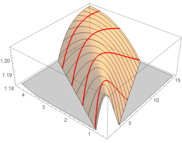
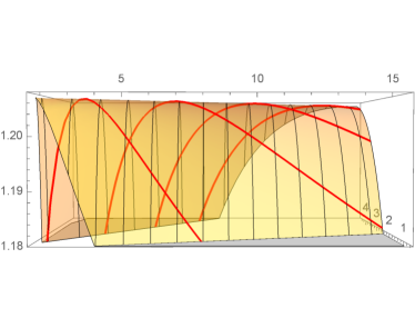
Figure 7: Graph of the function $(m,k)\mapsto\lambda_{m}^{\prime\prime}(k)=1+\frac{\sqrt{(2m-k)k}-k}{2m}$ showing the worst-case performance ratio with $m$ machines and $k$ long jobs

shows the function $(m,k)\mapsto\lambda_{m}^{\prime\prime}(k)$ with marked (thick) lines for integral values of $k$. One can also see the concave dependence on $k$ (thin lines). ∎

This concludes the proof of Theorem 5. In Figure 2 the graph of the function $m\mapsto\lambda_{m}(x_{m},0,k_{m})$, whose values at integral $m$ are exactly the worst-case approximation ratios for instances with $m$ machines, is depicted. The jumps and kinks occur when the number $k_{m}$ of long jobs in the worst-case instance changes. By taking the limit for $m\to\infty$, we obtain alternative proof of the performance ratio $\tfrac{1}{2}(1+\sqrt{2})$ by Kawaguchi and Kyan [14], avoiding the somewhat complicated transformation and case distinction in the proof of Lemma 3 and Schwiegelshohn’s proof [20]. For increasing $m$ the tight performance ratio converges quite quickly to $\tfrac{1}{2}(1+\sqrt{2})$: the difference lies in $O(1/m^{2})$. By plugging in the machine-dependent performance ratio into Theorem 1, we obtain the following performance ratio for the WSEPT rule.

Corollary 4.

For instances of the problem $P|\bm{p}_{j}\sim\mathrm{stoch}|\mathrm{E}[\sum w_{j}\bm{C}_{j}]$ with $m$ machines the WSEPT rule has performance ratio

$$1+\frac{1}{2}\cdot\frac{\sqrt{(2m-k_{m})k_{m}}-k_{m}}{m}(1+\Delta).$$

This bound is better than the bound of Corollary 3 only if $m$ and $\Delta$ both are small. Even for two machines, it is outdone for large $\Delta$ (see Figure 8).

Figure 8: Bound on WSEPT’s performance ratio for two machines

5 Open problem

For every fixed value of $\Delta$, one obtains the machine-independent performance ratio of $1+\tfrac{1}{2}(1+\min\{2,\sqrt{2+2\Delta}\})^{-1}(1+\Delta)$ for instances with squared coefficient of variation bounded by $\Delta$. On the other hand, for every fixed $m$ our performance bound tends to infinity when $\Delta$ goes to infinity, so that it does not imply a constant performance ratio (independent of $\Delta$) for instances with a constant number of machines. As far as the authors know, the question if such a $\Delta$-independent constant performance ratio of WSEPT for a fixed number of machines exists is still open. The examples of Cheung et al. [3] and of Im et al. [11] only show that no constant performance ratio can be given when $\Delta$ and $m$ are allowed to go simultaneously to infinity.

References

- [1] A. Avidor, Y. Azar, and J. Sgall. Ancient and new algorithms for load balancing in the norm. Algorithmica, 29(3):422–441, Mar. 2001.
- [2] C. Chekuri, R. Motwani, B. Natarajan, and C. Stein. Approximation techniques for average completion time scheduling. SIAM Journal on Computing, 31(1):146–166, Jan. 2001.
- [3] W. C. Cheung, F. Fischer, J. Matuschke, and N. Megow. A gap example for the WSEPT policy. Cited as personal communication in Uetz: MDS Autumn School Approximation Algorithms for Stochastic Optimization, 2014.
- [4] W. L. Eastman, S. Even, and I. M. Isaacs. Bounds for the optimal scheduling of jobs on processors. Management Science, 11(2):268–279, Nov. 1964.
- [5] M. X. Goemans. Improved approximation algorithms for scheduling with release dates. In M. Saks, editor, Proceedings of the Eighth Annual ACM-SIAM Symposium on Discrete Algorithms, pages 591–598. Society for Industrial and Applied Mathematics, 1997.
- [6] M. X. Goemans, M. Queyranne, A. S. Schulz, M. Skutella, and Y. Wang. Single machine scheduling with release dates. SIAM Journal on Discrete Mathematics, 15(2):165–192, 2002.
- [7] M. X. Goemans and D. P. Williamson. Two-dimensional Gantt charts and a scheduling algorithm of Lawler. SIAM Journal on Discrete Mathematics, 13(3):281–294, May 2000.
- [8] R. L. Graham, E. L. Lawler, J. K. Lenstra, and A. H. G. Rinnooy Kan. Optimization and approximation in deterministic sequencing and scheduling: a survey. In P. L. Hammer, E. L. Johnson, and B. H. Korte, editors, Discrete Optimization II, volume 5 of Annals of Discrete Mathematics, pages 287–326. Elsevier, 1979.
- [9] V. Gupta, B. Moseley, M. Uetz, and Q. Xie. Stochastic online scheduling on unrelated machines. In F. Eisenbrand and J. Koenemann, editors, Integer Programming and Combinatorial Optimization: 19th International Conference, Proceedings, pages 228–240, Cham, 2017. Springer International Publishing, arXiv:1703.01634.
- [10] L. A. Hall, D. B. Shmoys, and J. Wein. Scheduling to minimize average completion time: Off-line and on-line algorithms. In E. Tardos, editor, Proceedings of the Seventh Annual ACM-SIAM Symposium on Discrete Algorithms, pages 142–151, Philadelphia, PA, USA, 1996. Society for Industrial and Applied Mathematics.
- [11] S. Im, B. Moseley, and K. Pruhs. Stochastic scheduling of heavy-tailed jobs. In E. W. Mayr and N. Ollinger, editors, 32nd International Symposium on Theoretical Aspects of Computer Science, volume 30 of Leibniz International Proceedings in Informatics (LIPIcs), pages 474–486. Schloss Dagstuhl–Leibniz-Zentrum fuer Informatik, 2015.
- [12] C. Jagtenberg, U. Schwiegelshohn, and M. Uetz. Analysis of Smith’s rule in stochastic machine scheduling. Operations Research Letters, 41(6):570–575, Nov. 2013.
- [13] C. Kalaitzis, O. Svensson, and J. Tarnawski. Unrelated machine scheduling of jobs with uniform Smith ratios. In P. N. Klein, editor, Proceedings of the Twenty-Eighth Annual ACM-SIAM Symposium on Discrete Algorithms, pages 2654–2669, Philadelphia, PA, USA, 2017. Society for Industrial and Applied Mathematics, arXiv:1607.07631.
- [14] T. Kawaguchi and S. Kyan. Worst case bound of an LRF schedule for the mean weighted flow-time problem. SIAM Journal on Computing, 15(4):1119–1129, Nov. 1986.
- [15] N. Megow, M. Uetz, and T. Vredeveld. Models and algorithms for stochastic online scheduling. Mathematics of Operations Research, 31(3):513–525, Aug. 2006.
- [16] R. H. Möhring, F. J. Radermacher, and G. Weiss. Stochastic scheduling problems I — General strategies. Zeitschrift für Operations Research, 28(7):193–260, Nov. 1984.
- [17] R. H. Möhring, A. S. Schulz, and M. Uetz. Approximation in stochastic scheduling: The power of LP-based priority policies. Journal of the ACM, 46(6):924–942, Nov. 1999.
- [18] M. H. Rothkopf. Scheduling with random service times. Management Science, 12(9):707–713, May 1966.
- [19] A. S. Schulz. Stochastic online scheduling revisited. In B. Yang, D.-Z. Du, and C. A. Wang, editors, Combinatorial Optimization and Applications: Second International Conference. Proceedings, pages 448–457, Berlin, Heidelberg, 2008. Springer.
- [20] U. Schwiegelshohn. An alternative proof of the Kawaguchi–Kyan bound for the largest-ratio-first rule. Operations Research Letters, 39(4):255–259, July 2011.
- [21] M. Skutella. A 2.542-approximation for precedence constrained single machine scheduling with release dates and total weighted completion time objective. Operations Research Letters, 44(5):676–679, Sept. 2016, arXiv:1603.04690.
- [22] M. Skutella, M. Sviridenko, and M. Uetz. Unrelated machine scheduling with stochastic processing times. Mathematics of Operations Research, 41(3):851–864, Aug. 2016.
- [23] M. Skutella and G. J. Woeginger. A PTAS for minimizing the total weighted completion time on identical parallel machines. Mathematics of Operations Research, 25(1):63–75, Feb. 2000.
- [24] W. E. Smith. Various optimizers for single-stage production. Naval Research Logistics Quarterly, 3(1-2):59–66, Mar. 1956.
- [25] R. R. Weber, P. Varaiya, and J. Walrand. Scheduling jobs with stochastically ordered processing times on parallel machines to minimize expected flowtime. Journal of Applied Probability, 23(3):841–847, Sept. 1986.
- [26] G. Weiss. Approximation results in parallel machnies stochastic scheduling. Annals of Operations Research, 26(1):195–242, Dec. 1990.
- [27] G. Weiss. Turnpike optimality of Smith’s rule in parallel machines stochastic scheduling. Mathematics of Operations Research, 17(2):255–270, May 1992.