Effect of low anisotropy on cosmological models by using supernova data
Abstract
Abstract
pacs:
95.36.+x, 95.35.+dBy using the supernovae type Ia data we study influence of the anisotropy (although low) on the evolution of the universe and compare CDM model with 6 representative parametrizations of the recent Hubble expansion history . To compare these models we use the the maximum likelihood method for find that the best fit dynamical and obtained from the SNIa dataset. We have performed a comparative analysis of two SNIa datasets such as, the 194 SNIa
() and the most recent Supernova Legacy Survey (SNLS) dataset (238 data points ). In particular we find the best fit value of CDM model , with 194 SNIa and , with 238 SNLS high redshift type Ia Supernovae. The analysis shows that by considering the anisotropy, it leads to more best fit parameters in all models (except of SCDM) with SNIa data.
We also use two statistical tests such as the usual and p-test to compare different dark energy models. According to
both statistical tests and considering anisotropy, the CDM model that is providing the best fit to CDM of FRW model. An even better fit
would result with an optimization of the data using effects of anisotropy from the beginning.
keywords: Anisotropic universe, Dark energy, Supernovae type Ia, Luminosity distance
I Introductions
It is well known that the universe is currently undergoing accelerated cosmological expansion. Scientific observation shows that the accelerated expansion comes from supernova Type Ia (SNIa) apparent magnitude measurements as
a function of redshift 1 ; 2 ; 3 , cosmic microwave background (CMB) anisotropy data 4 ; 5 ; 6 combined with low estimates
of the cosmological mass density 7 , and baryon acoustic oscillation (BAO) peak length scale estimates 8 ; 9 .
Based on the years of analyzing the first year Wilkinson Microwave Anisotropy Probe (WMAP) data the observational results are formed 10 ; 11 .
By the introduction of a nonvanishing cosmological constant, the accelerated expansion is taken into account , where observations suggest a value of
12 in standard cosmology. The role of this cosmological constant is a non-clustering energy form, generally referred to dark energy (DE). According to the observations and standard particle physics theory, standard cosmology, including a universe filled by a cosmological constant along with the cold dark matter (CDM) and baryonic matters 13 . The simplest extension to is the DE with a constant , of which the corresponding cosmological model is the so-called CDM model, and a slowly rolling DE scalar field with an inverse power-law potential (CDM model) 14a ; 14 . Also a scalar field plays the role of DE, in the CDM scenario, as far as while spatial curvature is allowed to be non-zero in the CDM case, we consider a spatially-flat cosmological model, in the CDM and CDM cases. Different types of DE models have been reviewed previously such as quintessence 14 ; 15 ; 16 ; 17 ; 18 ; 19 ; 19a , phantom 20 ; 21 ; 22 , K-essence 23 ; 24 ; 25 and etc. In addition, the Chaplygin gas (CG) 26 ; 27 ; 28 and generalized Chaplygin gas (GCG) are considered extensively as an interaction between DE and dark matter (DM) 29 ; 30 ; 31 ; 32 . So far, from observations of high redshift SNIa, there is a tremendous amount of activity going on in trying to determine the equation of state and other cosmological parameters 33 ; 34 ; 35 ; 36 ; 37 ; 38 ; 38a . The most important way to measure the history of the cosmic expansion, is measurement of the luminocity distance relation. Since SNIa data measures the luminosity distance redshift relationship, it
provides a purely kinematic record of the expansion history of the universe. By using SNIa data without assuming the nature and evolution of the DE, probing the evolution of the Hubble parameter or the deceleration parameter is possible 39 ; 40 . These result are based on fitting a Friedman-Robertson-Walker (FRW) type geometry, together with the corresponding cosmology, to the existing astronomical data.
It is natural to assume that the geometry at very early epoch more general than just the isotropic and homogeneous FRW. Although on large scale at present, the universe seems homogeneous and isotropic, to guarantee of the isotropy there is no observational data in an era prior to the recombination. In fact, it is possible to begin with an
anisotropic universe which isotropizes during its evolution. Jaffe et al. 41 research’s show that removing a Bianchi component from the WMAP data can account for several large-angle anomalies leaving the universe to be isotropic. Therefore regardless of the inflation, in cosmological models, the universe may have achieved a slight anisotropic geometry. The Bianchi universe models 42 are spatially homogeneous anisotropic cosmological models.
From observational data, several strong limits on anisotropic models are investigated 43 ; 44 ; 44a . Sharif and Saleem 44b studied warm inflation for the Bianchi type I (BI) model and showed that this model is consistent with observational data. Also, Sharif and Siddiqa 44c examined
effects of viscosity on anisotropic universe in modified gravity and observed that bulk viscosity enhances expansion of the universe.
Recently, Hossienkhani et al. 45 discussed the effects of the
anisotropy on the evolutionary behavior DE models and compare with the results of the standard FRW, CDM and CDM
models. Also, they shown that the anisotropy is a non-zero value at the present time although it is approaching zero, i.e. the anisotropy
will be very low after inflation. Hence, the effects of anisotropy can be investigated in the context of DE and DM models although it is low. In this paper the usefulness of anisotropy effect to assess the parameters of several popular DE models investigate
and compare our results with the inference made
using luminosity distances measured with SNIa.
The paper is organized as follows. In the next section, we present the field equations for the BI universe and derive the cosmological evolution of
the equation of state parameter and the deceleration parameter for several DE models. In section III we fit the derived Hubble parameter to the
SNIa dataset and obtain constraints for the various DE models in a flat BI model.
In section IV we present our results for the best fits and discuss their implications and common features. This analysis is repeated with data obtained from
observationally allowed thawing models even though this class of models has small allowed deviations from CDM model.
In section V we briefly summarize the contents of the SNLS sample and describe the light-curve fitting method and the model parameters (including those associated with the data) that are to be estimated. The last section is devoted to summary and conclusions.
II Anisotropy effects and cosmological analysis using SNIa data
In our analysis, the most typical and commonly used current observations are chosen, i.e., the type Ia supernovae (SNIa), and direct measurement of the luminocity distance. In other words, SNIa can be calibrated to be good cosmological standard candles, with small dispersions in their peak luminocity 46 . We begin with a brief outline of the method of our analysis of the supernova data. The luminosity distance to an object at redshift is such that
| (1) |
where is the comoving distance and the relation between the light ray geodesic and the comoving distance in in a flat universe is , where is the scale factor. The apparent magnitude of the source with an absolute magnitude is related to the luminosity distance with 47 ; 48
| (2) |
The absolute magnitude after correcting for supernova light curve width - luminosity correlation 2 ; 49 . After applying the above correction, , and hence , is believed to be constant for all SNIa. In the case of SNIa, the first step is almost trivial since the textbook expression for reads
| (3) |
where is the Hubble parameter as a function of redshift and terms of arbitrary parameters. The predicted can be compared with the observed to test the consistency of the theoretical model with observations. In this paper, we would like to use both the maximum likelihood estimation (MLE) 50 and the SNIa of the dataset compiled in 47 . So, we can find the goodness of fit to the corresponding observed () coming from the SNIa data 47 . The goodness of fit corresponding to any slope is determined by the probability distribution of i.e. 50
| (4) |
where is a normalization constant. We also call this measure “p-test” and it will be used in what follows to compare the quality of the parametrizations considered. The theoretical model parameters are determined by minimizing the quantity 40a
| (5) |
where for SNIa, is a free parameter representing the difference between the actual , and are the redshift uncertainty and errors of the data and respectively. These errors are assumed to be Gaussian and uncorrelated. In the case of , we assumed no prior constraint on , which is just an unknown constant with a value between and . In this case, we integrated the probabilities on and therefore worked with a defined by
| (6) |
where
| (7) | |||
| (8) | |||
| (9) |
with . The steps we followed for the usual minimization of Eq. (5) in terms of its parameters are described in detail in 50a ; 51 ; 52 . This approach assumes that there is some theoretical model available, given in the form of , which is to be compared against the data. As a result of the analysis, the best-fit parameter values and the corresponding and error bars are obtained. The error on is determined by the relation 50
| (10) |
where the best fit value of is given by the value that minimizes . From Eq. (10) is in the range with 68% probability for , where is the number of free model parameters. Also the error with 95.4% range which that is determined by
.
To evaluate the influence of both the global expansion and the line of sight conditions on light propagation we
examine an anisotropic accurate solution of the Einstein field equations. The BI cosmology has different expansion rates along the three orthogonal spatial directions, given by the metric
| (11) |
where , and are the scale factors which describe the anisotropy of the model and the average expansion scale factor . It reduces to the FRW case when . Defining the time-like hypersurface-orthogonal vector , we can define the average Hubble scalar, , and the shear, , as follows:
| (12) |
Einstein’s field equations for the BI metric is given in (11) which lead to the following system of equations 45 ; 53
| (13) | |||
| (14) | |||
| (15) |
where and are the energy density and pressure of DE, respectively. We also define , here is Newton’s gravitational constant and will use the unit . One can rewrite Eq. (13) in the form
| (16) |
where
| (17) | |||||
| (18) |
where is the redshift, , is
probably the current fractional density due to so-called anisotropy
and is the current fractional density of non-relativistic
matter.
Eq. (16) shows that the sum of the energy density parameters approaches at late times if the shear
tensor tend zero. Hence, at the late times the universe becomes flat, i.e. for sufficiently large time, this model
predicts that the anisotropy of the universe will damp out and universe will become isotropic.
The DE is usually described by an equation of state parameter (EoS) . Using Eqs. (13) and (14) we can obtain the expression for EoS parameter
| (19) |
Independently of its physical origin, the parameter is an observable derived from and is usually used to compare theoretical model predictions with observations. When the anisotropy density goes to zero, i.e. , and (i.e. spatially flat FRW universe), the EoS parameter is reduced to that of the 40a ; 51 ; 54 . Also, the acceleration of the universe can be quantified through a cosmological function known as the deceleration parameter , equivalently
| (20) |
where describes an accelerating universe, whereas for a universe which is decelerating phase.
III Likelihood analysis and comparison of DE models using SNIa dataset
We will consider five representative parametrizations and minimize the of Eqs. (5) with respect to
model parameters. We compare the best fit parametrizations obtained with SNIa dataset. Besides a measure of the quality of fit may be defined in analogy
to the likelihood for comparison of DE models to be used with a given set of data. Refs. 55 ; 56 motivated by the high likelihood of the phantom divide
line crossing indicated by the Gold datasets 38 ; 57 to examine theoretical models that predict such crossing. Note that an additional uncertainty from the redshift
dispersion due to peculiar velocity must be added to the uncertainty of each SNIa data point. So, one must propagate
into an additional uncertainty in the luminosity distance.
Let us start our analysis with the flat BI model where , with two free parameters . We have also chosen the parameter from recent Planck data observed and WMAP-9 data as 58 .
Other best fit values determined by Strong gravitational lensing (SGL) and CBS (CMB+BAO+SNIa) data are , 59 , and the 5-year Supernova Legacy Survey (SNLS) data is 60 . We first show preliminary results for which the matter
density and the Hubble parameter are fixed at a constant values of 40 ; 61 and 62 . The fact that
we have fixed instead of marginalizing over it could
have artificially decreased somewhat the error bars of the
parameters.
The first and simplest model to study is matter dominated SCDM which is defined in an anisotropic universe as follows:
| (21) |
We recall that the above equation is obtained from the first BI equation i.e. Eq. (13).
The value of that minimize the of Eq. (5) (with given by Eq. (21)) obtained by SNIa dataset. So we find
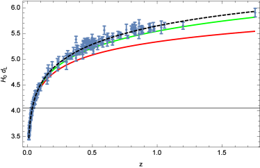
which results , where is degrees of freedom111The value of for the model equals the number of observational data points minus the number of parameters.. Because the value of is larger than 1. Therefore, SCDM is not suitable for SNIa data as shown in Fig. 1 (red line).
One of the simplest DE model is the cosmological constant with the EoS parameter . Although is the simplest model, it suffers from severe theoretical and conceptual problems, such as the fine-tuning and the cosmic coincidence problems 48 . In the CDM model Hubble’s parameter is given by
| (22) |
Using Eq. (5) we get the best fit value of CDM model parameter is with , and the reduced value is . While in the FRW model, the value of is equal to 40a ; 63 . This shows that the CDM model with considering the effects of the anisotropy, it taken to be the best-fit ones from SNIa data. In the case of errors on the value of and by solving Eq. (10) we get
| (23) |
In the following, we recall for comparison different DE models, we consider with .
Figure 1 illustrates the observational values of the luminosity distance versus redshift together with the theoretical curves derived from (3).
The luminosity distance becomes larger when the cosmological constant is present and it provides a good fit to
the data unlike to the case of SCDM model. In addition, Fig. 1 shows that a matter dominated universe (SCDM) in a BI universe does not fit to the data. For the case of SCDM model, a best-fit value of obtained in refs. 40 ; 61 ; 64 is (isotropic universe).
In order to fit the model with current observational data, we consider five DE models in a flat BI in this section.
III.1 CDM model with the constant EoS parameter 57
The next step is to allow for deviations from the simple case, introducing a component with an arbitrary, constant value for the EoS parameter. The accelerated expansion is achieved when 14 . The Hubble parameter evolves according to the BI equation, which for is
| (24) |
For we recover the limiting form Eq. (22). Observational constraints on the CDM model have been derived from many different data sets, hence it provides a useful basis for comparing the discriminative power of different data. The currently preferred values of is given by: 65 , 6 and from the CMB and baryon acoustic oscillation (BAO) 66 . Equation (24) depends on two parameters, and . Since the depends on two parameters. We use Eq. (5) to produce and analyze the MLE. In particular, for the case of we obtain
| (25) |
and the best fit value with the errors is
| (26) |
Also, for the value of , we find and . This indicates that the minimization of CDM model, exactly the goodness-of-fit of the CDM model for the same data.
III.2 Quiessence- () model 40a
In this subsection we obtain a combination of cosmological constant with quiessence (). Then we examine the effects of anisotropy on the cosmological implications of this model, and using the SNIa data we probe observational constraints. The corresponding form of for the model in BI universe is
| (27) |
If we set and fit the 194 SNIa data, we get the best fitting values as follows:
| (28) |
Considering the error bars we find that and . Based on Eqs. (19) and (20), the confidence levels of the best fit and calculated by using the MLE for Eq. (5) are plotted in Fig. 2 with and . From Fig. 2a, it is easy to see
that the can not cross , which corresponds to the quintessence phase. On the other hand, at behaves like the cosmological constant, i.e. . In conclusion, when our analysis is compared with that of ref. 40a , it is seen that the EoS parameter
in the of FRW model has a lower slope than the EoS parameter in of BI model, that this reflects that
anisotropy effects causes accelerating expansion so rapidly. For a better insight, it was also seen that the EoS parameter passes from the dominant matter to the DE region in the range of 40a , while it happens in the range of in the present work (see Fig. 1a).
From Fig. 2b, we find out the
deceleration parameter is positive at large , which indicates the earlier decelerating phase of the universe. Furthermore, we can see that the best fit values of transition redshift and current deceleration parameter with confidence levels are and , which is consistent with the observations of 67 . For comparison the combined analysis of SNe+CMB data with the CDM model gives the range and the present value of the deceleration parameter 68 (assuming ) and the matter dominated regime
() is reached by . Recent studies have constructed takeing into account that the strongest evidence of accelerations happens at redshift of . In order to do so, the researcher have set to reconstruct it and after that they have obtained by fitting this model to the observational data 69 . Also it found that for within the level.
Notice that the errors in Fig. 2 increase with redshift.
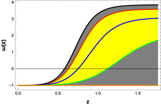
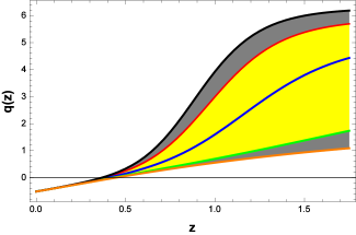
In the following, we follow the process of subsection A and we introduce other DE models. Then we obtain the form and the parameters requiring fitting. Finally, we figure out and minimize with respect to these parameters by considering . In order to simplify and avoid confusion we only show the best fit curves without the corresponding and confidence limits.
III.3 Linear parametrization with 70 ; 71 ; 72 ; 73 ; 74
In order to discriminate between a cosmological constant and dynamical DE we use the DE EoS parameter parametrization 70 ; 71 ; 72 ; 73 ; 74
| (29) |
where and are the constant. This model is interesting because it is described by simple field equations. The cosmological constant (CDM) corresponds to and , the case of constant EoS parameter (CDM) corresponds to and , while the general case of time-evolving DE corresponds to . The DE density for this case is given by
| (30) |
In this case Eq. (13) gives the Hubble parameter
| (31) |
We can then constrain the two parameters and by using SNIa data. The results obtained with standard rulers turned out to correspond well with previous work by 75 , whose results were , . As far as standard candles are concerned, the result of joint analysis from WMAP+BAO+H0+SN given by 76 is , . The allowed confidence limits for (), derived from the joint analysis SNIa data are: and with .
III.4 Chaplygin gas and Generalized Chaplygin gas
The expansion rate in the generalized Chaplygin gas (GCG) of BI model is governed by the equation
| (32) |
It is straightforward to show that this equation of motion reduces to the isotropic universe in the limiting case corresponding to 76a ; 77 ; 78 ; 79 . Also, for the case of 26 ; 27 ; 28 ; 40a ; 80 the model recovers the Chaplygin gas model (CG). Within the framework of BI, we study a model based on CG where our principal assumption is that the energy density and pressure are related by the following EoS
| (33) |
From Eq. (5) it can be seen that the GCG behaves like pressureless dust at early times and like a cosmological constant during very late times. In the following section, we will use the cosmic observations to constrain the GCG and CG models parameter . One can see that this constraint on parameter is more stringent than the results in refs. 81 ; 82 , where the constraint results for the GCG model parameters are and at confidence limits with the X-ray gas mass fractions of galaxy clusters and the dimensionless coordinate distance of SNe Ia and FRIIb radio galaxies 81 , and and at confidence limits with the 115 SNLS SNe Ia data and the SDSS baryonic acoustic oscillations peak 82 . We allow now more anisotropy in our model and consider the value for . In the case of GCG model the best fit values for and are and the resulting is showing that there is an improvement in the quality of fit. However, if we calculate the case of CG model for the best fit among the SNIa data (corresponding to a model with ) we find (the errors are at the level).
IV Comparison between the present models
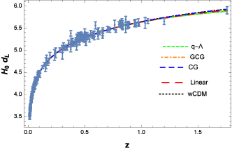
Table I: A comparison of the models used in the work. In all cases we have assumed .
Model
p-test
Best Fit Parameters
CDM
SCDM
CDM
q-
,
Linear
,
GCG
CG
In this section, we choose several popular DE models and estimate their best fitted
parameters using the SNIa data. We also examine consistency of our findings with
other independent results from the literature and we apply the effects of anisotropy on the p-test to rank 6 representative parametrizations of . The comparison of the parametrizations considered is shown in Table I. In all cases we have assumed priors corresponding to flatness and and . It can be seen that the linear parametrization model has the smallest . Also the per degree of freedom for
the best-fit for the different cases is given in Table I.
Figure 3 shows the luminosity distance measured by the SNIa compared to various possible models of Table I, which strongly favours a DE model.
It shows that the effect of anisotropy on is nearly identical for the set of models as individual curves can hardly be distinguished.
In the next step, we examine the EoS and deceleration parameter for the DE models studied in the previous section. In Fig. 4 we plot the best fit and for 5 representative parametrizations of Table I. Among the models, the linear parametrization and CDM models that are providing the best
fit to the EoS parameter exhibit crossings of the divide line (see Fig. 4a). Fig. 4b shows that the universe transits from a matter dominated epoch at early times to the acceleration phase in the present time, as expected. In Table II, we list the results of , and for the current universe ().
We have also found that the constraints obtained on the parameter
values by the SNIa datasets. The Gaussian distribution is the most important distribution in statistics, because it is so ubiquitous
(so “normal”), appearing in many different experimental settings, and because many other distributions approach the normal distribution as soon as they become “messy”. The full probability distribution, for example, converges to the normal distribution for a large numbers of data samples.
The central limit theorem of probability theory tells us that a sum of identically distributed independent variables has, in the limit, a normal distribution.
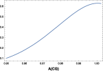
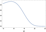
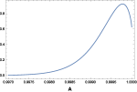
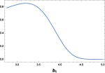
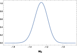
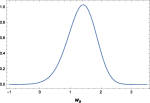
It is seen from the likelihood plots (Fig. 5) that the likelihood functions are well fitted to a Gaussian distribution function for each
dataset. The corresponding constraints on model parameters are summarized in Table I.
Finally, the reduced form of compared to CDM model determined as
| (34) |
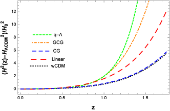
where is the reduced form of and . In the Fig. 6, we plot the deviation of the squared Hubble parameter from CDM over redshift for the best fit. From this figure, we see that expansion is faster when DE is model as compared to other DE models. But in range of , the curves are coincide, that is the effect of anisotropy parameter density is constant.
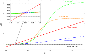
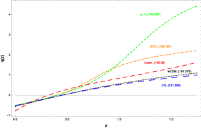
Table II: The results of , and for five DE models used in the work.
Model
CDM
Linear
q-
GCG
CG


V Light curve parameters of SNLS
To derive the brightness, light-curve shape and SN color estimates required for the cosmological analysis, the time sequence of photometric measurements for each SN was fit using a SN light-curve model. Guy et al. 83 presents the light curves of the SNLS SNe Ia themselves, together with a comparison of SN light curve fitting techniques, color laws, systematics and parameterizations. Conley et al. 83a compared the performances of different light-curve fitters while also introducing their own empirical fitter, SiFTO, and concluded that SALT2 along with SiFTO perform better than both SALT (which is conceptually different from its successor SALT2) and MLCS2k2 (Jha et al. 83b ) when judged by the scatter around the best-fit luminosity-distance relationship. We parameterize the SN Ia light curves for distance estimation using the combined results from updated version of light curve fitter SiFTO. It technique provide an estimate of the SN peak rest-frame B-band apparent magnitude at the epoch of maximum light in that filter, a measure of the SN light curve shape, and an estimate of the SN optical B-V color (). Guy et al. 83 discarded from the SNLS catalog 252 SNe with a peak rest-frame . This cut, applied to both SALT2 and SiFTO samples, discards 11 SNe. There are also three SNe whose peak magnitudes could not be obtained with SiFTO due to a lack of observations in the and bands. Hence, that leaves SNLS SNe. From the fits to the light-curves, we computed a rest-frame-B magnitude, which, for perfect standard candles, should vary with redshift according to the luminosity distance. This rest-frame-B magnitude refers to observed brightness, and therefore does not account for brighter-slower and brighterbluer correlations 84 . The observed distance modulus of each SN is given by 83 ; 84 ; 85
| (35) |
where is the observed peak magnitude in rest frame B band, is the stretch (a measure of light-curve shape), corresponds to the supernova color at maximum brightness. Notice that , and are nuisance parameters in the distance estimate, which should be fitted simultaneously with the cosmological parameters. The theoretical model parameters are determined by minimizing the quantity 83 ; 84 ; 85
| (36) |
where is given by Eq. (2), for the joint light-curve analysis (JLA) SNIa, and are the errors due to flux uncertainties, intrinsic dispersion of SNIa absolute magnitude. The SN-specific dispersion is defined by
| (37) |
Where , and are the standard errors of the peak magnitude and light-curve parameters of the i-th SN. The term comes from the covariances among and likewise depends quadratically on and . For the case of , we perform a first fit with an initial value (typically 0.15 mag.), and then calculate the required to obtain a reduced . We then refit with this more accurate value. We fit 6 cosmologies to the data that was introduced in Table I. To find the best-fit coefficients , and and the cosmological parameters that define the fitted model, we use MLE techniques, which is based on the maximization of a joint likelihood function. Using the MLE approach, we find that the best-fit curvature parameter using the JLA SNe Ia data and the considering effect of anisotropy, the optimized nuisance parameters are , , , and with . In Figure 7 we show the (normalized) likelihood distribution for each parameter (, , , , ), according to the factor , and , contours for the joint distribution of each pair of parameters. For each parameter, the likelihood distribution is well approximated by a Gaussian, and the stated confidence interval is a 68% (i.e., ) interval for this Gaussian. The maximum value of the joint likelihood function for an anisotropic universe corresponds to . In conclusion, when our analysis is compared with that of ref. 85 , it is seen that the maximum value of the joint likelihood function in the CDM of FRW model has a bigger than the maximum value of the joint likelihood function in the CDM of BI model, that imply that anisotropy effects causes improves the data fitting in the CDM DE model. The resulting color and light-curve shape corrected peak B-band magnitudes for the various cosmological models are presented in Table III. The parameters , , and are nuisance parameters which are fitted simultaneously with the cosmological parameters. From Table III, it can be observed that the CDM DE model has the smallest .

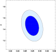

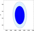
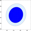

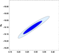
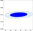
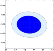

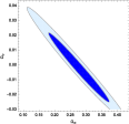
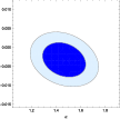
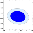
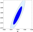

Table III: Best Fits for Different Cosmological Models for JLA SNe Ia.
Model
Other Best Fit Parameters
CDM
CDM
q-
Linear
GCG
CG
VI Conclusion
In this work, we have investigated the anisotropy effects on the various cosmological models, by using the two
SNIa datasets available in the work: the SNIa data by Tonry et al. and Barris et al. in the
redshift range and the most recent SNLS dataset (238 data points ). We have fitted these models using the MLE and compare our results with the inference made using luminosity distances measured with both SNIa data points. We have used representative
DE parametrizations to examine the consistency among the two datasets in constraining the corresponding parameter values.
Based on these properties, we have evaluated the quality of fit of several DE models
and it was compared the observed expansion rate with that predicted by the various models proposed in Table I.
In comparing the quality of fit we have used the value of and the p-test in BI models. We have reported the model independent reconstruction of the cosmic EoS and deceleration parameter of DE. Our main conclusions can be summarized as follows.
-
•
The first and simplest studied model was SCDM model and we found for it, by using the data from 194 SNIa 47 . Fig. 1 exhibits that applying anisotropy for the data fitting is not adequate for SCDM model.
-
•
Another simple model was the CDM model in which parameter is the free parameter. The best is equal to with and . We also showed that applying anisotropy on this model leads to the good fit using the SNIa data (see Fig. 1).
-
•
We found the best fitted parameter in CDM model by fixing is with . This result shows that the minimization of the CDM model improves the data fitting in CDM model in comparison with the CDM model. In other words, EoS parameter can cross the phantom divide line, if the CDM model is fitted using the data obtained from SNIa, and we found and at the first level of error.
-
•
In the -q model the best fitting parameter, for SNIa data and by considering anisotropy was and with . In this model, the EoS parameter cannot cross the phantom divide line, i.e. this model is in an agreement with the quintessence model. As Fig. 2 suggests, applying anisotropy leads to a faster accelerated expansion for the universe. We also found that the amount of at the current time is and the transition redshift is .
-
•
We obtained and with , by applying anisotropy to the linear model. Table I shows a better fitting in comparison to other two models. In this table the minimum amount of has been presented. Therefore, among the DE models studied in present work, we are interested in the linear model by using SNIa data. The EoS parameter can also cross phantom divide line in this model. We calculated the parameter and the transition redshift in this model and its results are and .
-
•
We have analyzed the currently available 194 supernova data points within the framework of the generalized Chaplygin gas and Chaplygin gas models. We have considered both, flat and non-isotropic cases, and found the best fit parameters in the generalized Chaplygin gas model are and with . The generalized Chaplygin gas model tends to be the CDM model in order to recover the standard cosmology at early times. In other words, our results show that the generalized Chaplygin gas model is almost the same as the CDM model than the Chaplygin gas model. It is easy to see that the best fit can not cross as it evolves with the redshift , and the present best fit value as shown in Fig. 4a. The transition redshift when the universe underwent the transition from deceleration to acceleration is found to be . We also find that the present deceleration parameter is (see Fig. 4b). But in the case of the Chaplygin gas model the best-fit values of parameter is with at the level. In Table II we present values of the EoS and deceleration parameters for generalized Chaplygin gas and Chaplygin gas model. It can be seen clearly that the generalized Chaplygin gas model is preferred of the Chaplygin gas model by SNIa data. The fact that the properties of the Chaplygin gas interpolate between those of SCDM and a CDM led to the hope that the Chaplygin gas might provide a conceptual framework for a unified model of DM and DE.
-
•
We also consider the light curve fitters for our analysis. It is intended to estimate three parameters (magnitude, shape and colour) that can be subsequently linearly combined to determine the luminosity distances of the SNe Ia. Unlike previous section, we have assumed prior corresponding to , this approach can thus adversely affect the validity of the fitting method and lead to compromised or misleading results. Therefore to counteract this problem, we does not require the prior on all parameters, fit by the SNLS dataset. Consider no prior of and the SN light-curve model, we re-optimize parameters by carrying out an MLE in any situation where the parameters include an unknown intrinsic dispersion. The commonly used method, which estimates the dispersion by requiring the reduced to equal unity, does not take into account all possible covariances among the parameters. We have found that, when the parameter optimization is handled via the joint likelihood function, DE models fit their individually optimized data very well. In the CDM model, the JLA sample provides a measurement of the reduced matter density parameter , which is in good agreement with the recent measurement from the JLA and lowz+SNLS 86 , SN-stat 87 and SNeIa+CMBShift 88 .
Finally, seven models and considering anisotropy on them were investigated. By comparing between Tables I and III, it was concluded that fitting the SNIa data and applying anisotropy, leads to an improvement of the SNIa data (except for the SCDM model). The best fit parameters in a CDM parametrization without a prior show interesting differences between the Tonry and Barris et al. and the JLA SNIa datasets. Thus, our study shows that the anisotropy effects on the CDM DE model is a very good fit to the latest JLA SNIa data.
References
- (1) A.G. Riess, A.V. Filippenko, P. Challis et al., Astron. J. 116, 1009 (1998).
- (2) S. Perlmutter, G. Aldering, G. Goldhaber et al., Astrophys. J. 517, 565 (1999).
- (3) R. Amanullah et al., Astrophys. J. 716, 712 (2010).
- (4) B. Ratra et al., Astrophys. J. 517, 549 (1999).
- (5) S. Podariu et al., Astrophys. J. 559, 9 (2001).
- (6) D.N. Spergel et al., Astrophys. J. Suppl. 148, 175 (2003).
- (7) G. Chen, B. Ratra, PASP 115, 1143 (2003).
- (8) D.J. Eisenstein et al., Astrophys. J. 633, 560 (2005).
- (9) Y. Wang, Mod. Phys. Lett. A 25, 3093 (2009).
- (10) E. Komatsu et al., Astrophys. J. Suppl. 180, 330 (2009).
- (11) D.N. Spergel et al., Astrophys. J. Suppl. 148, 175 (2003).
- (12) J. Beringer et al., Phys. Rev. D 86, 010001 (2012).
- (13) M. Hicken et al., Astrophys. J. 700, 1097 (2009).
- (14) P.J.E. Peebles, B. Ratra, Astrophys. J. 325, L17 (1988).
- (15) B. Ratra and P.J.E. Peebels, Phys. Rev. D 37, 3406 (1988).
- (16) C. Wetterich, Nucl. Phys B 302, 668 (1988).
- (17) S.M. Carroll, Phys. Rev. Lett. 81, 3067 (1998).
- (18) M. Tegmark et al., Phys. Rev. D 69, 103501 (2004).
- (19) H.V. Peiris et al., Astrophys. J. Suppl. Ser. 148, 213 (2003).
- (20) V. Sahni and L.M. Wang, Phys. Rev. D 62, 103517 (2000).
- (21) M. Khurshudyan, A. Pasqua, J. Sadeghi and H. Farahani, Chinese Phys. Lett. 32, 109501 (2015).
- (22) T. Chiba, T. Okabe, M. Yamaguchi, Phys. Rev. D 62, 023511 (2000).
- (23) R.R. Caldwell, Phys. Lett. B 545, 23 (2002).
- (24) R.R. Caldwell, M. Kamionkowski and N.N. Weinberg, Phys. Rev. Lett. 91, 071301 (2003).
- (25) C. Armendáriz-Picón, V. Mukhanov and P.J. Steinhardt, Phys. Rev. Lett. 85, 4438 (2000).
- (26) C. Armendáriz-Picón, V. Mukhanov and P.J. Steinhardt, Phys. Rev. D 63, 103510 (2001).
- (27) T. Chiba, T. Okabe and M. Yamaguchi, Phys. Rev. D 62, 023511 (2000).
- (28) A. Kamenshchik, U. Moschella and V. Pasquier, Phys. Lett. B 511, 265 (2001).
- (29) M.C. Bento, O. Bertolami and A.A. Sen, Phys. Rev. D 66, 043507 (2002).
- (30) V. Gorini, A. Kamenshchik, U. Moschella, Phys. Rev. D 67, 063509 (2003).
- (31) N. Bilic, G.B. Tupper and R.D. Viollier, Phys. Lett. B 535, 17 (2002).
- (32) O. Bertolami, A.A. Sen, S. Sen, P.T. Silva, MNRAS. 353, 329 (2004).
- (33) U. Debnath, A. Banerjee, S. Chakraborty, Class. Quant. Grav. 21, 5609 (2004).
- (34) M.C. Bento, O. Bertolami and A.A. Sen, Phys. Lett. B 575, 172 (2003).
- (35) Z.-H. Zhu, M.-K. Fujimoto and X.-T. He, A&A, 417, 833 (2004).
- (36) Y. Wang , M. Tegmark, Phys. Rev. Lett. 92, 241302 (2004).
- (37) Y.-G. Gong, X.-M. Chen, C.-K. Duan, Mod. Phys. Lett. A19, 1933 (2004).
- (38) Y.-G. Gong, C.-K. Duan, MNRAS. 352, 847 (2004).
- (39) J.S. Alcaniz, N. Pires, Phys. Rev. D 70, 047303 (2004).
- (40) Y. Wang, P. Mukherjee, ApJ 606, 654 (2004).
- (41) A. Pasqua, S. Chattopadhyay, Int. J. Theor. Phys. 53, 435 (2014).
- (42) M.S. Turner and A.G. Riess et al., Astrophys. J. 569, 18 (2002).
- (43) A.G. Riess Astrophys. J. 607, 665 (2004).
- (44) S. Nesseris and L. Perivolaropoulos, Phys. Rev. D 70, 043531 (2004).
- (45) T.R. Jaffe et al., ApJ 643, 616 (2006).
- (46) G.F.R. Ellis, Gen. Rel. Grav. 38, 1003 (2006).
- (47) M.Tirandari and Kh.Saaidi, Nuclear Physics B, 925, 403 (2017).
- (48) A. Bernui, B. Mota, M.J. Reboucas and R. Tavakol, Astron. Astrophys. 464, 479 (2007).
- (49) M. Ahlers and P. Mertsch, Nuclear Physics B, 94, 184 (2017).
- (50) M. Sharif and R. Saleem, Eur. Phys. J. C 74, 2738 (2014).
- (51) M. Sharif and A. Siddiqa, Commun. Theor. Phys. 69, 537 (2018).
- (52) H. Hossienkhani et al., Physics of the Dark Universe 18, 17 (2017).
- (53) A.G. Riess, W.H. Press and P.R. Kirshner, ApJ 438, L17 (1995); M.M. Phillips, ApJ 413, L105 (1993).
- (54) J.L. Tonry, B.P. Schmidt, B. Barris et al., ApJ 594, 1 (2003); B.J. Barris, J. Tonry, S. Blondin et al., ApJ 602, 571 (2004).
- (55) V. Sahni and A.A. Starobinsky, Int. J. Mod. Phys. D 9, 373 (2000); T. Padmanabhan, Phys. Rept. 380, 235 (2003).
- (56) M.M. Phillips, P. Lira, N.B. Suntzeff et al., Astron. J. 118, 1766 (1999); A.G. Riess, W.H. Press and R.P. Kirshner, ApJ 473, 88 (1996).
- (57) W.H. Press et al., ‘Numerical Recipes’, Cambridge University Press (1994).
- (58) E.Di Pietro and J.F. Claeskens, Mon. Not. Roy. Astron. Soc. 341, 1299 (2003).
- (59) S. Nesseris and L. Perivolaropoulos, JCAP 0701, 018 (2007).
- (60) S. Nesseris and L. Perivolaropoulos, Phys. Rev. D 72, 123519 (2005).
- (61) H. Hossienkhani, et al., Theoretical and Mathematical Physics, 194, 415 (2018); H. Hossienkhani, et al., Eur. Phys. J. Plus 133, 30 (2018); H. Hossienkhani, et al., Commun. Theor. Phys. 69, 467 (2018); H. Hossienkhani and A. Pasqua, Astrophys Space. Sci. 349, 39 (2014).
- (62) T.D. Saini, S. Raychaudhury, V. Sahni and A.A. Starobinsky, Phys. Rev. Lett. 85, 1162 (2000); D. Huterer and M.S. Turner, Phys. Rev. D 64, 123527 (2001).
- (63) L. Perivolaropoulos, JCAP 10, 001 (2005).
- (64) B. Feng, X.L. Wang and X.M. Zhang, Phys. Lett. B 607, 35 (2005).
- (65) U. Alam, V. Sahni and A.A. Starobinsky, JCAP 0406, 008 (2004); U. Alam, V. Sahni, T.D. Saini and A.A. Starobinsky, MNRAS. 354, 275 (2004).
- (66) J.F. Zhang, L.A. Zhao, X. Zhang, Sci. China Phys. Mech. Astron. 57, 387 (2014).
- (67) J. Cui, Y. Xu, J. Zhang, et al., Sci. China Phys. Mech. Astron. 58, 110402 (2015).
- (68) P. Astier et al., Astron. Astrophys. 447, 31 (2006).
- (69) T.R. Choudhury and T. Padmanabhan, Astron. Astrophys. 429, 807 (2005).
- (70) D.N. Spergel, R. Bean, O. Doré et al., Astrophys. J. Suppl. 170, 377 (2007).
- (71) J. Lu, Y. Gui and Li. Xu, Eur. Phys. J. C 63, 349 (2009).
- (72) E.J. Copeland, M. Sami and S. Tsujikawa, Int. J. Mod. Phys. D 15, 1753 (2006).
- (73) T.M. Davis, E. Mortsell, J. Sollerman et al., Astrophys. J 666, 716 (2007).
- (74) P.A.R. Ade et al., Planck Collaboration, A&A, 571, A16 (2014).
- (75) R.A. Daly et al., J. Astrophys 677, 1 (2008).
- (76) Y.G. Gong and A. Wang. Phys. Lett. B 652, 63 (2007).
- (77) Y.G. Gong and A. Wang. Phys. Rev. D 75, 043520 (2006); Y.G. Gong and A. Wang. Phys. Rev. D 73, 083506 (2006).
- (78) J. Weller and A. Albrecht, Phys. Rev. D 65, 103512 (2002).
- (79) I. Maor, R. Brustein, J. McMahon and P.J. Steinhardt, Phys. Rev. D 65, 123003 (2002).
- (80) M. Goliath et al., A&A, 380, 6 (2001).
- (81) V. Barger and D. Marfatia, Phys. Lett. B 498, 67 (2001).
- (82) J. Weller and A. Albrecht, Phys. Rev. Lett. 86, 1939 (2001).
- (83) M. Biesiada, et al., RAA, 11, 641 (2011).
- (84) E. Komatsu, et al., APJs, 192, 581 (2011).
- (85) V. Sahni, Lect. Notes Phys. 653, 141 (2004).
- (86) J.S. Alcaniz, D. Jain and A. Dev, Phys. Rev. D 67, 043514 (2003).
- (87) P.P. Avelino, L.M.G. Beca, J.P.M. de Carvalho and C.J.A. Martins, JCAP 0309, 002 (2003).
- (88) M.C. Bento, O. Bertolami and A.A. Sen, Gen. Rel. Grav. 35, 2063 (2003); M.C. Bento, O. Bertolami and A.A. Sen, Phys. Rev. D 67, 063003 (2003).
- (89) J.C. Fabris, S.V.B. Goncalves and P.E.d. Souza, arXiv:astro-ph/0207430.
- (90) Z.H. Zhu, Astron. Astrophys. 423, 421 (2004).
- (91) P.X. Wu and H.W. Yu, Phys. Lett. B 644, 16 (2007).
- (92) J. Guy, M. Sullivan, A. Conley, et al., A&A, 523, A7 (2010).
- (93) A. Conley, et al., ApJ, 681, 482 (2008).
- (94) S. Jha, A.G. Riess and R.P. Kirshner, ApJ, 659, 122 (2007).
- (95) J. Guy, P. Astier, S. Nobili, N. Regnault and R. Pain, A&A, 443, 781 (2005).
- (96) J.J. Wei, X.F. Wu, F. Melia and R.S. Maier, AJ, 149, 102 (2015).
- (97) M. Betoule, R. Kessler, J. Guy, et al., A&A, 568, A22 (2014).
- (98) D.M. Scolnic, D.O. Jones, A. Rest, et al., ApJ, 859, 101 (2018).
- (99) A. Mukherjee, and N. Banerjee, Eur. Phys. J. Plus 130, 201 (2015).