Comparing the Forecasting Performances of Linear Models for Electricity Prices with High RES Penetration
Abstract
This paper compares alternative univariate versus multivariate models, frequentist versus Bayesian autoregressive and vector autoregressive specifications, for hourly day-ahead electricity prices, both with and without renewable energy sources. The accuracy of point and density forecasts are inspected in four main European markets (Germany, Denmark, Italy and Spain) characterized by different levels of renewable energy power generation. Our results show that the Bayesian VAR specifications with exogenous variables dominate other multivariate and univariate specifications, in terms of both point and density forecasting.
Keywords: Point and Density Forecasting; Electricity Markets; Hourly Prices; Renewable Energy Sources (RES); Demand; Fossil Fuels.
1 Introduction
Despite the recent availability of high frequency data for forecasted demand and renewable generation, the literature on forecasting electricity prices using these exogenous variables is still relatively scarce. Therefore, we aim to fill this gap by looking at linear models, in both univariate and multivariate frameworks, while comparing the frequentist with the Bayesian approach and evaluating both point and density forecasts.
This paper shows that hourly prices can be predicted efficiently by taking advantage of intra-daily information available to market participants when controlling for fossil fuels. We have explored linear autoregressive (AR) and vector autoregressive (VAR) models, both with and without fundamental predicted drivers (forecasted demand, forecasted wind and solar power generation). These exogenous variables play an important role in formulating day-ahead conditional expectations, and their effects have motivated extensive research. Furthermore, in the last ten years, electricity generated from renewable energy sources (RES-E) has grown significantly thanks to the political and financial support for these sources, which may play an essential role not only in reducing country energy dependence (on imported fossil fuels) but also, and more importantly, in mitigating global warming (by reducing greenhouse gas emissions). The renewable energy sources’ (RES) share of the total power capacity increased from 24% to 44% between 2000 and 2015 in Europe, reaching a total of more than 2,000 GW in 2016. The share of wind power increased from 2.4% to 15.6%, with a total generation of approximately 300 TWh, covering more than 10% of EU demand. Denmark and Germany were among the leading countries for total wind power capacity per inhabitant. The global solar PV capacity totalled an estimated 106 GW in Europe at the end of 2016, which is more than 32 times the capacity observed in 2006. Germany, Italy, and Spain are found to belong to the group of top ten world countries for capacity and additions (see REN21,, 2017). These statistics support our choice of selected markets.
On the operational side, RES have added complexity to the management of the electricity system, and, thus to electricity price modelling and forecasting. Consequently, a growing body of literature has investigated the effects of RES on electricity price dynamics in several markets around the world (Europe, United States, Canada, and Australia). Given the uncertainties in the forecasted levels of demand and RES-E, market operators are concerned about the forecasts of day-ahead prices.
Still, there is no empirical consensus about the superiority of multivariate versus univariate models, and we aim at filling this gap when all fundamental drivers are considered, thus providing clear operational guidelines in forecasting hourly day-ahead electricity prices. Therefore, this paper compares various univariate and multivariate linear models with and without RES-E forecasts and other fundamental drivers, estimated using frequentist and Bayesian approaches, for producing day-ahead forecasts of selected European electricity prices. Indeed, the advent of RES has raised numerous challenges for electricity markets in terms of managing, monitoring, modelling and forecasting. Renewables (as wind and solar) have zero marginal production cost but are intermittent: if the wind blows and/or the sun shines, electricity prices are low; otherwise, when the sun stops shining or the wind stops blowing, traditional thermal plants running with fossil fuels must produce demanded electricity with higher generation costs. Consequently, some negative prices can arise when power from RES is sufficient to meet demand and some units must be paid to reduce production and/or increase demand.111Negative prices are considered market signals of inflexibility: the system is not able to increase the demand on one hand and to reduce generation on the other hand, because turning conventional power plants on and off would be inefficient and uneconomical. Therefore, this emphasizes the importance of including RES-E and other fossil fuels when looking for the best price forecasts. While there is unanimous consensus that including demand forecasts or RES-E forecasts (if the market penetration is not negligible) leads to more accurate forecasts, it is still an open question as to which RES-E forecast is more informative in which market, and also whether their inclusion can reduce the importance of fossil fuels. Hence, models with only a subset of exogenous variables have been considered also.
Our results show that demand and renewable energies improve the point and density accuracy of the predictive models, especially during peak hours. However, their inclusion does not reduce the importance of fossil fuels, which we suggest should be retained in the models. Moreover, we find evidence of better forecasting of the multivariate models, given that they allow for interrelationships among different hours of the day, and the Bayesian approach leads to further forecasting improvements. Finally, and for the first time since the increasing RES penetration, we show that the models with forecasted wind only (besides forecasted demand and fuels) perform better than do those with solar power only (besides forecasted demand and fuels). And, their simultaneous inclusion further improves the performance.
The paper proceeds as follows. Section 2 summarizes previous research on forecasting electricity prices and highlights our contributions. Section 3 contains the description of the market together with details on the data used. Section 4 presents our models, estimation methodology, and the metrics used to assess our results. These are discussed in Section 5, together with the major findings. Finally, Section 6 concludes.
2 Literature Review
As emphasized in two reviews by Weron, (2014) and Nowotarski and Weron, (2018), there is increasing interest in electricity price forecasting. However, few studies have addressed the comparison of univariate and multivariate models within the frequentist and Bayesian approaches, when considering both point and density forecasts and the forecasting ability of fundamental drivers. In performing extensive empirical comparisons, we aim to fill this gap while exploring several combinations between forecasted variables and fossil fuel prices.
Several studies have considered the univariate dimension for modelling purposes, e.g. Koopman et al., (2007); Karakatsani and Bunn, (2008); Gianfreda and Grossi, (2012); and Chen and Bunn, (2014). However, they did not include any forecasted renewable power generation. And, more recent papers have analysed the impact of RES on wholesale electricity price dynamics, see Jónsson et al., (2010), Gelabert et al., (2011), Woo et al., (2011), Mauritzen, (2013), Ketterer, (2014), Paraschiv et al., (2014), Martinez-Anido et al., (2016), Pircalabu et al., (2017) and Rintamäki et al., (2017), among many others. It is worth emphasizing that most of the authors have modelled each hourly time series individually (that is 24 hourly time series separately), as in Misiorek et al., (2006) and in García-Martos et al., (2007), hence, ignoring the relationships among different hours of the day.
To overcome this issue, Maciejowska and Nowotarski, (2016) proposed 24 separate autoregressive models, including, among the regressors of the models, the early morning hours (up to 4 a.m.), the last prices (at hours 23 and 24) from the previous day, historical prices (at lags 1 and 7), a weekend dummy to capture seasonality, and load selected again at lags 1 and 7; however no RES were included. In addition to AR models, Maciejowska and Weron, (2015) also proposed VAR models for hourly and averaged daily prices, with 480 estimated parameters for working/weekend days, daylight hours, and a constant 7-lag order structure; which still does not involve demand and renewable power.
Therefore, following Conejo et al., (2005), Misiorek et al., (2006), and Maciejowska and Weron, (2015), we select AR models as benchmarks because of their widespread use in the literature and their relatively good performance in predicting electricity prices. Moreover, we consider VAR representations to detect improvements in the forecasting performances. Indeed, we expect better forecasts from multivariate than univariate models given the larger information contained in a panel of data, as suggested by Stock and Watson, (2002).
Being aware of the explosion in dimensionality, we push these models forward by including also forecasted demand and RES-E in both our univariate AR and multivariate VAR models. Furthermore, we consider exploring natural gas, coal, and CO2 if their inclusion improves the forecasting ability, as shown by Maciejowska and Weron, (2016). Hence, we manage a total of 161 parameters for each hour.
As far as forecasting is concerned, and has emerged from the reviews, few studies have considered density forecasting (e.g. Panagiotelis and Smith, (2008); Huurman et al., (2012); Jónsson et al., (2014); and Gianfreda and Bunn, (2018)).
More recently, but without accounting for fundamental drivers and looking only at point forecasts, Raviv et al., (2015) compared the performances of models for the full panel of 24 hourly prices studying NordPool from 1992 to 2010. Based on univariate AR and multivariate VAR models, they computed forecast combinations and empirically demonstrated that the useful predictive information contained in disaggregated hourly prices improves the forecasts of multivariate models. They showed that shrinking VAR models leads to further better forecasts, with the Bayesian VAR outperforming the unrestricted VAR. However, no density forecasting was performed and no RES were included in their models, as in Ziel and Weron, (2018). Ziel and Weron, (2018) proposed 58 multi-parameter regression univariate and multivariate models accounting for different forms of seasonality, but no evidence of the uniform superiority of multivariate specifications was provided across all 12 studied markets, seasons or hours. More specifically, and closer to our analysis, they concluded that, in Spain, the multivariate specification often outperforms the univariate specification in the morning hours, whereas, in Germany and in the two Danish zones, the univariate specification often outperforms the multivariate specification in the late evening/night hours. However, these results depend on the specifications of their models and may produce different results if forecasted demand and RES-E are included. Therefore, this further supports our investigation and we aim at providing even more clear evidence on linear univariate and multivariate forecasting performances comparing frequentist and Bayesian models when more complexity is induced by uncertain and intermittent renewable generation.
3 Market Structure and Data Description
3.1 The Electricity Market and its Sessions
Wholesale electricity markets are platforms where electricity is traded. These are organized in sequential sessions: the day-ahead, intra-day, and balancing sessions. In the day-ahead session, bids to buy and offers to sell electricity for each hour of the following day are submitted in pairs of prices and quantities by consumption units and generators on a voluntary basis (there is no obligation to act). This session opens several days in advance and closes one day before physical delivery. For this reason, these markets are often called forward, auction, or day-ahead markets, in which individual supply offers and demand bids are ordered giving priority of dispatch to more efficient and less polluting units with lower marginal costs (then wind and solar – RES in general – enter the supply curve before nuclear, coal, and gas units, which have higher marginal costs; this is the so called ‘merit order criterion’). Hence, the price is computed under a cost minimising objective on an hourly basis and it is identified by the intersection of the aggregated curves of supply and demand. This day-ahead price is determined according to generators’ planned schedules of production and by forecasted consumption programmes, which can be affected by sudden outages and weather conditions among many other factors.
Subsequently, the intra-day sessions take place, wherein units are allowed to modify (by buying or selling) their day-ahead schedules as new information (like better weather forecasts) becomes available. These operations are undertaken generally by units of intermittent and variable generation (but recently also some thermal units have started to play across day-ahead and intra-day sessions to explore higher profit opportunities in balancing sessions where prices are higher and the price-as-bid is used). The participation at the day-ahead and intra-day sessions occurs on a voluntary basis, they are both managed by the system operator and a marginal pricing rule applies.
The balancing sessions represent the last sessions used by the transmission system operator to grant system security and grid stability and to match instantaneously demand and supply in case of any unexpected imbalance. These are usually organized in an ‘ex-ante’ planning phase (when generation resources are committed) and in a ‘real-time’ session (when the balancing is granted to restore frequency and quantity deviations); hence, several types of products are actually remunerated. Given that only generators with the required degree of flexibility are allowed to provide these services, these sessions are generally more concentrated than are the former ones, the participation is mandatory, and the pay-as-bid pricing mechanism is applied (for additional details, see Hirth and Ziegenhagen,, 2015 and Poplavskaya and de Vries,, 2019).
Then, day-ahead forecasts are particularly important for the market itself and for operators, because, if the day-ahead forecasts (of quantities) are wrong, then energy must be acquired in the real-time market at a (potentially and generally) higher price, as highlighted by Gianfreda et al., (2018), who investigated all these market sessions and the bidding behaviour of (hydro, water pumping and thermal conventional) balancing responsible units in the Northern zone of Italy.
Given the uncertainties in the forecasted levels of demand and, more importantly, those in the forecasted levels of RES-E (affecting the supply curve according to the levels of RES penetration), substantial variability is introduced. And this also explains why one step ahead forecasts are gaining increasing interest. Moreover, market operators and traders are concerned about these forecasts of day-ahead prices because they are used in the balancing pricing mechanisms and can provide an indication of the magnitude of price spreads across sessions (see Bunn et al., (2018) and Lisi and Edoli, (2018) for further details about imbalances and strategic speculations).
3.2 Data
We use hourly day-ahead prices (in levels) to estimate models for electricity traded/sold in Germany, Denmark, Italy, and Spain. These markets are particularly interesting, given their high levels of RES penetration. Following Uniejewski et al., (2016) and Ziel and Weron, (2018), we refer to day-ahead and spot interchangeably to identify prices determined in a market today for delivery in a certain hour tomorrow, according to the literature on European electricity markets. Formally, they are forward prices determined one day in advance and with maturity in the following day.222However, it must be emphasized that in the US the spot market is used to indicate the real-time market, whereas the day-ahead market is usually and more properly called the forward market. This time difference is important in understanding the usage of forecasted variables (as demand, wind, and solar) available to operators when they run their forecasting models to obtain a set of 24 prices to be submitted to power exchanges before the closure of the market.333Hence, we are not considering real-time prices determined by balancing needs to match instantaneously demand and supply. These prices are usually called ‘balancing’ prices and determined in other market sessions regulated by different pricing mechanisms (for further insights see Hirth and Ziegenhagen,, 2015; Gianfreda et al.,, 2019 and Gianfreda et al.,, 2018). We obtained national electricity prices directly from the corresponding power exchanges: the German hourly auction prices of the power spot market from the European Energy Exchange EEX444Precisely, we had access to the ftp from www.eex.com thanks to the Europe Energy; the two-hourly zonal prices for Denmark from Nordpool555https://www.nordpoolgroup.com (these were averaged to obtain a single price series for the whole country); the Italian hourly single national prices (prezzo unico nazionale, PUN) from the Italian system operator, Gestore dei Mercati Energetici GME666http://www.mercatoelettrico.org; and the precios horario del mercado spot diario for Spain from the Operador del Mercado Ibérico, Polo Español, OMIE777http://www.esios.ree.es. These hourly electricity prices (quoted in €/MWh), with daily frequency, have been pre-processed for time-clock changes to exclude the 25th hour in October and to interpolate the missing 24th hour in March; hence, there are no missing observations.
As main drivers, we considered both supply and demand sides. As far as the supply side is concerned, we downloaded from Datastream and interpolated missing weekends and holidays of daily settlement prices for coal (as for the Intercontinental Exchange API2 cost, insurance and freight Amsterdam, Rotterdam and Antwerp, with ticker LMCYSPT), for carbon emissions (as for the EEX-EU Emissions E/EUA in €, with ticker EEXEUAS), and for natural gas prices (as for the ICE UK, as it represents a pure hub benchmark and can be used for all EU markets, as suggested by Gianfreda et al.,, 2016) all converted in €/MWh using the USEURSP rates from US$ to Euros (WMR&DS). In addition, we consider the forecasted renewable generation (from wind and solar photovoltaic). We downloaded forecasted values for RES-E and demand directly from the market transmission system operators, apart for the German and Italian forecasts, which were provided by Thomson Reuters at hourly frequency. In these two latter cases, the results from two weather providers (the European Centre for Medium-Range Weather Forecast - EC or ECMWF - and the Global Forecast System - GFS - of the American weather service of the National Centers for Environmental Prediction) have been inspected.888Both use two types of weather models: the operational one, which is deterministic, with no involved randomness and high resolution; and the ensemble one, which is a probabilistic model, with lower resolution and variations around the initial set of weather conditions, hence providing different weather scenarios and, consequently, an idea of the weather instability. Both providers use one single run for the operational model and different runs for the ensemble at specific hours. We decided to use only forecasts obtained with the EC operational model running at midnight, because this model updates from 05.40 a.m. to 06.55 a.m., thus representing the latest information available to market operators to formulate their day-ahead bidding strategy.
While demand forecast models make use of weather forecasts accounting for temperature, precipitation, pressure, wind speeds, and cloud cover or radiation, forecasted wind values are obtained using the information on wind speeds and installed capacity. Finally, forecast solar power production only considers PV installations, solar radiation, and installed capacity, given the predominance of photovoltaic plants over solar thermal ones. It is worth recalling that the time series for solar power exhibits a block structure of null values in hours early in the mornings and late in the evenings, creating collinearity issues. Hence, we pre-processed these series by a linear transformation: drawing from a Uniform distribution and adding these small numbers to the original zero values in the series. This results in having (column) blocks of very small values close to but different from zero, instead of having (column) blocks of zeros.
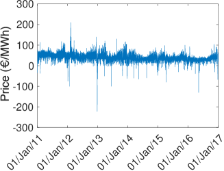
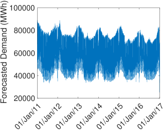
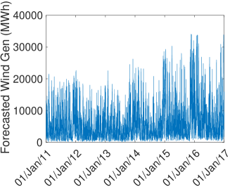
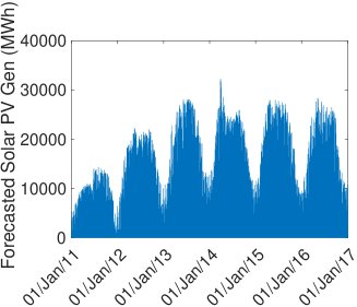
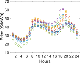
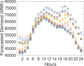
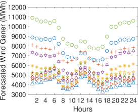
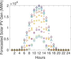
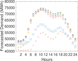
To summarize, we use daily fossil fuel prices (, gas, and coal, denoted by , and , respectively, and kept constant over the 24 hours) and hourly data (with daily frequency) for electricity prices, forecasted demand (denoted by ), wind (denoted by ), and solar PV generation (denoted by ) from 01 January 2011 to 31 December 2016 for Germany and Denmark and from 13 June 2014 to 13 June 2017 for Italy and Spain. We use the first four years as an estimation sample for Germany and Denmark, and the first two for Italy and Spain, whereas we use the last two/one years as the forecast evaluation period. The historical dynamics of these series observed in Germany are reported in Figure 1. Prices show clearly the new stylized fact of “downside” spikes together with mean-reversion, whereas forecasted demand and solar generation exhibit more clear yearly seasonal patterns, with an increasing trend for solar power generation according to the new capacity additions through years. Similarly, forecasted wind shows its dependence on weather conditions albeit with an increasing trend,999Given that trends can be observed in the studied series, we have tested that its inclusion does not improve substantially the forecasting performance. corresponding again to investments in new capacity. To highlight calendar seasonality, monthly profiles for electricity prices, forecasted demand, and wind and solar generation are depicted in Figure 2. Furthermore, to emphasize the weekly seasonality, Figure 3 depicts the intra-daily dynamics across days of the weeks for demand and prices; obviously, wind and solar are not presented, as they are weather-dependent. Similar figures for the other countries are reported in Section S.1 of the Supplementary Material.
 |
 |
 |
 |
 |
 |
 |
 |
 |
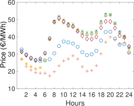 |
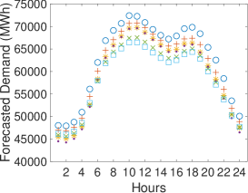
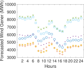
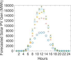
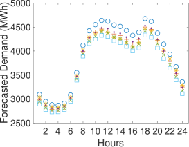
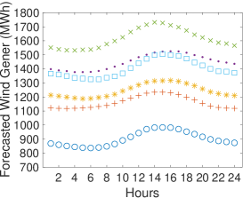
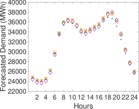
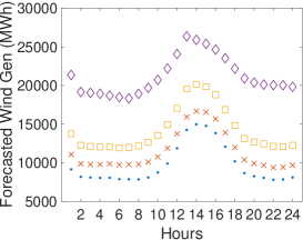
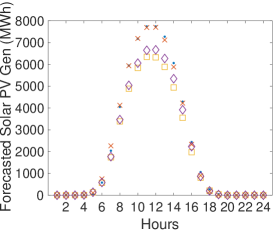
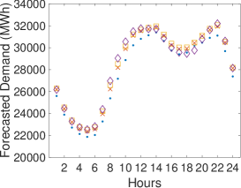
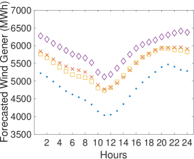
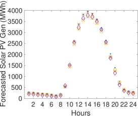
Finally, the intra-daily profiles for the yearly average values of forecasted demand and RES-E are represented in Figure 4 to identify scenarios of high/low demand and/or RES-E expected to affect prices and, consequently, forecasts. We can observe that the ramp-up hours (during which the demand for electricity is expected to grow substantially) as well as the ramp-down hours (when demand is expected to decrease sharply) change across markets according to day- and night-time and geographical locations. However, they confirm higher demand levels in the peak period (roughly between 8 a.m. and 8 p.m. for all markets). The intra-daily profiles for wind show different dynamics: we can again identify scenarios for high wind generation during peak hours in Denmark and Italy, whereas the opposite occurs in Germany and Spain. Obviously, the intra-daily profiles for solar PV generation are, instead, common for all markets, where available. Therefore, we can expect a stronger combined effect of high demand and wind in Denmark, and high demand, wind, and solar in Italy, but contrasting scenarios for demand, wind, and solar during the day in Germany and Spain: a low-high-low one (that is low demand and solar versus high wind) in the early and late hours versus a high-low-high one (that is high demand and solar versus low wind) for peak hours.
 |
 |
 |
 |
 |
|
 |
 |
 |
 |
 |
 |
4 Forecasting Models
We consider univariate and multivariate models for hourly prices with seasonality and with the introduction of exogenous variables relative to the forecasted demand and forecasted RES-E. Furthermore, we have included fossil fuels to account for marginal costs, hence reflecting the non-linearity of the supply curve. Specifically, coal, natural gas, and CO2 settlement prices have been included with a delay of one day, given that market operators do know their values determined at the market closure of the day before (that is on day ) when they run their models early in the morning on day to submit the 24-hour price forecasts by 11 a.m. (of the same day) for trades occurring on the following day, .
Therefore, we have specified the following models to compare the forecasting performances when demand, RES-E, and fossil fuels are taken into account. There is unanimous consensus that including demand forecasts or RES-E forecasts (if the market penetration is not negligible) leads to more accurate forecasts. However, it is still an open question as to which RES forecast is more informative in which market and also whether their inclusion can reduce the importance of fossil fuels; hence, models with only a subset of exogenous variables have also been considered. All together results, first, in inspecting simple models with only dummy variables for seasonality; second, in adding regressors accounting for both demand and supply curves (that is dummies plus forecasted demand and lagged fossil fuels); third, in considering if the forecasting ability of demand and RES reduces the need of including fuels; and finally, in verifying if only forecasted wind and/or solar generation is/are efficient in providing good price forecasts. We follow common practice in the literature and restrict lags to and , which correspond to the previous day, two days before, and one week before delivery time, recalling, first, similar conditions that may have characterized the market over the same hours and similar days (like congestions and blackouts) and, second, the demand level during the days of the week. Knittel and Roberts, (2005), Weron and Misiorek, (2008) and Raviv et al., (2015) show that these specifications provide accurate forecasts because they capture seasonal patterns in electricity prices. In addition, this formulation reduces the risk of overparameterization. Hence, hourly prices with a reduced 7-lag structure are considered, and, with an abuse of notation in the remainder of the paper, is used in all our univariate and multivariate models to denote the number of included lags, instead of the maximum lag.
4.1 Multivariate Models
We consider and compare the performances of two different multivariate model specifications with and without exogenous variables, used as benchmarks for the corresponding multivariate models. These are the VAR model, the VAR model with exogenous variables (VARX) estimating by using Least Square (OLS), see equations (2.3.2) and (2.3.4) in Kilian and Lutkepohl, (2017), and their Bayesian formulations (BVAR and BVARX, respectively) with a normal-Wishart prior, see Section S.2 of the Supplementary Material.
4.1.1 Vector Autoregressive Model – VAR
Let denote the vector of hourly electricity prices, with . Moreover, we denote with the dummy vector with representing the twelve months of the year and representing Saturdays and Sundays, hence . The VAR model of order is formulated as follows:
| (1) |
where is the matrix containing the autoregressive coefficients as well as the coefficients for all dummy variables, and is the matrix made by the lagged electricity prices and the dummy variables. The vector of errors is assumed to be serially uncorrelated and normally distributed with zero mean and a full covariance matrix .
4.1.2 Vector Autoregressive Model with Exogenous Variables – VARX
The VARX includes the forecasted demand, as well as the forecasted wind and solar power generation, when available, and fossil fuel prices for coal, gas, and . The exogenous demand and RES variables are represented by the following vectors of dimensions , , and , respectively. On the other hand, fuel prices do not change over the 24 hours and are determined on the previous day, . Thus, , and are the representations for , gas, and coal at previous time, respectively. From (1), we re-define the matrix as and, consequently, the matrix of coefficients of size . The matrix now comprises the vector of lagged hourly electricity prices, the vectors of dummy variables, and the exogenous variables. From eq. (1), as the observations vary with time , the VAR and VARX models of order can be rewritten in a compact way
| (2) |
where is an matrix, and is the matrix of explanatory variables containing all the exogenous variables.101010We have also performed the forecasting exercises including the lags (1,2, and 7) for exogenous variables, but the results were unchanged although computationally intensive and time-demanding. For these reasons, and having proper forecasts, we prefer to adopt the former models without lagged exogenous variables. The error matrix is normally distributed and serially uncorrelated with covariance matrix .
4.1.3 Bayesian Vector Autoregressive Models – BVARs
Our multivariate models with or without exogenous variables have been additionally estimated using the Bayesian methodology. From eq. (2), a BVAR or BVARX has the following stacked form
| (3) |
where , are vectorized matrices, with being a -dimensional identity matrix. This stacked form representation allows us to define and study the prior and posterior distribution of the matrix of coefficients and covariance matrix leading to a closed form distribution. In particular, we define prior information on the matrix of coefficients and on the covariance matrix using a conjugate normal-Wishart prior.111111We have performed the analysis using both a standard Minnesota and the normal-Wishart priors, and the results are similar. Therefore, due to lack of space, we have reported only the results for the latter. Details on the prior information and posterior distribution are reported in Section S.2 of the Supplementary Material.
4.2 Univariate Models
For all previous models, we formulate 24 (parsimonious) univariate AR specifications with the same assumptions on the lag order of the VAR specifications, whereas the errors are assumed to be normally distributed with zero mean and variance for the hours . The autoregressive model with only dummy variables is used as benchmark in the forecasting comparisons and can be written as follows
On the other hand, the univariate ARX or BARX can be written as
where and represent (forecasted) demand and renewable energy variables, whereas and are the fossil fuel prices previously described. Even in the univariate case, we use both the frequentist and the Bayesian estimation procedures.
To support the multivariate formulation, we run univariate models with dummies, lags of , and fundamentals lagged same-hour prices, adding also the first lag of all other remaining hours, that is
Then, from the resulting 24 residual series of each model, , the variance-covariance matrix has been computed. Uncorrelated residuals make the multivariate VAR specification unnecessary; however, we find evidence of large correlations across all studied markets121212These results have been omitted for lack of space, but they are available on request.. Therefore, a VAR with full covariance matrix seems more appropriate to estimate this covariance structure and it should result in improved density forecast accuracy.
4.3 Forecast Assessment
We assess the goodness of our forecasts using different point and density metrics. Considering the accuracy of point forecasts, we use the root mean square errors (RMSEs) for each of the hourly prices, as well as the RMSEs on the daily average and on an average restricted only to central hours, as specified below. The RMSE for hourly prices is computed as
| (4) |
where is the number of observations, is the length of the rolling window and are the individual hourly price forecasts. In addition, we analyse the average RMSEs on all the 24 hours () and on the hours from 8 a.m. to 8 p.m. (peak hours, ), computed as follows:
| (5) | ||||
| (6) |
To evaluate density forecasts, we use the average continuous ranked probability score (CRPS).131313We computed also that the log predictive score and results were similar; hence, they have not been reported.
As indicated in Gneiting and Raftery, (2007) and Gneiting and Ranjan, (2011), some researchers view the continuous ranked probability score as having advantages over the log score. In particular, the CRPS does a better job of rewarding values from the predictive density that are close to - but not equal to - the outcome, and it is less sensitive to outlier outcomes. The CRPS, defined such that a lower number is a better score, is given by
where denotes the cumulative distribution function associated with the predictive density , denotes an indicator function taking the value if and otherwise, and and are independent random draws from the posterior predictive density. In the same way we can construct the average CRPS over the 24 hours and over peak hours on day .
More specifically, we report the RMSEs and average CRPS for all the univariate and multivariate models and for every third hour.141414Tables with all hours are available in Section S.4, S.5, S.6 and S.7 of the Supplementary Material.
In addition, we apply Diebold and Mariano, (1995) t-tests for equality of the average loss (with loss defined as squared error or CRPS) to compare predictions of alternative models to the benchmark for a given horizon 151515In our application for testing density forecasts, we use equal weights without adopting a weighting scheme, as in Amisano and Giacomini, (2007).. The differences in accuracy that are statistically different from zero are denoted with one, two, or three asterisks, corresponding to significance levels of 10%, 5%, and 1%, respectively. The underlying p-values are based on t-statistics computed with a serial correlation-robust variance, using the pre-whitened quadratic spectral estimator of Andrews and Monahan, (1992). Our use of the Diebold-Mariano test, with forecasts from models that are, in many cases, nested, is a deliberate choice, as in Clark and Ravazzolo, (2015), and, as noted by Clark and West, (2007) and Clark and McCracken, (2012), this test is conservative and might result in under-rejection of the null hypothesis of equal predictability. We report p-values based on one-sided tests, taking the AR (VAR) as the null and the other current models as the alternative.
Finally, we have also applied the Model Confidence Set procedure of Hansen et al., (2011) across models for a fixed horizon to jointly compare their predictive power without disentangling between univariate and multivariate models. The R package MCS detailed in Bernardi and Catania, (2016) has been used, and the differences have been tested separately for each hour and model, repeating the full process across all countries. Results are discussed in the following section.
5 Results
Our results are based on a one-step-ahead forecasting process with a rolling window approach of 4 years for Germany and Denmark and of 2 years for Italy and Spain. Let us recall that we have two estimation samples 01/01/2011–31/12/2014 for Germany and Denmark, and 13/06/2014–13/06/2016 for Italy and Spain. And then we have two forecast evaluation periods: 01/01/2015–31/12/2016 for the former two markets (for a total of 731 observations), and 14/06/2016–13/06/2017 for the latter two countries (hence, only 365 observations).
Before evaluating the out-of-sample results, our in-sample evidence provides statistically significant coefficients for the RES variables in all markets; hence, confirming the empirical findings in previous literature on univariate models augmented with RES variables and extending similar conclusions also to multivariate models. In particular, coefficients of wind and solar are negative in Germany, Italy, and Spain. Also in Denmark, wind has a negative coefficient.161616Detailed in-sample results are available under request. These results confirm that renewable energy sources are significantly connected to and reduce electricity prices. Therefore, we continue our analysis by investigating whether these relationships can result in forecast gains.
To this end, our results show the performance of our different univariate and multivariate models from the simplest ones (with only dummy variables, the benchmarks) to more complex ones containing gas, coal, , and forecasts for demand, wind, and solar. Alternative formulations referred to subsets of drivers are described in Table S.1 of the Supplementary Material, and results are summarized in Tables 1 and 2 across all markets at every third hours; whereas extensive comparisons are shown in Tables S.2–S.9 of the Supplementary Material.
Recalling the main objectives of this analysis, we have shown clearly the superiority of multivariate models when the full structure of 24 hours is considered. Multivariate VAR models outperform simple AR models when only seasonality is included. This holds true systematically across all countries, and according to both point and density metrics. For instance, in Germany, the average RMSE moves from 8.259 €/MWh in the univariate case to 6.839 €/MWh in the multivariate case. In Spain, it goes from 6.299 €/MWh to 5.110 €/MWh. The case is similar for the CRPSs for which we observe substantial reductions of almost 18% (from 4.427 to 3.643) in Germany, 13% (from 4.901 to 4.273) in Denmark, 5% (from 3.658 to 3.469) in Italy, and 20% (from 3.517 to 2.831) in Spain, for average values computed over the 24 hours. The AR models are included in the model confidence set in only 10 cases over 64 horizons in the two Tables 1 and 2 for both metrics and mainly for the Italian market. VAR models have a much higher frequency of inclusion. Hence, this supports our expectations of more efficient forecasts obtained considering the interrelationships among the whole 24 hours, as suggested by Stock and Watson, (2002) and anticipated by Raviv et al., (2015).
Moreover, considering the most important fact, that is the forecasting improvements to the inclusion of RES and/or a subset of drivers, our results show that the Bayesian multivariate models with forecasted RES-E and fuels exhibit substantial improvements generally in all markets. Average reductions in loss function are similar for both metrics and from 10% to 20% in Germany and Spain and from 1% to 5% for Denmark and Italy. Forecast gains increase in the peak hours, as shown in columns Avg8-20. When focusing on each individual hour, BVARXs statistically outperform VAR models and they are included in the model confidence set in most of the cases, and almost always for late morning, afternoon and evening hours. VARX models also perform accurately, but give some economically smaller gain than do BVARX models.
Going into details and exploring the forecasting ability of several models with different combinations of variables to inspect their individual contribution, we first find evidence of forecasting improvements when demand and all RES are included. Moreover, the BVAR model with only forecasted wind (besides forecasted demand and fuels) leads to better forecasts than are those obtained with the inclusion of only forecasted solar (besides forecasted demand and fuels), especially for point forecasts over hours 8-24 in Germany, Italy, and Spain (not performed in Denmark because there is no available solar power). Comparing the ability of the BVAR model with forecasted demand and RES with the one containing forecasted demand and fuels, the former is found to perform better. However, there are further gains when all these exogenous regressors are considered simultaneously.171717This may be due to the contribution of individual fuels. For instance, in an additional analysis within the frequentist approach, we have observed that models with selected fuels, forecasted demand and RES show slight improvements in the RMSEs: in Germany, the inclusion of both CO2 and coal improves the forecast accuracy over hours 8-24; in Denmark, the inclusion of only gas improves the forecast accuracy during hours 8-12, whereas coal improves over the remaining ones 13-24. In Italy, coal and gas together are important during rump-up and rump-down hours (9-10 & 18-19), whereas only gas is important during hours 11-17; this is consistent with Italy’s dependence on thermal generation (and so on traditional fuels), given the still marginal penetration of RES (compared to the other countries studied). In Spain, the inclusion of coal slightly and generally improves the forecast accuracy, which is, however, comparable with the model with all fuels at selected hours (12-15 & 23-24). In all these cases, adding the omitted fuels induces only very small reduction in the performances, hence supporting the conclusion of an overall importance of all fossil fuels when forecasting day-ahead electricity prices. These results are omitted for lack of space, but they are available on request.
6 Conclusions
This paper compares the forecasting performances of linear univariate and multivariate models with enlarged specifications. Our set of models includes autoregression and vector autoregression models with only dummy variables for seasonality, which are used as baseline for the corresponding formulations enlarged by including also fuels, demand and renewable energy sources, analysed from both the frequentist and the Bayesian perspective.
Our results indicate that models with demand, renewable energy, and fuels dominate those without fuels and renewable energy sources (RES), in terms of both point and density forecasting. In particular, the first important finding is that the multivariate models outperform the univariate ones, given that they allow for interrelationships among different hours of the day. Secondly, the Bayesian approach leads to further forecasting improvements. Thirdly, and for the first time since the increasing RES penetration, we show that the models with only forecasted wind perform better than those with solar power only. And, their simultaneous inclusion further improves the performance.
We also provide a strong empirical evidence of the influence of the renewable power generation during the day, and consistently with the country intra-daily profiles. In fact, during the first hours of the day, the models without forecasted RES-E are more accurate than those with them, and again with errors from multivariate models lower than those from univariate ones. Whilst, the increasing RES-E during the day leads to more accurate forecasts from augmented models. Furthermore, our results are consistent across all adopted scoring rules, such as the RMSE and the CRPS.
From an energy forecasting perspective these linear multivariate autoregressive models with RES, demand and fuels seem to have interesting and important advantages over the widely used univariate ones. It is worth emphasizing the increasing relevance of density forecasting since in these recent years market operators are exploring opportunistic bidding across market sessions, as emphasized by Bunn et al., (2018). Indeed, forecasting the day-ahead prices is important for market operators and traders to plan their strategy. For example, arbitrage opportunities can be explored by deciding on which market session to bid according to the forecasted day-ahead prices. For this reason, energy regulatory authorities are trying to formulate optimal pricing rules to avoid these market inefficiencies. Agents operating balancing responsible units are exposed to economic consequences from differentials between day-ahead and balancing prices, which are used to evaluate the actual unit imbalance according to the sign of the system imbalance. In simple words, if one unit is short-imbalanced when the market is long (or long-imbalanced when the market is short), it receives profits for relieving the system (which are computed on the basis of price differentials). Otherwise, if unit and system have signs agreement, the unit receives penalties because it aggravates the system imbalance.
All these considerations clearly show the extreme relevance of both point and density forecasting for these day-ahead electricity prices and our results highlight that the Bayesian multivariate models with considered drivers improve them substantially.
Acknowledgements
Authors thank the co-editor, seminar and conference participants at Ca’ Foscari University of Venice, the EU Joint Research Centre in Ispra, the University of Warwick, the ‘26th Annual Symposium of the Society for Nonlinear Dynamics and Econometrics’ in Tokyo, the ‘15th Conference on Computational Management Science’ in Trondheim, the ‘12th Annual RCEA Bayesian Econometric Workshop’ in Rimini, and the ‘8th Energy Finance Christmas Workshops’ in Bozen for useful comments and suggestions. This research used the SCSCF multiprocessor cluster system at Ca’ Foscari University of Venice. Europe Energy S.p.A. is acknowledged for funding this research project. In addition, Angelica Gianfreda wishes to acknowledge the RTDcall2017 support for the project on Forecasting and Monitoring electricity Prices, volumes and market Mechanisms, funded by the Free University of Bozen-Bolzano. Luca Rossini acknowledges the financial support from the EU Horizon 2020 under the Marie Sklodowska-Curie scheme (grant agreement No 796902).
References
- Amisano and Giacomini, (2007) Amisano, G. and Giacomini, R. (2007). Comparing density forecasts via weighted likelihood ratio tests. Journal of Business & Economic Statistics, 25(2):177–190.
- Andrews and Monahan, (1992) Andrews, D. and Monahan, J. (1992). An improved heteroskedasticity and autocorrelation consistent covariance matrix estimator. Econometrica, 60(4):953–966.
- Bernardi and Catania, (2016) Bernardi, M. and Catania, L. (2016). Portfolio Optimisation Under Flexible Dynamic Dependence Modelling. ArXiv e-prints.
- Bunn et al., (2018) Bunn, D. W., Gianfreda, A., and Kermer, S. (2018). A trading-based evaluation of density forecasts in a real-time electricity market. Energies, 11(10):2658–2670.
- Chen and Bunn, (2014) Chen, D. and Bunn, D. (2014). The forecasting performance of a finite mixture regime-switching model for daily electricity prices. Journal of Forecasting, 33(5):364–375.
- Clark and McCracken, (2012) Clark, T. E. and McCracken, M. W. (2012). Reality checks and comparisons of nested predictive models. Journal of Business & Economic Statistics, 30(1):53–66.
- Clark and Ravazzolo, (2015) Clark, T. E. and Ravazzolo, F. (2015). Macroeconomic forecasting performance under alternative specifications of time-varying volatility. Journal of Applied Econometrics, 30(4):551–575.
- Clark and West, (2007) Clark, T. E. and West, K. D. (2007). Approximately normal tests for equal predictive accuracy in nested models. Journal of Econometrics, 138(1):291–311.
- Conejo et al., (2005) Conejo, Contreras, Espínola, and Plazas (2005). Forecasting electricity prices for a day-ahead poolbased electric energy market. International Journal of Forecasting, 21(3):435–462.
- Diebold and Mariano, (1995) Diebold, F. and Mariano, R. (1995). Comparing predictive accuracy. Journal of Business and Economic Statistics, 13(3):253–263.
- García-Martos et al., (2007) García-Martos, C., Rodríguez, J., and Sánchez, M. J. (2007). Mixed models for short-run forecasting of electricity prices: Application for the spanish market. IEEE Transactions on Power Systems, 22(2):544–552.
- Gelabert et al., (2011) Gelabert, L., Labandeira, X., and Linares, P. (2011). An ex-post analysis of the effect of renewables and cogeneration on spanish electricity prices. Energy Economics, 33, Supplement 1:S59 – S65. Supplemental Issue: Fourth Atlantic Workshop in Energy and Environmental Economics.
- Gianfreda and Bunn, (2018) Gianfreda, A. and Bunn, D. (2018). A stochastic latent moment model for electricity price formation. Operations Research, 66:1189–1456.
- Gianfreda and Grossi, (2012) Gianfreda, A. and Grossi, L. (2012). Forecasting Italian electricity zonal prices with exogenous variables. Energy Economics, 34(6):2228–2239.
- Gianfreda et al., (2016) Gianfreda, A., Parisio, L., and Pelagatti, M. (2016). Revisiting long-run relations in power markets with high RES penetration. Energy Policy, 94:432 – 445.
- Gianfreda et al., (2018) Gianfreda, A., Parisio, L., and Pelagatti, M. (2018). A review of balancing costs in Italy before and after RES introduction. Renewable and Sustainable Energy Reviews, 91:549 – 563.
- Gianfreda et al., (2019) Gianfreda, A., Parisio, L., and Pelagatti, M. (2019). The RES-induced switching effect across fossil fuels: An analysis of day-ahead and balancing prices. The Energy Journal, 40.
- Gneiting and Raftery, (2007) Gneiting, T. and Raftery, A. (2007). Strictly proper scoring rules, prediction and estimation. Journal of American Statistical Association, 102(477):359–378.
- Gneiting and Ranjan, (2011) Gneiting, T. and Ranjan, R. (2011). Comparing density forecasts using threshold and quantile weighted proper scoring rules. Journal of Business and Economic Statistics, 29(3):411–422.
- Hansen et al., (2011) Hansen, P. R., Lunde, A., and Nason, J. M. (2011). The Model Confidence Set. Econometrica, 79:453–497.
- Hirth and Ziegenhagen, (2015) Hirth, L. and Ziegenhagen, I. (2015). Balancing power and variable renewables: Three links. Renewable and Sustainable Energy Reviews, 50:1035 – 1051.
- Huurman et al., (2012) Huurman, C., Ravazzolo, F., and Zhou, C. (2012). The power of weather. Computational Statistics and Data Analysis, 56(11):3793–3807.
- Jónsson et al., (2010) Jónsson, T., Pinson, P., and Madsen, H. (2010). On the market impact of wind energy forecasts. Energy Economics, 32(2):313 – 320.
- Jónsson et al., (2014) Jónsson, T., Pinson, P., Madsen, H., and Nielsen, H. A. (2014). Predictive densities for day-ahead electricity prices using time-adaptive quantile regression. Energies, 7(9):5523–5547.
- Karakatsani and Bunn, (2008) Karakatsani, N. V. and Bunn, D. W. (2008). Forecasting electricity prices: The impact of fundamentals and time-varying coefficients. International Journal of Forecasting, 24(4):764 – 785.
- Ketterer, (2014) Ketterer, J. C. (2014). The impact of wind power generation on the electricity price in germany. Energy Economics, 44:270 – 280.
- Kilian and Lutkepohl, (2017) Kilian, L. and Lutkepohl, H. (2017). Structural Vector Autoregressive Analysis. Cambridge University Press, Themes in Modern Econometrics.
- Knittel and Roberts, (2005) Knittel, C. and Roberts, M. (2005). An empirical examination of restructured electricity prices. Energy Economics, 27(5):791–817.
- Koopman et al., (2007) Koopman, S. J., Ooms, M., and Carnero, M. A. (2007). Periodic seasonal reg-arfima-garch models for daily electricity spot prices. Journal of the American Statistical Association, 102(477):16–27.
- Lisi and Edoli, (2018) Lisi, F. and Edoli, E. (2018). Analyzing and forecasting zonal imbalance signs in the italian electricity market. The Energy Journal, 39(5).
- Maciejowska and Nowotarski, (2016) Maciejowska, K. and Nowotarski, J. (2016). A hybrid model for gefcom2014 probabilistic electricity price forecasting. International Journal of Forecasting, 32(3):1051 – 1056.
- Maciejowska and Weron, (2015) Maciejowska, K. and Weron, R. (2015). Forecasting of daily electricity prices with factor models: utilizing intra-day and inter-zone relationships. Computational Statistics, 30(3):805–819.
- Maciejowska and Weron, (2016) Maciejowska, K. and Weron, R. (2016). Short- and mid-term forecasting of baseload electricity prices in the u.k.: The impact of intra-day price relationships and market fundamentals. IEEE Transactions on Power Systems, 31(2):994–1005.
- Martinez-Anido et al., (2016) Martinez-Anido, C. B., Brinkman, G., and Hodge, B.-M. (2016). The impact of wind power on electricity prices. Renewable Energy, 94(Supplement C):474 – 487.
- Mauritzen, (2013) Mauritzen, J. (2013). Dead battery? wind power, the spot market, and hydropower interaction in the nordic electricity market. Energy Journal, 34(1):103–123.
- Misiorek et al., (2006) Misiorek, A., Trueck, S., and Weron, R. (2006). Point and interval forecasting of spot electricity prices: linear vs. non-linear time series models. Studies in Nonlinear Dynamics & Econometrics, 10(2).
- Nowotarski and Weron, (2018) Nowotarski, J. and Weron, R. (2018). Recent advances in electricity price forecasting: A review of probabilistic forecasting. Renewable and Sustainable Energy Reviews, 81(Part 1):1548 – 1568.
- Panagiotelis and Smith, (2008) Panagiotelis, A. and Smith, M. (2008). Bayesian density forecasting of intraday electricity prices using multivariate skew t distributions. International Journal of Forecasting, 24(4):710 – 727.
- Paraschiv et al., (2014) Paraschiv, F., Erni, D., and Pietsch, R. (2014). The impact of renewable energies on EEX day-ahead electricity prices. Energy Policy, 73:196 – 210.
- Pircalabu et al., (2017) Pircalabu, A., Hvolby, T., Jung, J., and Høg, E. (2017). Joint price and volumetric risk in wind power trading: A copula approach. Energy Economics, 62:139 – 154.
- Poplavskaya and de Vries, (2019) Poplavskaya, K. and de Vries, L. (2019). Distributed energy resources and the organized balancing market: A symbiosis yet? case of three european balancing markets. Energy Policy, 126:264 – 276.
- Raviv et al., (2015) Raviv, E., Bouwman, K. E., and van Dijk, D. (2015). Forecasting day-ahead electricity prices: Utilizing hourly prices. Energy Economics, 50:227 – 239.
- REN21, (2017) REN21 (2017). Renewables 2017 - global status report, (paris: Ren21 secretariat). ISBN 978-3-9818107-6-9.
- Rintamäki et al., (2017) Rintamäki, T., Siddiqui, A. S., and Salo, A. (2017). Does renewable energy generation decrease the volatility of electricity prices? an analysis of Denmark and Germany. Energy Economics, 62:270 – 282.
- Stock and Watson, (2002) Stock and Watson (2002). Forecasting using principal components from a large number of predictors. Journal of American Statistical Association, 97(460):1167–1179.
- Uniejewski et al., (2016) Uniejewski, B., Nowotarski, J., and Weron, R. (2016). Automated variable selection and shrinkage for day-ahead electricity price forecasting. Energies, 9(621).
- Weron, (2014) Weron, R. (2014). Electricity price forecasting: A review of the state-of-the-art with a look into the future. International Journal of Forecasting, 30(4):1030 – 1081.
- Weron and Misiorek, (2008) Weron, R. and Misiorek, A. (2008). Forecasting spot electricity prices: A comparison of parametric and semiparametric time series models. International Journal of Forecasting, 24(4):744–763.
- Woo et al., (2011) Woo, C., Horowitz, I., Moore, J., and Pacheco, A. (2011). The impact of wind generation on the electricity spot-market price level and variance: The Texas experience. Energy Policy, 39(7):3939 – 3944. Special Section: Renewable energy policy and development.
- Ziel and Weron, (2018) Ziel, F. and Weron, R. (2018). Day-ahead electricity price forecasting with high-dimensional structures: Univariate vs. multivariate modeling frameworks. Energy Economics, 70:396 – 420.
Hour 1 4 7 10 13 16 19 22 Avg Germany AR 7.240 7.387 8.027 8.905 9.214 9.669 8.692 6.277 8.259 9.333 ARX (FD+RES+Fuels) 5.336∗∗∗ 5.939∗∗ 6.430∗∗∗ 6.928∗∗∗ 6.662∗∗∗ 7.068∗∗∗ 6.867∗∗∗ 4.871∗∗∗ 6.326 7.065 BAR 7.226∗∗ 7.387 8.011∗∗ 8.887∗∗∗ 9.214 9.659∗∗∗ 8.666∗∗∗ 6.258∗∗∗ 8.251 9.314 BARX (FD+RES+Fuels) 5.329∗∗∗ 5.932∗∗ 6.430∗∗∗ 6.768∗∗∗ 6.597∗∗∗ 7.068∗∗∗ 6.728∗∗∗ 4.821∗∗∗ 6.260 6.972 VAR 4.278 4.944 6.271 6.905 7.934 8.350 8.290 6.164 6.839 7.993 VARX (FD+RES+Fuels) 4.492 5.404 6.396 6.083∗∗∗ 6.315∗∗∗ 7.039∗∗∗ 6.715∗∗∗ 4.654∗∗∗ 5.964 6.698 BVAR 4.282 4.939 6.271 6.912 7.934 8.342 8.290 6.158 6.839 7.993 BVARX (FD+RES+Fuels) 4.445 5.414 6.415 6.035∗∗∗ 6.276∗∗∗ 6.964∗∗∗ 6.591∗∗∗ 4.629∗∗∗ 5.923 6.642 Denmark AR 5.850 6.566 6.857 13.162 8.226 8.029 10.300 6.012 8.468 10.465 ARX (FD+RES+Fuels) 5.376 6.211 6.082∗∗∗ 9.661∗∗∗ 6.893∗∗∗ 6.544∗∗∗ 8.240∗∗∗ 5.345∗ 6.969 8.121 BAR 5.838∗∗ 6.553∗∗∗ 6.843∗∗∗ 13.096∗∗∗ 8.210∗∗∗ 8.021∗∗∗ 10.279∗∗∗ 6.000∗∗∗ 8.451 10.444 BARX (FD+RES+Fuels) 5.382 6.211 6.089∗∗∗ 9.635∗∗∗ 6.885∗∗∗ 6.552∗∗∗ 8.219∗∗∗ 5.339∗ 6.961 8.110 VAR 3.413 4.131 5.159 10.913 7.607 7.466 10.441 5.897 7.197 9.328 VARX (FD+RES+Fuels) 4.386 5.684 5.690 10.553 6.778∗∗ 6.421∗∗∗ 8.750∗∗∗ 5.213∗∗∗ 6.974 8.460 BVAR 3.413 4.135 5.164 10.913 7.599∗∗∗ 7.451∗∗∗ 10.431∗∗ 5.891∗∗ 7.190 9.319 BVARX (FD+RES+Fuels) 4.386 5.680 5.690 10.553 6.755∗∗∗ 6.421∗∗∗ 8.760∗∗∗ 5.201∗∗∗ 6.974 8.451 Italy AR 4.560 4.405 5.162 9.107 6.389 8.122 9.835 7.104 6.838 8.331 ARX (FD+RES+Fuels) 4.410 4.185 4.966 8.561 5.776∗∗∗ 7.513∗∗ 9.638 6.862 6.469 7.806 BAR 4.551 4.401 5.157 9.098∗∗ 6.389 8.122∗ 9.835 7.111 6.831 8.331 BARX (FD+RES+Fuels) 4.432 4.238 4.961∗ 8.524∗∗ 5.756∗∗∗ 7.488∗∗∗ 9.560∗ 6.870 6.455 7.764 VAR 3.884 4.105 4.753 8.569 6.144 7.650 9.582 6.893 6.507 7.901 VARX (FD+RES+Fuels) 4.094 4.228 4.881 8.098 5.511∗∗∗ 7.107∗∗ 9.668 6.996 6.357 7.530 BVAR 3.880 4.101 4.753 8.569 6.150 7.650 9.572∗∗ 6.893∗ 6.507 7.901 BVARX (FD+RES+Fuels) 4.051 4.142 4.853 8.106 5.523∗∗∗ 7.061∗∗ 9.649 6.934 6.325 7.506 Spain AR 7.036 6.741 7.066 6.421 6.140 6.873 5.574 4.628 6.299 6.389 ARX (FD+RES+Fuels) 0.809∗∗∗ 0.779∗∗∗ 0.776∗∗∗ 0.804∗∗∗ 0.813∗∗∗ 0.796∗∗∗ 0.883∗∗ 1.020 0.825 0.814 BAR 0.999∗ 0.998∗∗∗ 0.997∗∗∗ 0.994∗∗∗ 0.997∗∗∗ 0.997∗∗∗ 0.994∗∗∗ 0.996∗∗∗ 0.996 0.996 BARX (FD+RES+Fuels) 0.818∗∗∗ 0.798∗∗∗ 0.805∗∗∗ 0.844∗∗∗ 0.838∗∗∗ 0.815∗∗∗ 0.903∗∗ 1.040 0.847 0.839 VAR 3.943 4.638 5.227 4.761 5.018 5.908 5.363 4.823 5.110 5.317 VARX (FD+RES+Fuels) 1.001 0.940 0.843∗∗∗ 0.855∗∗∗ 0.825∗∗∗ 0.752∗∗∗ 0.791∗∗∗ 0.858∗∗ 0.834 0.801 BVAR 1.000 1.000 1.000 0.998 0.999 0.997∗∗ 0.993∗∗∗ 0.994∗∗∗ 0.998 0.997 BVARX (FD+RES+Fuels) 1.010 0.952∗ 0.856∗∗∗ 0.860∗∗∗ 0.829∗∗∗ 0.757∗∗∗ 0.797∗∗∗ 0.860∗∗ 0.841 0.806 • Notes: 1 Forecast errors are calculated using rolling window estimation. ‘Avg’ and ‘Avg8-20’ stand for RMSEs computed as in (5) and (6). 2 Please refer to Section 4 for details on model formulations. The ‘X’ indicates models with exogenous variables, while ‘B’ Bayesian conjugate Normal-Wishart priors. 3 ∗∗∗, ∗∗ and ∗ indicate RMSE ratios are significantly different from 1 at , and , according to Diebold-Mariano test. 4 Gray cells indicate those models that belong to the Superior Set of Models delivered by the Model Confidence Set procedure at confidence level .
Hour 1 4 7 10 13 16 19 22 Avg Germany AR 3.770 4.062 4.467 4.942 4.962 4.970 4.792 3.423 4.427 4.964 ARX (FD+RES+Fuels) 2.926∗∗∗ 3.420∗∗∗ 3.672∗∗∗ 3.781∗∗∗ 3.563∗∗∗ 3.593∗∗∗ 3.786∗∗∗ 2.663∗∗∗ 3.422 3.733 BAR 3.770 4.062 4.458∗ 4.927∗∗∗ 4.957∗ 4.960∗∗ 4.768∗∗∗ 3.409∗∗∗ 4.418 4.954 BARX (FD+RES+Fuels) 2.926∗∗∗ 3.420∗∗∗ 3.672∗∗∗ 3.702∗∗∗ 3.528∗∗∗ 3.598∗∗∗ 3.719∗∗∗ 2.646∗∗∗ 3.391 3.688 VAR 2.261 2.901 3.443 3.772 4.185 4.208 4.525 3.347 3.643 4.173 VARX (FD+RES+Fuels) 2.390 3.040 3.443 3.316∗∗∗ 3.294∗∗∗ 3.509∗∗∗ 3.692∗∗∗ 2.570∗∗∗ 3.169 3.497 BVAR 2.254∗∗ 2.886∗∗∗ 3.426∗∗∗ 3.764∗∗ 4.177∗∗ 4.191∗∗∗ 4.507∗∗∗ 3.334∗∗∗ 3.632 4.160 BVARX (FD+RES+Fuels) 2.358 3.037 3.426 3.282∗∗∗ 3.260∗∗∗ 3.472∗∗∗ 3.615∗∗∗ 2.554∗∗∗ 3.137 3.451 Denmark AR 3.236 3.690 3.896 8.844 4.400 4.156 5.379 3.188 4.901 6.199 ARX (FD+RES+Fuels) 2.997∗∗∗ 3.446∗∗∗ 3.471∗∗∗ 7.517∗∗∗ 3.670∗∗∗ 3.387∗∗∗ 4.255∗∗∗ 2.866∗∗∗ 4.210 5.151 BAR 3.230∗∗ 3.683∗∗ 3.892 8.817∗∗∗ 4.387∗∗∗ 4.148∗∗ 5.368∗∗ 3.182∗∗ 4.891 6.187 BARX (FD+RES+Fuels) 2.997∗∗∗ 3.443∗∗∗ 3.475∗∗∗ 7.509∗∗∗ 3.665∗∗∗ 3.387∗∗∗ 4.249∗∗∗ 2.866∗∗∗ 4.210 5.151 VAR 2.019 2.644 3.035 7.829 3.925 3.761 5.329 3.100 4.273 5.606 VARX (FD+RES+Fuels) 2.314 3.093 3.199 7.727∗ 3.556∗∗∗ 3.295∗∗∗ 4.487∗∗∗ 2.737∗∗∗ 4.119 5.219 BVAR 2.007∗∗∗ 2.631∗∗∗ 3.020∗∗∗ 7.790∗∗∗ 3.901∗∗∗ 3.731∗∗∗ 5.308∗∗∗ 3.088∗∗∗ 4.247 5.572 BVARX (FD+RES+Fuels) 2.300 3.067 3.178 7.743∗ 3.532∗∗∗ 3.268∗∗∗ 4.460∗∗∗ 2.725∗∗∗ 4.106 5.208 Italy AR 2.547 2.460 2.851 4.772 3.494 4.390 5.037 3.616 3.657 4.413 ARX (FD+RES+Fuels) 2.476 2.362∗ 2.731∗∗ 4.514∗∗ 3.141∗∗∗ 4.100∗∗∗ 4.992 3.522∗∗ 3.481 4.157 BAR 2.539∗∗ 2.455 2.854 4.767 3.491 4.386 5.032 3.609∗∗ 3.653 4.409 BARX (FD+RES+Fuels) 2.488 2.386 2.720∗∗ 4.457∗∗∗ 3.113∗∗∗ 4.039∗∗∗ 4.881∗∗ 3.511∗∗ 3.449 4.095 VAR 2.147 2.265 2.588 4.509 3.342 4.095 4.954 3.569 3.469 4.177 VARX (FD+RES+Fuels) 2.291 2.378 2.694 4.356 3.008∗∗∗ 3.812∗∗ 5.177 3.744 3.455 4.043 BVAR 2.145 2.263 2.580∗ 4.482∗∗∗ 3.329∗∗ 4.075∗∗∗ 4.924∗∗∗ 3.551∗∗∗ 3.452 4.156 BVARX (FD+RES+Fuels) 2.259 2.310 2.653 4.338 2.991∗∗∗ 3.763∗∗∗ 5.157 3.708 3.417 4.014 Spain AR 3.914 3.757 3.948 3.555 3.402 3.844 3.139 2.669 3.517 3.556 ARX (FD+RES+Fuels) 3.112∗∗∗ 2.915∗∗∗ 3.064∗∗∗ 2.901∗∗∗ 2.786∗∗∗ 3.037∗∗∗ 2.734∗∗∗ 2.613 2.891 2.895 BAR 3.910 3.746 3.952 3.541 3.388 3.832 3.117 2.658 3.503 3.538 BARX (FD+RES+Fuels) 3.151∗∗∗ 2.987∗∗∗ 3.190∗∗∗ 3.040∗∗∗ 2.858∗∗∗ 3.106∗∗∗ 2.787∗∗∗ 2.666 2.961 2.973 VAR 2.128 2.536 2.897 2.644 2.743 3.267 3.019 2.745 2.831 2.945 VARX (FD+RES+Fuels) 2.145 2.381∗ 2.422∗∗∗ 2.239∗∗∗ 2.271∗∗∗ 2.447∗∗∗ 2.364∗∗∗ 2.306∗∗∗ 2.350 2.350 BVAR 2.122 2.526 2.885 2.631 2.724 3.244 2.989 2.720 2.814 2.924 BVARX (FD+RES+Fuels) 2.164 2.414 2.471∗∗∗ 2.250∗∗∗ 2.263∗∗∗ 2.440∗∗∗ 2.373∗∗∗ 2.306∗∗∗ 2.361 2.353 • Notes: 1 Forecast errors are calculated using rolling window estimation. ‘Avg’ and ‘Avg8-20’ stand for average CRPS for average values. 2 Please refer to Section 4 for details on model formulations. The ‘X’ indicates models with exogenous variables, while ‘B’ Bayesian conjugate Normal-Wishart priors. 3 ∗∗∗, ∗∗ and ∗ indicate average score ratios are significantly different from 1 at , and , according to Diebold-Mariano test. 4 Gray cells indicate those models that belong to the Superior Set of Models delivered by the Model Confidence Set procedure at confidence level .