Fundamental Properties of Co-Moving Stars observed by $Gaia$

Abstract

We have estimated fundamental parameters for a sample of co-moving stars observed by $Gaia$ and identified by Oh et al. (2017b). We matched the $Gaia$ observations to the 2MASS and WISE catalogs and fit MIST isochrones to the data, deriving estimates of the mass, radius, $[Fe/H]$, age, distance and extinction to 9,754 stars in the original sample of 10,606 stars. We verify these estimates by comparing our new results to previous analyses of nearby stars, examining fiducial cluster properties, and estimating the power-law slope of the local present-day mass function. A comparison to previous studies suggests that our mass estimates are robust, while metallicity and age estimates are increasingly uncertain. We use our calculated masses to examine the properties of binaries in the sample, and show that separation of the pairs dominates the observed binding energies and expected lifetimes.

binaries: general — stars: fundamental parameters — catalogs

1 Introduction

Stars with similar space motions, also known as co-moving stars, are unique testbeds for stellar and Galactic investigations. They encompass a variety of separations, from $\sim 1$ AU, up to the widest separations observed ($\sim$ 10 pc; Raghavan et al., 2010; Oh et al., 2017b). They can be used as probes of star formation (i.e., Elliott et al., 2016), planetary system survival (Kaib et al., 2013; Kaib & Raymond, 2014) and Galactic dynamics (Jiang & Tremaine, 2010). Widely separated pairs are of particular utility, as they are sensitive to the mass spectrum of large perturbers in the Milky Way, including giant molecular clouds and black holes (Bahcall et al., 1985; Weinberg et al., 1986, 1987). They are also sensitive to the overall mass distribution since they are easily disrupted by Galactic tidal forces (e.g., Opik, 1976; Hurley et al., 2002; Jiang & Tremaine, 2010). When widely separated pairs of stars are found, the individual stellar members serve to form a cluster of stars with $N=2$, making them benchmarks for calibrating age and metallicity relations (i.e., Dhital et al., 2012; Rojas-Ayala et al., 2012).

Modern surveys have identified thousands of co-moving binaries within a few kpc of the Sun (Dhital et al., 2010, 2015; Oelkers et al., 2017; Oh et al., 2017b; Andrews et al., 2017). These survey studies have identified a new population of stars with separations of $<1$ to 10 pc ($10^{2}$–$10^{6}$ AU) easily some of the widest pairs known. These pairs were identified using parallaxes and proper motions from $Gaia$. For the comparison of true 3D velocity vectors, radial velocities (RVs) are required (Andrews et al., 2017; Price-Whelan et al., 2017). At the largest separations, the false positive rate grows, reaching $\sim 60\%$, making RVs critical for identifying true companions (Price-Whelan et al., 2017). With the approach of $Gaia$ data release 2, which includes the RVs of millions of bright stars ($G<12$), many more co-moving stars should be discovered.

Despite these advances, the fundamental properties of the widest pairs are not well constrained. First, binary interactions, moving groups and other phase-space structure can produce stars with similar motions that may not have begun their existence as bound companions, breaking the common assumption of co-eval and co-metallicity. Next, pair-identifying algorithms can fracture larger ensembles of co-moving stars, shredding moving groups into isolated pairs. Algorithms designed to work in observable space (i.e., R.A., Dec., proper motion) are more prone to this issue than those working in $XYZUVW$ space. Finally, since the identification is mostly derived from the astrometric properties of the stars, the fundamental properties of the stars themselves, masses, ages and metallicities, have not been characterized.

In this paper, we explore the fundamental properties (mass, radius, [Fe/H], age, and extinction) of thousands of widely separated pairs. We derive these properties from an ensemble of survey observations, along with isochronal fits to each star. In Section 2, we describe the $Gaia$ observations and the catalog of Oh et al. (2017b), which we use for this analysis. The Oh et al. (2017b) catalog was recently reorganized and re-analyzed by Faherty et al. (2018), which we adopt for this analysis. We supplement the $Gaia$ observations with archival photometry from ground and space-based telescopes. In Section 3, we provide estimates of fundamental parameters for all stars in the catalog, including mass, age, and metallicity. Our estimates are verified by comparisons to prior studies and known fiducial clusters, including the Pleiades and Hyades. In Section 4, we explore our results, including an analysis of the mass properties of the binary systems. Finally, our conclusions are presented in Section 5.

2 Observations

Below we describe the observations used in our analysis. Our catalog incorporates $Gaia$ photometry and astrometry, as well as photometry obtained during the Two-Micron All-Sky Survey (2MASS; Skrutskie et al., 2006) and by the Wide-Field Infrared Sky Explorer satellite (WISE; Wright et al., 2010).

2.1 $Gaia$ Observations

The $Gaia$ satellite (Gaia Collaboration et al., 2016a) was launched in December 2013 and will map the entire sky over 5 years, producing the largest and most precise astrometric catalog yet. The final catalog is expected to contain the sky positions, proper motions and distances to $\sim$ 1 billion unique stars, with a typical parallax, $\varpi$, uncertainty of $\sigma_{\varpi}\sim$ 20 $\mu$as for a Sun-like star with $G$ = 15.

The $Gaia$ satellite images the sky using two telescopes separated by a basic angle of 106.5^∘ focusing light onto a focal plane of 106 CCDs (Gaia Collaboration et al., 2016b). The first data release from the $Gaia$ team included proper motions and parallaxes for about 2.0 million nearby bright stars observed by Tycho-2 and Hipparcos. The Tycho-$Gaia$ Astrometric Solution catalog (TGAS; ESA, 1997; Høg et al., 2000; van Leeuwen, 2007; Michalik et al., 2015; Lindegren et al., 2016) contains mostly bright stars, with 90% of the catalog having $G<12.05$. The median uncertainty in parallax and position is 0.32 mas, with proper motion uncertainties of 1.32 mas yr^-1 (Lindegren et al., 2016). Bovy (2017) has shown that the TGAS catalog is mostly complete to a distance of $\sim$ 200 pc for main-sequence spectral types A through K.

The Oh et al. (2017b) sample of co-moving stars, later examined and re-organized by Faherty et al. (2018), was drawn from the TGAS sample. We summarize the basic sample construction here, and refer the reader to Oh et al. (2017b) and Faherty et al. (2018) for details. The Oh et al. (2017b) sample first applied a global signal-to-noise cut on the parallaxes in the TGAS catalog, retaining 619,618 stars with $[S/N]_{\varpi}$ > 8. Next, they searched for stars with similar space motions and 3D separations $<10$ pc. They identified 271,232 pairs of stars meeting these criteria, then applied a statistical selection, based on a fully marginalized likelihood, to identify the most likely pairs. The final Oh et al. (2017b) catalog contained 10,606 individual stars organized into 4,236 unique groups with over 319 of those groups containing 3 or more stars (triples or higher order). Faherty et al. (2018) re-analyzed the groups identified by Oh et al. (2017b) using the BANYAN $\Sigma$ code (Gagné et al., 2018, 2017a, 2017b) as well as a literature search and found many of the hierarchical groups were parts of known clusters (i.e., the Pleiades, $\alpha$ Per, and the Hyades clusters) and nearby moving groups and associations (e.g., Lower Centaurus Crux, Upper Centaurus Lupus). However known stellar members of associations were also broken up across several unique Oh et al. (2017b) groups. For example, Faherty et al. (2018) recorded Hyades members found within 8 groups identified by Oh et al. (2017b) and members of the Lower Centaurus Crux association were found in 26 different groups. We refer the reader to Faherty et al. (2018) for a complete discussion of the re-organized sample.

2.2 Cross Matching with 2MASS and WISE

In order to compare observed data on our pairs to model isochrones, we supplemented $Gaia$ photometry with near-infrared (NIR) data from 2MASS and mid infrared data (MIR) from the WISE mission.

The 2MASS project employed two identical 1.3m telescopes in the Northern and Southern hemispheres to systematically map the night sky in the $J$ (1.1 $\mu$m), $H$ (1.8 $\mu$m) and $K_{s}$ (2.2 $\mu$m) bands. The northern telescope was located at the Whipple Observatory on Mount Hopkins in Arizona, USA, while the southern telescope was found at the Cerro-Tololo Inter-American Observatory at Cerro-Tololo, Chile. Over the course of 3 years, the 2MASS project recorded 24.5 TB of raw images, resulting in an all-sky catalog of over 470 million objects, which are mostly point sources. The point-source catalog (PSC) is complete to $J<15.8,H<15.1,K_{s}<14.3$, when confusion is unimportant. Typical uncertainties on the photometric observations are $\sim 1-2\%$, while the astrometric uncertainties for the most of the PSC is 0.07-0.08 arcseconds.

The Wide-Field Infrared Survey Explorer (WISE Wright et al., 2010) satellite imaged the entire sky in four infrared bands, centered on 3.4, 4.6, 12, and 22 $\mu$m, and named $W1$, $W2$, $W3$ and $W4$ respectively. The mission surveyed the sky during 2010, covering most of the sky at least twice during that time. The telescope recorded images of over 560 million objects during its primary mission, and was restarted to search for near–Earth asteroids as NEOWISE (Mainzer et al., 2011). Combining both programs resulted in the AllWISE catalog (Cutri & et al., 2013), which contains 747,634,026 objects and is 95% complete to $W1<17.1$, $W2<15.7$, $W3<11.5$ and $W4<7.7$. Typical astrometric precision is 0.15 arcseconds.

Using the Tool for OPerations on Catalogues And Tables (TOPCAT Taylor, 2005), we implemented a 1$\arcsec$ radial search between the positions in Gaia and those in the ALLWISE catalog and recovered $W1W2W3W4$ photometry. ALLWISE also automatically identifies matches with the 2MASS point source catalog using a 2$\arcsec$ radius therefore we also recovered $JHK_{s}$ photometry with one TOPCAT query. After implementing our match, 598 Gaia positions lacked a WISE measurement, and an additional 13 lacked 2MASS photometry. Therefore the full sample we used in the isochrone analysis below contained 9,995 unique stars from the Oh et al. (2017b) catalog.

3 Analysis - Fundamental Parameter Estimation

We used the isochrone python module (Morton, 2015) to estimate the fundamental parameters (mass, age, radius, $[Fe/H]$, distance, and extinction) of each star in our sample. The package uses the Mesa Isochrones and Stellar Track library (MIST; Dotter, 2016; Choi et al., 2016; Paxton et al., 2011, 2013, 2015) and computes the posterior probability of fundamental parameters given the data. The MIST isochrones span $[Fe/H]$ from -4.00 to -2.00 in 0.50 dex steps and from -2.00 to +0.50 in 0.25 dex steps, and $\log{\frac{\rm Age}{\rm Gyr}}$ from 5.0 to 10.3 in 0.05 dex steps. The isochrones are available in many standard bandpass sets, including $Gaia$, 2MASS and WISE.

We computed posterior probabilities on mass, age, radius, $[Fe/H]$, distance, and extinction for the sample conditioned on the measurements of $\varpi,G,J,H,K$, and $W1$ and their uncertainties. These posteriors were calculated using the trilinear interpolation schemes within isochrones and assumed priors described in Morton (2015), including a distance prior from the parallax reported by $Gaia$ and a $[Fe/H]$ prior from metallicity estimates (Bovy, 2016) of nearby stars by Casagrande et al. (2011). The extinction prior for each star was bounded at its maximum value with an extinction estimate calculated from the reddening reported in the Schlegel et al. (1998), using the re-calibrated values (Schlafly & Finkbeiner, 2011) and the Fitzpatrick (1999) reddening law. Next, the posterior distributions were sampled using the MCMC ensemble sampler emcee (Foreman-Mackey et al., 2013). We initialized 500 walkers with a random initialization bounded by values described by Morton (2015) and allowed them to explore the posterior probabilities for 100 iterations. The sampler was then re-initialized as at the location with the highest likelihood, with a small Gaussian perturbation in all dimensions. The walkers then ran for 700 steps, with a burn-in of 200 steps, and the last 500 steps were recorded. The fundamental parameters listed were obtained by taking the median posterior sample, along with the 15% and 85% percentile samples. We compared the posterior samples of each parameter to their priors and observed differences, indicating the supplemental photometry aided in constraining the model parameters. An example of our posterior samples are shown in Figure 1. For 241 stars, the sampler was unable to converge upon a solution. Therefore we report fundamental parameters for 9,754 of our input sample. All resultant fundamental parameters (mass, age, radius, $[Fe/H]$, distance, and extinction) are listed in Table 1 and summarized in Figure 2.

Table 1: Fundamental Parameters

TGAS Source ID	R.A. (deg)	Dec. (deg)	Mass ($M_{\odot}$)	Radius ($R_{\odot}$)	[Fe/H] (dex)	log(age (yr))	Distance (pc)	$A_{v}$ (mag)
49809491645958528	59.4573	18.5622	$0.81^{+0.06}_{-0.06}$	$0.83^{+0.03}_{-0.04}$	$-0.09^{+0.15}_{-0.16}$	$9.97^{+0.34}_{-0.23}$	$130.8^{+5.0}_{-5.4}$	$0.10^{+0.07}_{-0.11}$
66939848447027584	57.0704	25.2149	$1.22^{+0.05}_{-0.05}$	$1.53^{+0.09}_{-0.10}$	$0.07^{+0.09}_{-0.11}$	$9.58^{+0.10}_{-0.08}$	$130.4^{+6.1}_{-6.9}$	$0.07^{+0.05}_{-0.05}$
50905051903831680	58.0034	19.5967	$1.07^{+0.05}_{-0.04}$	$1.10^{+0.04}_{-0.05}$	$0.12^{+0.15}_{-0.11}$	$9.56^{+0.24}_{-0.18}$	$147.4^{+5.8}_{-6.4}$	$0.11^{+0.07}_{-0.10}$
51452746133437696	59.5072	20.6766	$1.21^{+0.05}_{-0.06}$	$1.30^{+0.08}_{-0.09}$	$-0.07^{+0.11}_{-0.13}$	$9.30^{+0.29}_{-0.19}$	$131.5^{+8.2}_{-8.7}$	$0.13^{+0.07}_{-0.04}$
51619115986889472	58.3703	20.9072	$0.79^{+0.03}_{-0.04}$	$0.81^{+0.03}_{-0.03}$	$0.11^{+0.11}_{-0.12}$	$10.13^{+0.26}_{-0.13}$	$132.2^{+4.2}_{-4.4}$	$0.09^{+0.06}_{-0.07}$
51674916201705344	58.8832	21.0793	$0.84^{+0.06}_{-0.06}$	$0.87^{+0.04}_{-0.04}$	$-0.03^{+0.14}_{-0.13}$	$9.97^{+0.35}_{-0.22}$	$123.4^{+4.6}_{-4.8}$	$0.08^{+0.06}_{-0.07}$
51694741770737152	59.5902	21.2575	$0.83^{+0.05}_{-0.05}$	$0.85^{+0.03}_{-0.04}$	$-0.03^{+0.14}_{-0.16}$	$9.98^{+0.31}_{-0.20}$	$138.0^{+5.3}_{-5.6}$	$0.08^{+0.06}_{-0.05}$
51742467447748224	58.6161	21.3895	$0.92^{+0.05}_{-0.05}$	$0.92^{+0.03}_{-0.04}$	$-0.00^{+0.11}_{-0.09}$	$9.75^{+0.42}_{-0.26}$	$134.6^{+4.7}_{-5.2}$	$0.09^{+0.06}_{-0.06}$
51861420861864448	62.2309	20.3858	$1.19^{+0.07}_{-0.07}$	$1.30^{+0.07}_{-0.07}$	$-0.04^{+0.14}_{-0.13}$	$9.38^{+0.29}_{-0.20}$	$126.1^{+6.0}_{-6.4}$	$0.13^{+0.09}_{-0.11}$
53783848223326976	60.9341	22.9441	$1.16^{+0.09}_{-0.07}$	$1.39^{+0.08}_{-0.09}$	$0.09^{+0.16}_{-0.14}$	$9.64^{+0.18}_{-0.15}$	$137.3^{+6.3}_{-7.1}$	$0.15^{+0.09}_{-0.06}$
61519668439604992	52.8682	21.8217	$1.29^{+0.01}_{-0.03}$	$1.44^{+0.05}_{-0.04}$	$-0.11^{+0.09}_{-0.06}$	$9.27^{+0.14}_{-0.07}$	$125.2^{+3.2}_{-4.8}$	$0.11^{+0.05}_{-0.05}$
62413983709539584	49.4574	22.8320	$1.70^{+0.07}_{-0.10}$	$2.17^{+0.12}_{-0.13}$	$-0.03^{+0.13}_{-0.17}$	$9.06^{+0.11}_{-0.08}$	$129.3^{+4.9}_{-5.3}$	$0.10^{+0.07}_{-0.09}$
63052044051306112	56.2570	19.5592	$1.21^{+0.08}_{-0.07}$	$1.39^{+0.08}_{-0.09}$	$-0.01^{+0.13}_{-0.15}$	$9.47^{+0.27}_{-0.17}$	$135.4^{+6.6}_{-7.7}$	$0.13^{+0.09}_{-0.08}$
63144712265008512	55.6245	20.1498	$1.49^{+0.09}_{-0.09}$	$1.58^{+0.10}_{-0.12}$	$-0.04^{+0.16}_{-0.14}$	$8.97^{+0.34}_{-0.20}$	$130.2^{+7.3}_{-8.8}$	$0.11^{+0.08}_{-0.11}$
63289916519862656	56.5807	20.8796	$0.82^{+0.06}_{-0.06}$	$0.84^{+0.04}_{-0.04}$	$-0.03^{+0.15}_{-0.16}$	$10.02^{+0.32}_{-0.20}$	$139.0^{+5.8}_{-6.3}$	$0.10^{+0.07}_{-0.06}$
63948214747182848	57.1640	21.9248	$1.38^{+0.04}_{-0.04}$	$1.70^{+0.10}_{-0.10}$	$-0.01^{+0.04}_{-0.05}$	$9.31^{+0.12}_{-0.08}$	$117.6^{+4.2}_{-4.6}$	$0.08^{+0.06}_{-0.04}$
64053561704835584	57.4796	22.2440	$2.38^{+0.06}_{-0.04}$	$3.12^{+0.25}_{-0.21}$	$-0.11^{+0.11}_{-0.14}$	$8.72^{+0.02}_{-0.02}$	$130.1^{+8.2}_{-7.5}$	$0.08^{+0.06}_{-0.07}$
64109911675780224	57.4092	22.5333	$2.10^{+0.06}_{-0.08}$	$1.91^{+0.12}_{-0.11}$	$0.00^{+0.01}_{-0.01}$	$8.48^{+0.20}_{-0.13}$	$128.3^{+4.8}_{-5.4}$	$0.07^{+0.03}_{-0.05}$
64114241002810496	57.2970	22.6093	$1.72^{+0.08}_{-0.08}$	$1.83^{+0.12}_{-0.13}$	$-0.01^{+0.11}_{-0.13}$	$8.86^{+0.22}_{-0.14}$	$130.6^{+6.2}_{-6.6}$	$0.10^{+0.07}_{-0.04}$
64172034082472448	57.5889	23.0962	$0.84^{+0.05}_{-0.06}$	$0.88^{+0.05}_{-0.07}$	$-0.00^{+0.14}_{-0.15}$	$10.04^{+0.37}_{-0.18}$	$138.6^{+9.2}_{-11.2}$	$0.10^{+0.07}_{-0.06}$
64313218247427456	54.8051	21.8431	$2.03^{+0.08}_{-0.08}$	$2.06^{+0.13}_{-0.13}$	$0.03^{+0.06}_{-0.09}$	$8.68^{+0.12}_{-0.10}$	$140.3^{+6.8}_{-6.8}$	$0.13^{+0.08}_{-0.11}$
64317994252099840	55.6001	21.4733	$1.11^{+0.04}_{-0.03}$	$1.16^{+0.04}_{-0.04}$	$-0.12^{+0.13}_{-0.11}$	$9.41^{+0.13}_{-0.14}$	$129.5^{+4.2}_{-3.8}$	$0.21^{+0.11}_{-0.11}$
64380632054140416	55.8798	22.1582	$1.05^{+0.05}_{-0.04}$	$1.07^{+0.04}_{-0.05}$	$0.14^{+0.13}_{-0.11}$	$9.63^{+0.24}_{-0.18}$	$134.6^{+4.6}_{-5.0}$	$0.10^{+0.06}_{-0.09}$
64449729487990912	55.6002	22.4210	$1.00^{+0.06}_{-0.06}$	$1.08^{+0.05}_{-0.05}$	$0.01^{+0.14}_{-0.14}$	$9.78^{+0.22}_{-0.16}$	$136.0^{+4.7}_{-5.1}$	$0.10^{+0.06}_{-0.07}$
64739244643463552	56.2456	22.0323	$1.23^{+0.05}_{-0.05}$	$1.36^{+0.07}_{-0.09}$	$-0.01^{+0.07}_{-0.05}$	$9.36^{+0.27}_{-0.16}$	$142.3^{+6.1}_{-7.5}$	$0.09^{+0.06}_{-0.07}$

Note. — This stubtable is a preview of the entire sample, which will be available as a machine readable table (and at https://github.com/jbochanski/gaia-wide-binaries/.

Figure 1: Upper Panel: A corner plot (Foreman-Mackey, 2016) of posterior samples derived from our analysis for one example star, TYC 9456-1172-1. The various panels are 2D projections along different axes of samples, along with histograms of the samples in $G,J,H,K$ and $W_{1}$. The observed values are overplotted as blue vertical lines. Lower Panel: A corner plot of the estimated fundamental parameters: mass, radius, [Fe/H], age, distance and $A_{V}$ for the star.

4 Discussion

In the following section, we discuss the results of our analysis. We begin with a validation of our analysis, by comparing our photometrically derived physical parameters to previous studies of the same stars. This is followed by an analysis of members (bona fide and suspected) of the nearby clusters. We also present color-magnitude diagrams with regard to fundamental parameters. Next, we examine the distributions of masses, compositions and ages recovered by our analysis. Finally, we discuss the mass ratio and binding energy distributions.

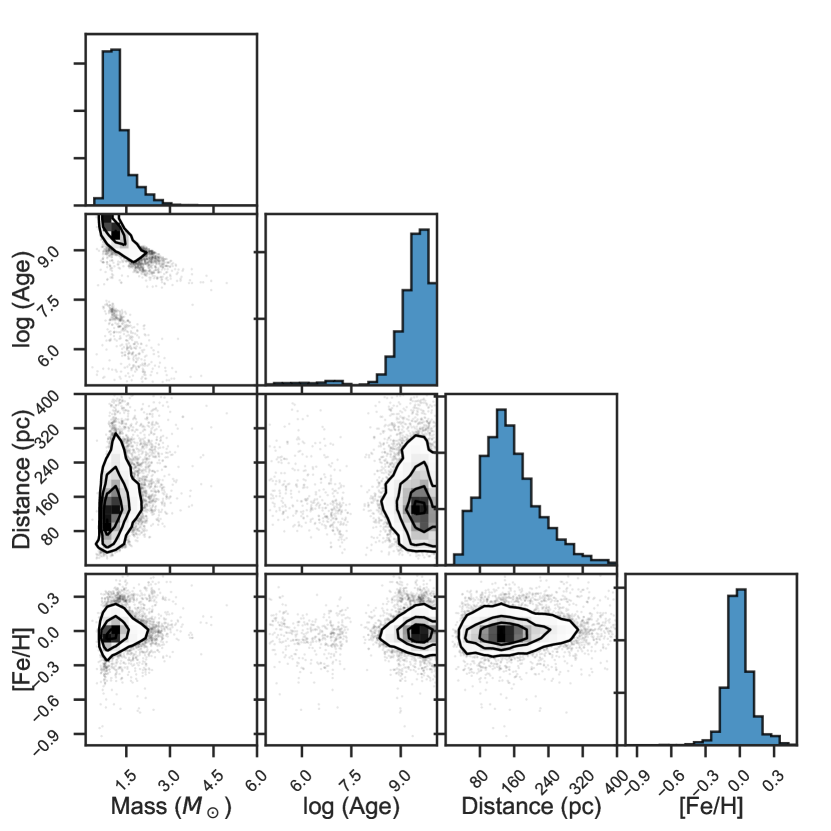
Figure 2: Corner plot of fundamental parameter for our entire sample. Most stars in our sample are solar metallicity, with estimated ages of $\sim 10^{9}$ years. There are no obvious correlations between mass and metallicity or age, which suggests that our mass estimates are robust.

4.1 Validation

4.1.1 Comparison to Geneva-Copenhagen Survey Members

We compare our photometrically derived fundamental parameters to the catalog of Casagrande et al. (2011), who re-analyzed the Geneva-Copenhagen Survey (GCS) of 16,682 FGK dwarfs with Stromgren photometry. Their work re-calibrated the temperature scale, and resulted in mass, age and metallicity estimates of the GCS sample. The catalogs were matched on Hipparcos catalog number. This yielded 672 matches between our sample and the Casagrande et al. (2011) catalog.

In Figure 3, we compare our fundamental parameter results to those from GCS for the stars in common between the two. Overall, the agreement in mass between the two catalogs is good. The same agreement is not seen with age and metallicity, indicating that these parameters may be less certain. We calculated the median and 15th and 85th percentiles of the differences between the two surveys (in the sense of GCS - this study). They are -0.03 ${}^{+0.08}_{-0.12}M_{\odot}$ for mass (using the Padova isochrones), 0.13 ${}^{+1.73}_{-2.03}\times 10^{9}$ yr for age, and -0.05 ${}^{+0.19}_{-0.19}$ dex for metallicity. In each case, the median difference between the two samples is consistent with zero.

Figure 3: We compare the masses (upper left) , metallicities (upper right) and ages (lower) derived in our analysis, compared to the same properties derived by Casagrande et al. (2011) for the 672 stars in common between GCS and our sample. We use the maximum likelihood values reported for the GCS stars using the Padova isochrones. Overall, the best agreement is seen in the mass estimates of the two analyses. We calculated the median and 15th and 85th percentiles (solid and dashed vertical lines) of the differences (GCS - this analysis). They are -0.03 ${}^{+0.08}_{-0.12}M_{\odot}$ for mass, 0.13 ${}^{+1.73}_{-2.03}\times 10^{9}$ yr for age, and -0.05 ${}^{+0.19}_{-0.19}$ dex for metallicity.

4.1.2 Comparing to Nearby Cluster and Moving Group Members

Next, we compared the derived fundamental properties to known clusters from Oh et al. (2017b) as identified in the reorganized catalog of Faherty et al. (2018). The groups with the largest number of members were the Pleiades (Cummings, 1921; Stauffer et al., 1989), $\alpha$ Per (Crawford & Barnes, 1974), and the Hyades open clusters (Perryman et al., 1998), and the Lower Centaurus Crux (LCC) group (Blaauw, 1946; de Zeeuw et al., 1999). In Figure 4 we show the derived fundamental parameters for the cluster members. The metallicity distributions for the four associations are quite similar, containing mostly solar metallicity stars, in agreement with most spectroscopic results. We over-plot literature estimates of the cluster metallicities as vertical lines. These are -0.01 for the Pleiades, 0.15 for the Hyades, 0.14 for $\alpha$ Per, and 0.0 for the LCC (Netopil et al., 2016; Cummings et al., 2017). The age distribution is shown in the upper right, along with literature estimates of the age of each group. The ages assumed are 130 Myr for the Pleiades (Barrado y Navascués et al., 2004), 85 Myr for $\alpha$ Per (Barrado y Navascués et al., 2004), 625 Myr for the Hyades (Perryman et al., 1998) and 17 Myr for the LCC moving group (Mamajek et al., 2002; Pecaut et al., 2012). Those values are over-plotted as vertical lines in the figure. Overall, the agreement between our derived values and literature estimates (often derived spectroscopically) is marginal, but the enhancement of Myr stars found in LCC indicates that some age discrimination is possible with isochrone fitting. In the lower left panel, we compare the derived distance estimates (based on the isochronal fitting with a prior derived from $Gaia$ observations) to literature estimates of the mean distance for each cluster. Due to the exquisite precision and accuracy of the $Gaia$ data, the agreement between our derived values and the literature values are good. The adopted average distances for the Pleiades (Mädler et al., 2016), $\alpha$ Per (van Leeuwen, 2009), Hyades (van Leeuwen, 2007) and LCC (de Zeeuw et al., 1999) are 135 pc, 172 pc, 47 and 118 pc, respectively. In lower right panel, we show the mass distributions of the four groups, which all share a similar slope. The Pleiades and Hyades demonstrate a larger number of observed low-mass stars, with $\alpha$ Per containing a larger fraction of high mass stars. However, since these are not complete surveys of the clusters, no strong statements can be made on intrinsic differences in the mass distributions. Overall, we find good agreement between our analysis and literature values for the metallicity and distance estimates, with less agreement between age estimates. This reflects the larger scatter seen in the age agreement in Section 4.1.1 and the challenges in estimating ages from photometry.

Figure 4: Histograms of fundamental parameters of identified members of the Pleiades (blue), $\alpha$ Per cluster(orange), Hyades (green) and Lower Centaurus-Crux moving group (red). Upper Left Panel: Most cluster members are found with metallicities close to solar. Literature estimates for mean metallicities are over-plotted as vertical lines Upper Right Panel: The ages of cluster members are shown, along with the mean ages of each cluster. The best age agreement is with the oldest cluster, the Hyades. Lower Left Panel: Distance estimates to cluster members, with average literature estimates over-plotted. Lower Right Panel: Mass estimates of cluster members. All four clusters show similar mass distributions.

In Figure 5, we plot the Gaia-2MASS color-magnitude diagram (CMD) of our total sample, along with members of the four clusters. The $G-K$ colors and $K$ magnitudes have not been corrected for extinction in any of the CMDS presented in this analysis. The Pleiades, $\alpha$ Per and Hyades members occupy similar areas of color-magnitude space, due to their similar ages and compositions. The LCC members demonstrate significant scatter. This is likely due to the the youth of the cluster, and the larger spread in distance, as seen in Figure 4. For each cluster, stars are found above the main sequence. For the older clusters, these are likely unresolved binaries, which are more common in wide binaries (Law et al., 2010), forming hierarchical multiple systems. Note that the stars identified as cluster members are not necessarily wide binaries.

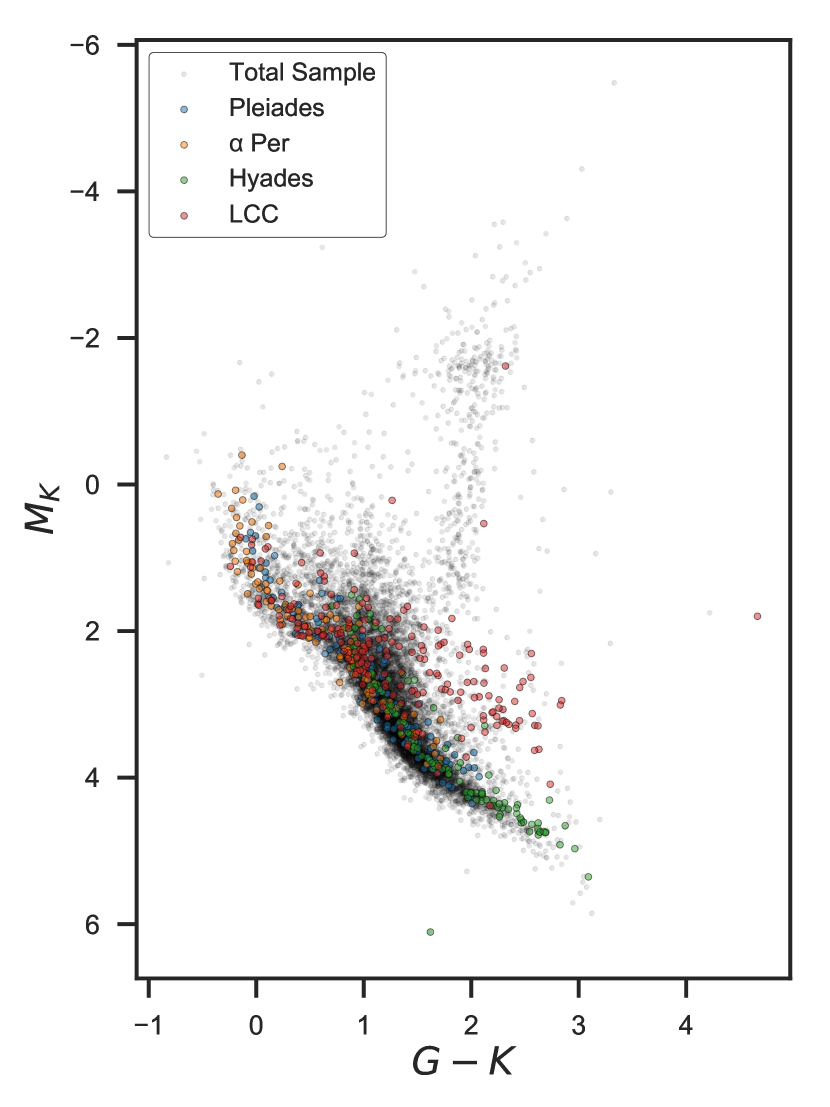
Figure 5: Color Magnitude Diagram ($M_{K}$ vs. $G-K$) of our sample, members of the Pleiades (blue), $\alpha$ Per (orange), Hyades (green), and Lower Centaurus Crux (red) overplotted. The Pleiades and Hyades contain the largest fraction of stars along the main sequence, while the LCC members show significant scatter. This scatter is likely due to the young age of the LCC.

4.1.3 Present–Day Mass Function

We further scrutinized our mass estimates by determining the present–day mass function (PDMF). The distribution of all masses can be found in Figure 2. For our PDMF measurement, we selected stars with masses $>1M_{\odot}$ within 200 pc, since TGAS is complete within 200 pc Bovy (2017) at these masses. The histogram of mass estimates for stars within 200 pc are shown in Figure 6. Bin sizes were chosen using Knuth’s rule (Knuth, 2006) as implemented in astroML (VanderPlas et al., 2014; Vanderplas et al., 2012; Ivezić et al., 2014). Solar-mass stars are the most common member of our sample, with low-mass stars (0.2-1.0 $M_{\odot}$) as the next most common constituent. The PDMF includes information on both the initial mass function (IMF, Bochanski et al., 2010) and the star formation rate. In Figure 7, we plot the number of stars per mass bin, in log-log scale, for stars with 1.0 $<M/M_{\odot}<$ 5.0 along with estimates of the posterior probability of a power-law fit. The slope of the power-law, commonly given as $\alpha$, where $\alpha=-2.35$ is the slope measured by Salpeter (1955), was $\alpha=-4.55\pm 0.05$, estimated by samples of the 16th, 50th, and 85th percentiles. While our sample is not complete, it is well matched to the estimates of the PDMF for $M>1M_{\odot}$ by Reid et al. (2002), $\alpha=-5.2\pm 0.4$ and the recently derived PDMF from Bovy (2017) $\alpha=-4.7$, which used a different set of isochrones to estimate masses of TGAS stars.

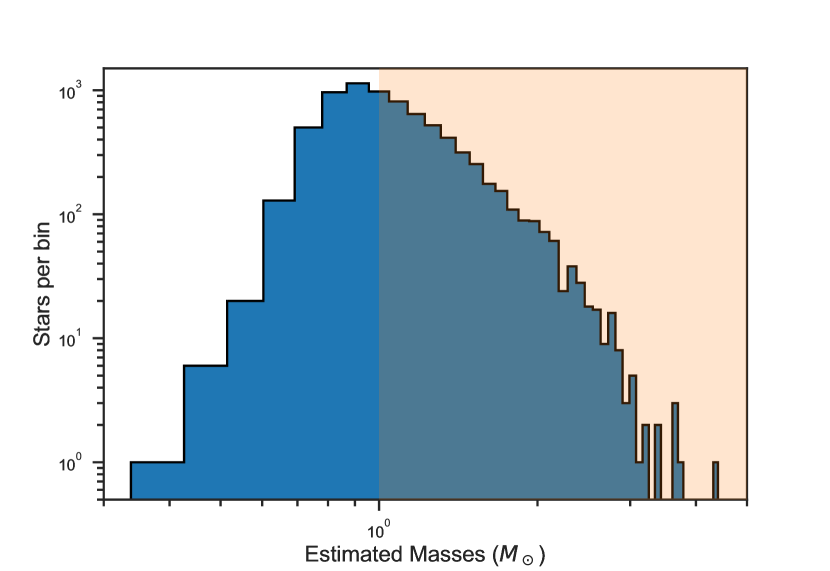
Figure 6: Histogram of mass estimates derived in our analysis for stars with distances less than 200 pc, where TGAS is mostly complete for spectral types A through K. We observe a peak at solar-mass stars, which should be complete in TGAS, and we note the falloff towards higher and lower masses. The low-mass falloff is due to incompleteness at low masses, while the decline towards higher masses is due to the PDMF. We selected stars with estimated masses $>1M_{\odot}$ for our PDMF analysis, which is shaded above.

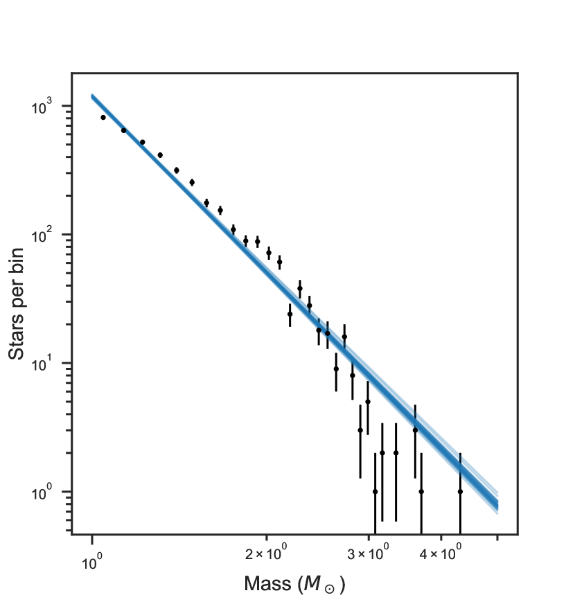
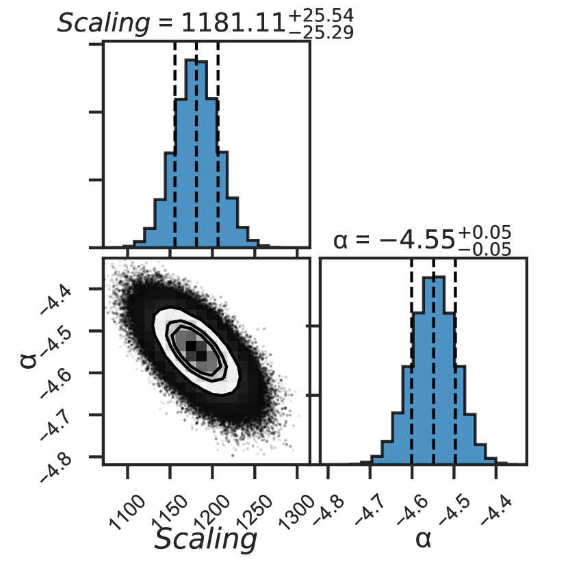
Figure 7: Left Panel: Stars per mass bin, in log-log scale, for stars with $M>1M_{\odot}$ stars. We sampled the posterior probabilities of a power-law fit to this distribution using emcee. Right Panel: The corner plot describing the fit to the mass distribution. We do not attempt measure the overall scaling of the mass function (in terms of stars per pc³), just the slope ($\alpha$) of the power-law fit. The slope agrees well with current estimates of the PDMF (Reid et al., 2002; Bovy, 2017).

4.2 Color–Magnitude Diagrams

In Figure 9, we plot color–magnitude diagrams of our sample in $M_{K}$ vs. $G-K$. The upper left panel highlights the $N=2$ pairs, with a line connecting each component, after Price-Whelan et al. (2017). The majority of the stars are found in pairs of main sequence stars, with a smaller subset containing a main sequence star with a red giant branch stars.

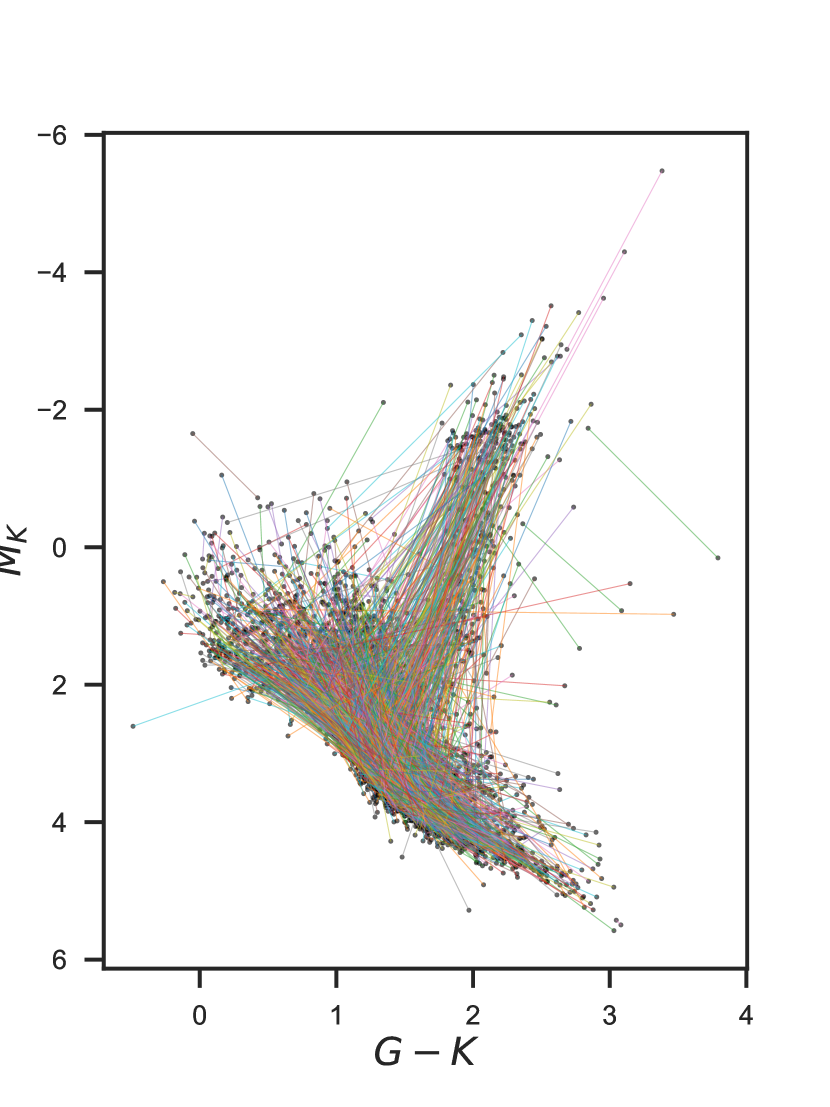
Figure 8: The color magnitude ($M_{K}$ vs. $G-K$) for pairs in our sample, after Price-Whelan et al. (2017). Each binary is connected by a colored line. Most of the sample is composed of main sequence $+$ main sequence pairs, but some main sequence $+$ red giant branch stars are observed.

Figure 9: Color–Magnitude Diagrams of our sample. In each window, $M_{K}$ vs. $G-K$ is shown. In panels a,b,c, and d each star is shaded by its log $g$, mass, age, and [Fe/H], respectively.

4.3 Binary Properties

We examined the properties of binaries in our sample. Co-moving binaries (with $N=2$) are usually assumed to be coeval members with similar compositions, but recent results have shown that pairs may not always have the same metallicity (i.e., Oh et al., 2017a). Below, we examine the differences in metallicity and age for pairs, and identify sets of "twin" stars in the sample. We also highlight the properties of the ten most widely-separated pairs. Finally, since our mass estimates are the most robust property measured, we examine the mass properties of the binaries, including their mass ratio and binding energy distributions, along with their expected dissipative lifetimes.

4.3.1 Metallicity and Age Distributions

As shown in Section 4.1, metallicity and age have significant uncertainties when estimated using photometry alone. In Figure 10 we examine the difference in $[Fe/H]$ and log age (yr) for the sample. In general the agreement in metallicity between members of binaries is good, with a broad peak centered on $\Delta_{[Fe/H]}=0$ and most stars agreeing within $\sim 0.2$ dex, on order with our external accuracy as determined in Section 4.1.1. Our large uncertainties with respect to age are evident in Figure 10, with some Myr stars being matched to Gyr counterparts. This is likely due to pairs containing members along the giant branch and main sequence. In Figure 9, many of the youngest stars can be found along the RGB, which suggests those ages are not trustworthy. These stars are being assigned ages appropriate for pre-main sequence (PMS) stars, which also affects their isochronal distance estimates, since RGB and PMS stars have much different luminosities. We confirmed this by comparing the parallactic and isochronal distances, and many RGB stars with erroneous young ages have large differences (> 50 pc) in their distance estimates.

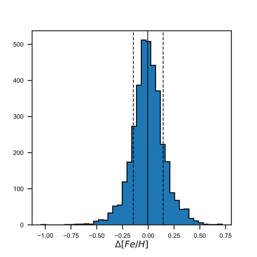
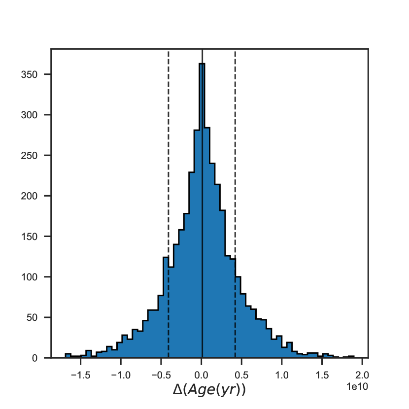
Figure 10: Left panel: Histogram of differences in [Fe/H] for binaries in our sample. The distribution is peaked at 0 with most stars agreeing within $\pm 0.2$ dex (standard deviation = 0.16 dex), which matches our external precision. Right Panel: Differences in ages between components. There is less agreement in the age estimates (standard deviation = 4 Gyr), which is likely due to the difficulties in estimating age from photometry alone. In both panels, the median (solid vertical line) and 15th and 85th percentiles (dashed vertical lines) are overplotted.

We also examined the differences in age and metallicity as a function of the separation of the individual stars. In Figure Figure 11, we show the differences as a function of separation, as well as the mean and standard deviation among 50 bins. There are no clear correlations with physical separation, which suggests that the pairs with large separations may be bona fide binaries. We also examined the distributions in age and metallicity differences in randomly associated pairs from our binary sample. For both age and metallicity, the standard deviation of differences was larger for the randomly associated stars as compared to our original sample.

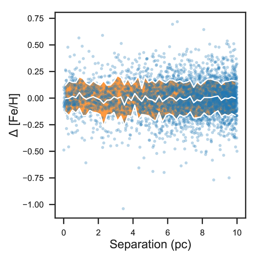
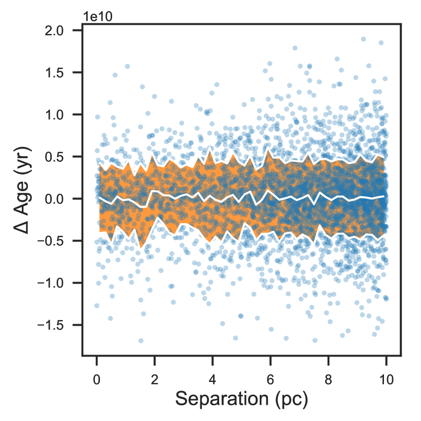
Figure 11: Left panel: Difference in estimated [Fe/H] vs. physical separation in pc. Right Panel: Difference in estimated age vs. physical separation in pc. Each filled circle represents a single binary system, and the means and standard deviations in 50 equally spaced bins are overplotted as the solid white line and filled orange area.

Despite the uncertainties in $[Fe/H]$ and age, we searched for binaries with identical members in terms of mass, age and composition. To select these twins, we enforced that the median estimates for both stars needed to match within 0.015 in mass, $[Fe/H]$ and log age. Three pairs of twins were identified, and summarized in Table 2.

Finally, we examined the ten pairs with the largest physical and projected separations. Their properties are summarized in Table 3 and Table 4. The pairs in Table 3 are presented in order of increasing separation, but they all have separations $\sim$ 10 pc, while the projected distances vary. As discussed in Oh et al. (2017b), the co-moving stars separated by the largest distances are most prone to false positives. Fundamental property estimates can test this, as false positives are unlikely to have the same metallicity and age. For the small sample in Table 3, that is not an issue, as many have metallicity estimates that agree within their uncertainties. Given the difficulty in photometrically estimating ages, coevality as determined by isochrone fitting cannot reliably rule out false positives. We also note that at least two pairs in Table 3 are main sequence stars paired with a red giant star.

Table 2: Stellar Twins

TGAS Source ID	R.A. (deg)	Dec. (deg)	Mass ($M_{\odot}$)	Radius ($R_{\odot}$)	[Fe/H] (dex)	log(age (yr))	Distance (pc)	$A_{v}$ (mag)	Sep. (pc)
3152809288677876992	106.1067	5.6167	$1.30^{+0.05}_{-0.05}$	$1.46^{+0.08}_{-0.09}$	$0.03^{+0.12}_{-0.08}$	$9.28^{+0.22}_{-0.14}$	$140.3^{+7.5}_{-7.6}$	$0.09^{+0.06}_{-0.09}$	8.6
3128405559378754560	104.8429	4.1459	$1.29^{+0.06}_{-0.07}$	$1.42^{+0.07}_{-0.08}$	$0.04^{+0.16}_{-0.11}$	$9.27^{+0.33}_{-0.19}$	$130.9^{+5.1}_{-5.2}$	$0.16^{+0.11}_{-0.16}$	8.6
5910699048908083840	262.1762	-62.4781	$0.82^{+0.05}_{-0.06}$	$0.86^{+0.03}_{-0.03}$	$0.02^{+0.14}_{-0.15}$	$10.06^{+0.35}_{-0.18}$	$132.6^{+4.1}_{-4.3}$	$0.04^{+0.03}_{-0.02}$	8.1
5816868066622162816	257.0792	-64.2002	$0.82^{+0.04}_{-0.05}$	$0.85^{+0.03}_{-0.03}$	$0.03^{+0.11}_{-0.13}$	$10.07^{+0.36}_{-0.18}$	$136.1^{+4.7}_{-5.2}$	$0.04^{+0.03}_{-0.04}$	8.1
5860448893617125120	182.6068	-66.5302	$1.04^{+0.07}_{-0.07}$	$1.10^{+0.06}_{-0.07}$	$-0.06^{+0.16}_{-0.15}$	$9.59^{+0.33}_{-0.24}$	$183.8^{+10.4}_{-11.9}$	$0.21^{+0.14}_{-0.19}$	9.5
5236357160153303808	175.1802	-66.5465	$1.05^{+0.06}_{-0.06}$	$1.12^{+0.06}_{-0.07}$	$-0.07^{+0.13}_{-0.16}$	$9.58^{+0.23}_{-0.19}$	$182.7^{+10.0}_{-11.2}$	$0.28^{+0.16}_{-0.16}$	9.5

Table 3: Pairs with largest physical separations

TGAS Source ID	R.A. (deg)	Dec. (deg)	Mass ($M_{\odot}$)	Radius ($R_{\odot}$)	[Fe/H] (dex)	log(age (yr))	Distance (pc)	$A_{v}$ (mag)	Sep. (pc)
1620697834607325056	222.4335	64.2362	$0.81^{+0.01}_{-0.02}$	$0.91^{+0.03}_{-0.03}$	$-0.10^{+0.06}_{-0.06}$	$10.12^{+0.02}_{-0.02}$	$216.5^{+12.5}_{-12.8}$	$0.01^{+0.00}_{-0.00}$	9.99
1668177735991697536	216.1852	64.6618	$1.13^{+0.03}_{-0.04}$	$1.25^{+0.04}_{-0.05}$	$-0.01^{+0.02}_{-0.00}$	$9.53^{+0.15}_{-0.12}$	$203.3^{+4.6}_{-9.7}$	$0.01^{+0.01}_{-0.00}$	9.99
5367018414717465728	159.5562	-44.4045	$0.96^{+0.09}_{-0.01}$	$0.88^{+0.03}_{-0.01}$	$0.13^{+0.18}_{-0.06}$	$9.36^{+0.06}_{-0.36}$	$232.1^{+8.7}_{-4.7}$	$0.04^{+0.00}_{-0.01}$	9.99
5366480031973428480	159.4605	-46.2679	$2.39^{+0.00}_{-0.00}$	$10.55^{+0.35}_{-0.56}$	$0.21^{+0.03}_{-0.02}$	$8.92^{+0.02}_{-0.02}$	$262.1^{+8.4}_{-12.6}$	$0.09^{+0.03}_{-0.05}$	9.99
2940892681712270464	93.1345	-21.4982	$1.71^{+0.10}_{-0.12}$	$1.65^{+0.13}_{-0.15}$	$-0.10^{+0.13}_{-0.16}$	$8.68^{+0.21}_{-0.18}$	$236.4^{+18.0}_{-22.5}$	$0.04^{+0.02}_{-0.02}$	9.99
2913756253703212416	93.0784	-22.4562	$0.83^{+0.04}_{-0.04}$	$0.88^{+0.05}_{-0.04}$	$0.07^{+0.16}_{-0.11}$	$10.09^{+0.19}_{-0.13}$	$244.3^{+14.5}_{-15.7}$	$0.02^{+0.02}_{-0.02}$	9.99
5321384833872077056	126.5134	-52.6093	$1.17^{+0.02}_{-0.01}$	$1.38^{+0.04}_{-0.04}$	$0.06^{+0.05}_{-0.06}$	$9.63^{+0.07}_{-0.05}$	$244.7^{+9.7}_{-9.0}$	$0.14^{+0.09}_{-0.14}$	9.99
5319637916053876224	125.1789	-54.4705	$1.07^{+0.05}_{-0.04}$	$1.07^{+0.06}_{-0.06}$	$-0.05^{+0.09}_{-0.11}$	$9.36^{+0.23}_{-0.19}$	$270.4^{+20.1}_{-20.0}$	$0.17^{+0.09}_{-0.08}$	9.99
6519199260800456832	340.1186	-46.4696	$1.00^{+0.04}_{-0.02}$	$0.92^{+0.03}_{-0.02}$	$0.04^{+0.14}_{-0.07}$	$9.14^{+0.30}_{-0.25}$	$118.4^{+4.3}_{-3.6}$	$0.00^{+0.00}_{-0.00}$	9.99
6517725709061049088	338.6571	-47.5968	$1.22^{+0.01}_{-0.01}$	$1.73^{+0.11}_{-0.17}$	$0.14^{+0.07}_{-0.05}$	$9.67^{+0.04}_{-0.02}$	$109.7^{+4.3}_{-7.5}$	$0.01^{+0.00}_{-0.00}$	9.99
4440058987840821248	247.2641	7.5839	$2.44^{+0.00}_{-0.00}$	$11.15^{+0.61}_{-0.92}$	$0.35^{+0.06}_{-0.05}$	$8.93^{+0.02}_{-0.02}$	$379.7^{+12.4}_{-16.2}$	$0.01^{+0.01}_{-0.02}$	10.00
4452408565005453312	246.5307	8.7792	$1.33^{+0.03}_{-0.01}$	$1.94^{+0.21}_{-0.11}$	$0.35^{+0.06}_{-0.08}$	$9.63^{+0.02}_{-0.02}$	$480.8^{+27.7}_{-16.7}$	$0.03^{+0.02}_{-0.01}$	10.00
5525278854240810624	131.1946	-40.7620	$1.37^{+0.08}_{-0.09}$	$1.46^{+0.09}_{-0.10}$	$0.05^{+0.18}_{-0.09}$	$9.09^{+0.32}_{-0.24}$	$249.2^{+14.9}_{-16.3}$	$0.43^{+0.21}_{-0.35}$	10.00
5529087253282496768	129.8090	-38.8548	$1.05^{+0.06}_{-0.06}$	$1.01^{+0.05}_{-0.06}$	$-0.09^{+0.18}_{-0.14}$	$9.18^{+0.66}_{-0.37}$	$248.6^{+14.6}_{-16.5}$	$0.13^{+0.09}_{-0.17}$	10.00
5778955187704376320	243.8480	-77.8374	$0.98^{+0.05}_{-0.06}$	$1.09^{+0.05}_{-0.06}$	$-0.01^{+0.11}_{-0.12}$	$9.84^{+0.21}_{-0.15}$	$196.1^{+9.1}_{-10.3}$	$0.05^{+0.04}_{-0.04}$	10.00
5780781132920397952	240.9641	-76.3968	$0.76^{+0.00}_{-0.00}$	$1.12^{+0.11}_{-0.12}$	$-0.33^{+0.07}_{-0.06}$	$10.28^{+0.02}_{-0.02}$	$200.0^{+18.8}_{-18.1}$	$0.04^{+0.02}_{-0.01}$	10.00
5600596397178150784	116.9132	-28.7256	$0.95^{+0.05}_{-0.05}$	$0.91^{+0.03}_{-0.04}$	$-0.16^{+0.18}_{-0.17}$	$9.42^{+0.43}_{-0.29}$	$94.8^{+2.6}_{-2.6}$	$0.11^{+0.08}_{-0.14}$	10.00
5605692083818444032	110.5832	-29.6616	$0.72^{+0.03}_{-0.04}$	$0.71^{+0.02}_{-0.02}$	$-0.05^{+0.12}_{-0.12}$	$10.01^{+0.43}_{-0.21}$	$97.8^{+2.7}_{-2.9}$	$0.08^{+0.06}_{-0.08}$	10.00
313880985995995904	17.8932	32.5219	$0.70^{+0.03}_{-0.04}$	$0.69^{+0.02}_{-0.02}$	$-0.03^{+0.11}_{-0.14}$	$10.01^{+0.46}_{-0.22}$	$44.0^{+0.6}_{-0.6}$	$0.03^{+0.02}_{-0.02}$	10.00
2808682524506091648	12.4815	26.9230	$0.92^{+0.02}_{-0.02}$	$0.86^{+0.01}_{-0.01}$	$0.01^{+0.05}_{-0.06}$	$9.40^{+0.24}_{-0.24}$	$51.9^{+0.8}_{-0.9}$	$0.02^{+0.01}_{-0.01}$	10.00

Table 4: Pairs with largest projected separations

TGAS Source ID	R.A. (deg)	Dec. (deg)	Mass ($M_{\odot}$)	Radius ($R_{\odot}$)	[Fe/H] (dex)	log(age (yr))	Distance (pc)	$A_{v}$ (mag)	Proj Sep. (deg.)
1151205132596390400	135.6178	86.6559	$0.91^{+0.03}_{-0.02}$	$0.86^{+0.01}_{-0.02}$	$0.02^{+0.02}_{-0.06}$	$9.59^{+0.22}_{-0.25}$	$50.0^{+0.7}_{-0.8}$	$0.05^{+0.04}_{-0.04}$	10.96
552966731438640640	75.2248	77.7755	$0.99^{+0.01}_{-0.02}$	$1.27^{+0.03}_{-0.04}$	$-0.16^{+0.06}_{-0.08}$	$9.87^{+0.02}_{-0.02}$	$50.8^{+0.8}_{-0.8}$	$0.05^{+0.03}_{-0.04}$	10.96
6791843131915506176	308.6003	-33.7682	$0.91^{+0.03}_{-0.02}$	$0.84^{+0.02}_{-0.02}$	$0.17^{+0.12}_{-0.09}$	$9.57^{+0.22}_{-0.20}$	$44.3^{+0.7}_{-0.7}$	$0.01^{+0.01}_{-0.01}$	11.14
6741888092418571776	295.3066	-32.8739	$0.89^{+0.02}_{-0.03}$	$1.11^{+0.04}_{-0.04}$	$-0.08^{+0.13}_{-0.10}$	$10.07^{+0.02}_{-0.02}$	$46.6^{+1.0}_{-1.1}$	$0.02^{+0.02}_{-0.06}$	11.14
6507617417630891008	340.0169	-52.0083	$0.61^{+0.02}_{-0.03}$	$0.59^{+0.02}_{-0.02}$	$0.03^{+0.12}_{-0.14}$	$10.02^{+0.48}_{-0.21}$	$48.0^{+0.9}_{-0.9}$	$0.01^{+0.00}_{-0.00}$	11.20
6466670333304011264	322.3107	-50.3169	$1.30^{+0.01}_{-0.01}$	$1.30^{+0.02}_{-0.04}$	$0.17^{+0.05}_{-0.08}$	$8.94^{+0.14}_{-0.24}$	$50.0^{+0.9}_{-0.9}$	$0.01^{+0.01}_{-0.01}$	11.20
6456068086272371712	316.3829	-59.1385	$0.72^{+0.02}_{-0.01}$	$0.68^{+0.01}_{-0.01}$	$-0.18^{+0.06}_{-0.06}$	$9.54^{+0.14}_{-0.22}$	$32.8^{+0.3}_{-0.3}$	$0.01^{+0.00}_{-0.02}$	11.42
6665685408263289600	299.0673	-52.9715	$0.63^{+0.02}_{-0.03}$	$0.62^{+0.01}_{-0.02}$	$-0.00^{+0.09}_{-0.13}$	$10.12^{+0.35}_{-0.15}$	$31.5^{+0.3}_{-0.3}$	$0.02^{+0.01}_{-0.02}$	11.42
4526375460984071296	273.8265	18.5002	$0.72^{+0.01}_{-0.01}$	$0.66^{+0.01}_{-0.01}$	$0.03^{+0.02}_{-0.04}$	$8.63^{+0.03}_{-0.25}$	$30.6^{+0.6}_{-0.7}$	$0.08^{+0.05}_{-0.04}$	11.53
4590489976865508480	272.3394	29.9520	$1.03^{+0.02}_{-0.02}$	$0.98^{+0.02}_{-0.02}$	$0.05^{+0.08}_{-0.06}$	$9.27^{+0.27}_{-0.21}$	$24.6^{+0.2}_{-0.2}$	$0.03^{+0.02}_{-0.02}$	11.53
6654965685287948032	281.3434	-51.4210	$0.56^{+0.01}_{-0.03}$	$0.54^{+0.01}_{-0.03}$	$-0.17^{+0.14}_{-0.18}$	$9.83^{+0.11}_{-0.17}$	$33.9^{+0.6}_{-0.5}$	$0.02^{+0.01}_{-0.01}$	12.13
6439391793415687168	280.3194	-63.5343	$0.77^{+0.03}_{-0.03}$	$0.74^{+0.02}_{-0.02}$	$-0.02^{+0.11}_{-0.06}$	$9.87^{+0.30}_{-0.23}$	$37.7^{+0.5}_{-0.4}$	$0.05^{+0.03}_{-0.02}$	12.13
4292775144697480704	290.3652	4.2065	$0.68^{+0.02}_{-0.02}$	$0.64^{+0.01}_{-0.01}$	$-0.14^{+0.10}_{-0.16}$	$9.50^{+0.22}_{-0.32}$	$38.3^{+0.6}_{-0.5}$	$0.53^{+0.30}_{-0.23}$	12.30
4321170822755315968	289.6880	16.4883	$1.27^{+0.05}_{-0.01}$	$1.21^{+0.04}_{-0.01}$	$-0.21^{+0.08}_{-0.03}$	$8.09^{+0.07}_{-0.54}$	$36.2^{+0.8}_{-0.7}$	$0.79^{+0.17}_{-0.14}$	12.30
1490845580086869760	217.3920	39.7904	$0.82^{+0.03}_{-0.03}$	$0.78^{+0.02}_{-0.02}$	$-0.07^{+0.11}_{-0.14}$	$9.69^{+0.34}_{-0.22}$	$42.4^{+0.6}_{-0.6}$	$0.00^{+0.00}_{-0.00}$	12.47
1476485992587837440	201.2826	38.9224	$0.76^{+0.01}_{-0.01}$	$0.72^{+0.01}_{-0.00}$	$0.02^{+0.02}_{-0.02}$	$9.64^{+0.12}_{-0.24}$	$42.5^{+0.4}_{-0.5}$	$0.00^{+0.00}_{-0.00}$	12.47
1327719251850566656	248.2193	35.0751	$0.91^{+0.02}_{-0.01}$	$0.87^{+0.02}_{-0.01}$	$0.09^{+0.07}_{-0.04}$	$9.71^{+0.16}_{-0.10}$	$34.7^{+0.3}_{-0.4}$	$0.01^{+0.00}_{-0.01}$	12.55
1389639211242104704	234.0527	40.8321	$0.60^{+0.01}_{-0.01}$	$0.58^{+0.01}_{-0.01}$	$-0.12^{+0.06}_{-0.09}$	$9.79^{+0.20}_{-0.28}$	$38.2^{+0.6}_{-0.6}$	$0.01^{+0.00}_{-0.01}$	12.55
4753362798950483072	40.5352	-46.5248	$1.45^{+0.00}_{-0.01}$	$2.48^{+0.10}_{-0.15}$	$0.07^{+0.05}_{-0.07}$	$9.43^{+0.02}_{-0.01}$	$42.4^{+0.6}_{-0.7}$	$0.01^{+0.01}_{-0.00}$	13.17
4960514947152086016	24.5134	-40.2936	$0.67^{+0.01}_{-0.01}$	$0.63^{+0.01}_{-0.01}$	$0.11^{+0.05}_{-0.05}$	$9.34^{+0.20}_{-0.29}$	$38.9^{+0.5}_{-0.5}$	$0.01^{+0.00}_{-0.00}$	13.17

4.3.2 Binary Mass Properties

For each binary system, we calculated the separation (in pc and AU), the mass ratio, defined as the mass of the secondary divided by the mass of the primary star, the gravitational binding energy and the dissipative lifetime. The binding energy was calculated using:

$$U=\frac{GM_{1}M_{2}}{R}$$ (1)

where $G$ is the universal gravitational constant, $M_{1}$ and $M_{2}$ are the masses of the stars and $R$ is the physical separation between the two components. The dissipative lifetime of the binaries was estimated using:

$$\tau=\frac{1.212*(M_{1}+M_{2})}{R}$$ (2)

with $\tau$ in Gyr, $M_{1}$ and $M_{2}$ in solar masses and R in pc, from Dhital et al. (2010).

In Figure 12, we show the summary corner plot of the mass properties of pairs in our sample. Some trends are evident. First, the mass ratio distribution rises towards values of unity. The binding energy and lifetimes trend together, with the most tightly bound binaries having the largest lifetimes. The separation between components has the largest influence on binding energy and lifetime, as it varies to a larger extent than the masses of the binary components. This is also evident in Figure 13 which compares the binding energy to the separation between binary components and the total mass of the binary. The median uncertainty in binding energy for the sample is $\sim 20\%$, with the uncertainty in the physical separation of the binary components being the largest factor. Since the uncertainty in separation is dominated by the relative uncertainty in parallax, these uncertainties are small, due to the exquisite precision of $Gaia$. Tightly bound components, with large binding energies and long lifetimes, are only found at small separations. This trend is also evident when the projected separation of the system is considered, as shown in Figure 14. The projected separations do not track the binding energy as directly as the 3d separation, by definition, but there is a trend towards the closest stars (on the sky) also having large binding energies. On the other hand, the total mass of the most tightly bound systems are not necessarily large, with many having total masses less than 2 solar masses. We see that many stars in the sample have relatively low binding energies (and large separations) as noted in Oh et al. (2017b) and Oelkers et al. (2017). These stars are likely formerly bound systems with similar space motions.

In Figure 15, we plot the overall mass ratio distribution, defined as the mass of the secondary divided by the mass of the primary component of each binary. Overall, the mass ratio distribution grows as the ratio gets closer to unity. In the lower panel, we divide the distribution in terms of the masses of the primary. A clear trend towards flatter distributions arise as the mass of the primary increases. This is partly due to the definition, as the lowest mass primary stars can only have companions that are relatively equal in terms of mass, while as the primary’s mass increases, those stars can be paired with secondaries of a variety of masses.

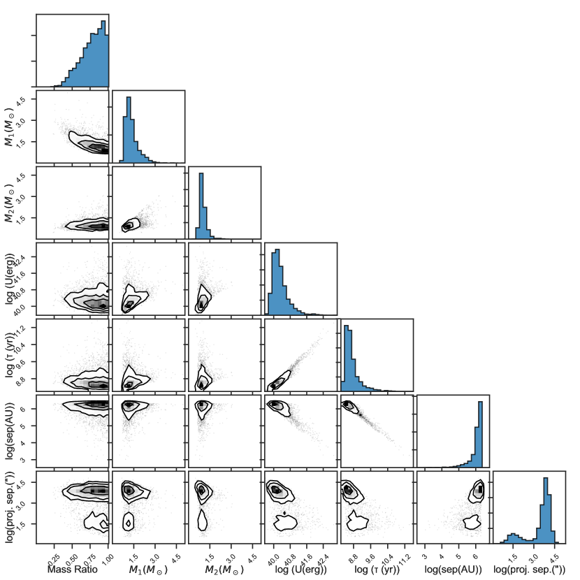
Figure 12: A corner plot summary of the mass properties of binaries in our study. We show the mass ratio, primary and secondary masses in solar masses, binding energy in ergs (log scale), binary lifetime in Gyr (log scale), physical separation in AU (log scale), and projected separation in arcseconds (log scale). The most tightly bound, and longest lived systems are found close to each other.

Figure 13: Left Panels: Binding Energy vs Total Mass for binaries in our sample. Right Panels: Binding Energy vs Separation for the same binaries. The upper panels have points shaded by dissipation timescales, which approximates how long the binary should remain gravitationally bound. The lower panels have points shaded by separation (in pc) and total mass (in $M_{\odot}$). The longest lived binaries in our sample are seen with small separations, and not necessarily large total masses. At the largest separations ($>10^{6}$ AU), there is a preference for larger total masses, suggesting that some of these widely separated pairs may be truly bound. Overall, most of the sample consists of weakly bound systems ($U\sim 10^{40}$ ergs), suggesting they are easily disrupted. These systems may have been more tightly bound in the past, but have since drifted apart due to gravitational interactions with neighboring stars or the Galactic tides.

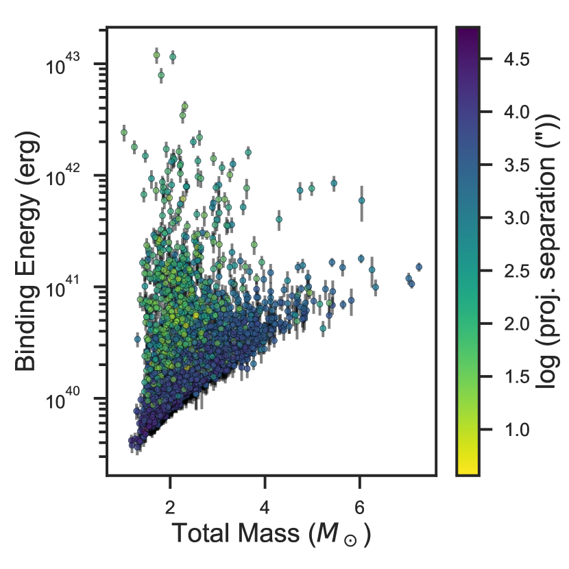
Figure 14: Binding Energy vs. Total Mass, shaded by projected separation (log scale, in arcseconds). While the trends seen in Figure 13 are not as apparent, the pairs with the largest binding energies are also found at the smallest projected separations.

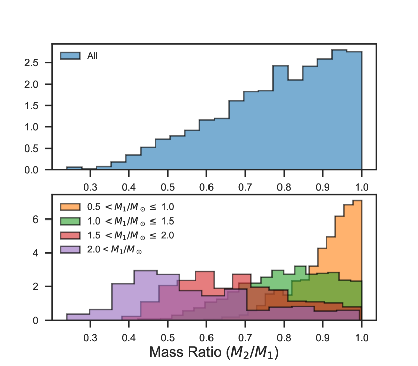
Figure 15: Upper Panel: Mass ratio histogram for stars in our sample. Lower Panel: Mass ratio distribution for various bins in primary mass. As the mass of the primary increases, the mass ratio distribution moves away from unity to increasingly flatter distributions, indicating that the secondary masses are drawn from the same distribution as the primary.

5 Conclusions

We analyzed a sample of 9,995 co-moving stars identified in $Gaia$-TGAS by Oh et al. (2017b) and reorganized by Faherty et al. (2018). Our analysis used isochrone fitting incorporating $G,J,H,K$ and $W1$ observed photometry. Our results demonstrated robust estimates of stellar masses, as verified by comparisons to other analyses of the same stars, cluster properties and computation of the PDMF. We report fundamental parameters for all stars in the sample, and examined the binary properties of pairs in the system. Many pairs in the catalog are weakly bound, sharing binding energies comparable to Neptune and the Sun (Dhital et al., 2010). The dominant property of a pair’s binding energy and lifetime is its physical separation.

This catalog, derived from the exquisite astrometry of $Gaia$ has revealed a large population of loosely bound systems, which will be ideal for large spectroscopic follow-up (i.e., Price-Whelan et al., 2017). Future samples of co-moving stars in $Gaia$ will likely be dominated by loosely bound systems, making spectroscopic observations critically important. Spectra readily reveals the radial velocity of a star, allowing for the direct comparison of a star’s 3d velocity vector to any companion. Furthermore, spectra can be used to precisely estimate stellar chemical composition, which is uncertain with photometric techniques. However, to address the significant age uncertainties, other techniques, like gyrochronology (Douglas et al., 2014, i.e.,) or astroseismology (Chaplin et al., 2014) are likely required.

References

- Andrews et al. (2017) Andrews, J. J., Chanamé, J., & Agüeros, M. A. 2017, ArXiv e-prints, arXiv:1704.07829 [astro-ph.SR]
- Astropy Collaboration et al. (2013) Astropy Collaboration, Robitaille, T. P., Tollerud, E. J., et al. 2013, A&A, 558, A33
- Bahcall et al. (1985) Bahcall, J. N., Hut, P., & Tremaine, S. 1985, ApJ, 290, 15
- Barrado y Navascués et al. (2004) Barrado y Navascués, D., Stauffer, J. R., & Jayawardhana, R. 2004, ApJ, 614, 386
- Blaauw (1946) Blaauw, A. 1946, Publications of the Kapteyn Astronomical Laboratory Groningen, 52, 1
- Bochanski et al. (2010) Bochanski, J. J., Hawley, S. L., Covey, K. R., et al. 2010, AJ, 139, 2679
- Bovy (2016) Bovy, J. 2016, ApJ, 817, 49
- Bovy (2017) —. 2017, MNRAS, 470, 1360
- Casagrande et al. (2011) Casagrande, L., Schönrich, R., Asplund, M., et al. 2011, A&A, 530, A138
- Chaplin et al. (2014) Chaplin, W. J., Basu, S., Huber, D., et al. 2014, ApJS, 210, 1
- Choi et al. (2016) Choi, J., Dotter, A., Conroy, C., et al. 2016, ApJ, 823, 102
- Crawford & Barnes (1974) Crawford, D. L., & Barnes, J. V. 1974, AJ, 79, 687
- Cummings (1921) Cummings, E. E. 1921, PASP, 33, 214
- Cummings et al. (2017) Cummings, J. D., Deliyannis, C. P., Maderak, R. M., & Steinhauer, A. 2017, AJ, 153, 128
- Cutri & et al. (2013) Cutri, R. M., & et al. 2013, VizieR Online Data Catalog, 2328
- de Zeeuw et al. (1999) de Zeeuw, P. T., Hoogerwerf, R., de Bruijne, J. H. J., Brown, A. G. A., & Blaauw, A. 1999, AJ, 117, 354
- Dhital et al. (2010) Dhital, S., West, A. A., Stassun, K. G., & Bochanski, J. J. 2010, AJ, 139, 2566
- Dhital et al. (2012) Dhital, S., West, A. A., Stassun, K. G., et al. 2012, AJ, 143, 67
- Dhital et al. (2015) Dhital, S., West, A. A., Stassun, K. G., Schluns, K. J., & Massey, A. P. 2015, AJ, 150, 57
- Dotter (2016) Dotter, A. 2016, ApJS, 222, 8
- Douglas et al. (2014) Douglas, S. T., Agüeros, M. A., Covey, K. R., et al. 2014, ApJ, 795, 161
- Elliott et al. (2016) Elliott, P., Bayo, A., Melo, C. H. F., et al. 2016, A&A, 590, A13
- ESA (1997) ESA, ed. 1997, ESA Special Publication, Vol. 1200, The HIPPARCOS and TYCHO catalogues. Astrometric and photometric star catalogues derived from the ESA HIPPARCOS Space Astrometry Mission
- Faherty et al. (2018) Faherty, J., et al. 2018, AJ, submitted
- Fitzpatrick (1999) Fitzpatrick, E. L. 1999, PASP, 111, 63
- Foreman-Mackey (2016) Foreman-Mackey, D. 2016, The Journal of Open Source Software, 2016
- Foreman-Mackey et al. (2013) Foreman-Mackey, D., Hogg, D. W., Lang, D., & Goodman, J. 2013, PASP, 125, 306
- Gagné et al. (2017a) Gagné, J., Faherty, J. K., Mamajek, E. E., et al. 2017a, ApJS, 228, 18
- Gagné et al. (2017b) Gagné, J., Faherty, J. K., Burgasser, A. J., et al. 2017b, ApJ, 841, L1
- Gagné et al. (2018) Gagné, J., Mamajek, E. E., Malo, L., et al. 2018, ArXiv e-prints, arXiv:1801.09051 [astro-ph.SR]
- Gaia Collaboration et al. (2016a) Gaia Collaboration, Brown, A. G. A., Vallenari, A., et al. 2016a, A&A, 595, A2
- Gaia Collaboration et al. (2016b) Gaia Collaboration, Prusti, T., de Bruijne, J. H. J., et al. 2016b, A&A, 595, A1
- Høg et al. (2000) Høg, E., Fabricius, C., Makarov, V. V., et al. 2000, A&A, 355, L27
- Hunter (2007) Hunter, J. D. 2007, Computing In Science & Engineering, 9, 90
- Hurley et al. (2002) Hurley, J. R., Tout, C. A., & Pols, O. R. 2002, MNRAS, 329, 897
- Ivezić et al. (2014) Ivezić, Ž., Connolly, A., Vanderplas, J., & Gray, A. 2014, Statistics, Data Mining and Machine Learning in Astronomy (Princeton University Press)
- Jiang & Tremaine (2010) Jiang, Y.-F., & Tremaine, S. 2010, MNRAS, 401, 977
- Jones et al. (2001) Jones, E., Oliphant, T., Peterson, P., et al. 2001, SciPy: Open source scientific tools for Python, [Online]
- Kaib & Raymond (2014) Kaib, N. A., & Raymond, S. N. 2014, ApJ, 782, 60
- Kaib et al. (2013) Kaib, N. A., Raymond, S. N., & Duncan, M. 2013, Nature, 493, 381
- Knuth (2006) Knuth, K. H. 2006, ArXiv Physics e-prints, physics/0605197
- Law et al. (2010) Law, N. M., Dhital, S., Kraus, A., Stassun, K. G., & West, A. A. 2010, ApJ, 720, 1727
- Lindegren et al. (2016) Lindegren, L., Lammers, U., Bastian, U., et al. 2016, A&A, 595, A4
- Mädler et al. (2016) Mädler, T., Jofré, P., Gilmore, G., et al. 2016, A&A, 595, A59
- Mainzer et al. (2011) Mainzer, A., Bauer, J., Grav, T., et al. 2011, ApJ, 731, 53
- Mamajek et al. (2002) Mamajek, E. E., Meyer, M. R., & Liebert, J. 2002, AJ, 124, 1670
- Michalik et al. (2015) Michalik, D., Lindegren, L., & Hobbs, D. 2015, A&A, 574, A115
- Morton (2015) Morton, T. D. 2015, isochrones: Stellar model grid package, Astrophysics Source Code Library, ascl:1503.010
- Netopil et al. (2016) Netopil, M., Paunzen, E., Heiter, U., & Soubiran, C. 2016, A&A, 585, A150
- Oelkers et al. (2017) Oelkers, R. J., Stassun, K. G., & Dhital, S. 2017, AJ, 153, 259
- Oh et al. (2017a) Oh, S., Price-Whelan, A. M., Brewer, J. M., et al. 2017a, ArXiv e-prints, arXiv:1709.05344 [astro-ph.SR]
- Oh et al. (2017b) Oh, S., Price-Whelan, A. M., Hogg, D. W., Morton, T. D., & Spergel, D. N. 2017b, AJ, 153, 257
- Opik (1976) Opik, E. J. 1976, Interplanetary encounters : close-range gravitational interactions
- Paxton et al. (2011) Paxton, B., Bildsten, L., Dotter, A., et al. 2011, ApJS, 192, 3
- Paxton et al. (2013) Paxton, B., Cantiello, M., Arras, P., et al. 2013, ApJS, 208, 4
- Paxton et al. (2015) Paxton, B., Marchant, P., Schwab, J., et al. 2015, ApJS, 220, 15
- Pecaut et al. (2012) Pecaut, M. J., Mamajek, E. E., & Bubar, E. J. 2012, ApJ, 746, 154
- Perryman et al. (1998) Perryman, M. A. C., Brown, A. G. A., Lebreton, Y., et al. 1998, A&A, 331, 81
- Price-Whelan et al. (2017) Price-Whelan, A. M., Oh, S., & Spergel, D. N. 2017, ArXiv e-prints, arXiv:1709.03532 [astro-ph.SR]
- Raghavan et al. (2010) Raghavan, D., McAlister, H. A., Henry, T. J., et al. 2010, ApJS, 190, 1
- Reid et al. (2002) Reid, I. N., Gizis, J. E., & Hawley, S. L. 2002, AJ, 124, 2721
- Rojas-Ayala et al. (2012) Rojas-Ayala, B., Covey, K. R., Muirhead, P. S., & Lloyd, J. P. 2012, ApJ, 748, 93
- Salpeter (1955) Salpeter, E. E. 1955, ApJ, 121, 161
- Schlafly & Finkbeiner (2011) Schlafly, E. F., & Finkbeiner, D. P. 2011, ApJ, 737, 103
- Schlegel et al. (1998) Schlegel, D. J., Finkbeiner, D. P., & Davis, M. 1998, ApJ, 500, 525
- Skrutskie et al. (2006) Skrutskie, M. F., Cutri, R. M., Stiening, R., et al. 2006, AJ, 131, 1163
- Stauffer et al. (1989) Stauffer, J., Hamilton, D., Probst, R., Rieke, G., & Mateo, M. 1989, ApJ, 344, L21
- Taylor (2005) Taylor, M. B. 2005, in Astronomical Society of the Pacific Conference Series, Vol. 347, Astronomical Data Analysis Software and Systems XIV, ed. P. Shopbell, M. Britton, & R. Ebert, 29
- Thomas et al. (2016) Thomas, K., Benjamin, R.-K., Fernando, P., et al. 2016, Stand Alone, 0, 87–90
- van der Walt et al. (2011) van der Walt, S., Colbert, S. C., & Varoquaux, G. 2011, Computing in Science Engineering, 13, 22
- van Leeuwen (2007) van Leeuwen, F. 2007, A&A, 474, 653
- van Leeuwen (2009) —. 2009, A&A, 497, 209
- Vanderplas et al. (2012) Vanderplas, J., Connolly, A., Ivezić, Ž., & Gray, A. 2012, in Conference on Intelligent Data Understanding (CIDU), 47
- VanderPlas et al. (2014) VanderPlas, J., Fouesneau, M., & Taylor, J. 2014, AstroML: Machine learning and data mining in astronomy, Astrophysics Source Code Library, ascl:1407.018
- Weinberg et al. (1986) Weinberg, M. D., Shapiro, S. L., & Wasserman, I. 1986, Icarus, 65, 27
- Weinberg et al. (1987) —. 1987, ApJ, 312, 367
- Wright et al. (2010) Wright, E. L., Eisenhardt, P. R. M., Mainzer, A. K., et al. 2010, AJ, 140, 1868