$\bar{B}^{0}$, $\bar{B}^{0}_{s}$ and $B^{-}$ decays into $\eta_{c}$ plus a scalar meson

Abstract

We investigate the decays of $\bar{B}^{0}_{s}$, $\bar{B}^{0}$ and $B^{-}$ into $\eta_{c}$ plus a scalar meson in a theoretical framework by taking into account the dominant process for the weak decay of $\bar{B}$ meson into $\eta_{c}$ and a $q\bar{q}$ pair. After hadronization of this $q\bar{q}$ component into pairs of pseudoscalar mesons we obtain certain weights for the pseudoscalar meson-pseudoscalar meson components. The calculation is based on the postulation that the scalar mesons $f_{0}(500)$, $f_{0}(980)$ and $a_{0}(980)$ are dynamically generated states from the pseudoscalar meson-pseudoscalar meson interactions in $S$-wave. Up to a global normalization factor, the $\pi\pi$, $K\bar{K}$ and $\pi\eta$ invariant mass distributions for the decays of $\bar{B}^{0}_{s}\to\eta_{c}\pi^{+}\pi^{-}$, $\bar{B}^{0}_{s}\to\eta_{c}K^{+}K^{-}$, $\bar{B}^{0}\to\eta_{c}\pi^{+}\pi^{-}$, $\bar{B}^{0}\to\eta_{c}K^{+}K^{-}$, $\bar{B}^{0}\to\eta_{c}\pi^{0}\eta$, $B^{-}\to\eta_{c}K^{0}K^{-}$ and $B^{-}\to\eta_{c}\pi^{-}\eta$ are predicted. Comparison is made with the limited experimental information available and other theoretical calcualtions. Further comparison of these results with coming LHCb measurements will be very valuable to make progress in our understanding of the nature of the low lying scalar mesons, $f_{0}(500),f_{0}(980)$ and $a_{0}(980)$.

I Introduction

In addition to the measurement of the $B^{0}_{s}\to J/\psi\pi^{+}\pi^{-}$ decay Aaij:2011fx , the branching fractions ${\rm Br}(B^{0}_{s}\to\eta_{c}\pi^{+}\pi^{-})=(1.76\pm 0.59\pm 0.12\pm 0.29)\times 10^{-4}$ and ${\rm Br}(B^{0}_{s}\to\eta_{c}\phi)=(5.01\pm 0.53\pm 0.27\pm 0.63)\times 10^{-4}$ are recently measured by the LHCb collaboration Aaij:2017hfc . The $f_{0}(980)$ is produced in the $\bar{B}^{0}_{s}$ decays into $J/\psi$ and $\pi^{+}\pi^{-}$ and no trace of the $f_{0}(500)$ is seen Aaij:2011fx , while in the $\bar{B}^{0}\to J/\psi\pi^{+}\pi^{-}$ decay, the main contribution is from the $f_{0}(500)$ with a small fraction for the $f_{0}(980)$ Aaij:2013zpt ; Aaij:2014siy . The new measurement in Ref. Aaij:2017hfc , suggests also that the $\pi^{+}\pi^{-}$ pair in $B^{0}_{s}\to\eta_{c}\pi^{+}\pi^{-}$ arises from the contribution of $f_{0}(980)$. To understand the new experimental measurements and search for some hints about involved physics, corresponding theoretical studies are needed.

Estimations of the branch ratios for some of these decays have been done by employing the perturbative QCD factorization approach Li:2015tja ; Li:2017obb . Also, in Ref. Ke:2017wni the decay widths of $B^{0}_{s}\to\eta_{c}f_{0}(980)$ and $B^{0}_{s}\to\eta_{c}\phi$ were evaluated in the light-front quark model. The conclusions of Ref. Ke:2017wni are that the mostly dominant contribution for the $B^{0}_{s}\to\eta_{c}\pi^{+}\pi^{-}$ decay is from the $f_{0}(980)$ and the $f_{0}(980)$ should be a $K\bar{K}$ molecule or a tetraquark state, at least its pure quark-antiquark component is small.

For the $B^{0}_{s}\to J/\psi\pi^{+}\pi^{-}$ decay, a simple theoretical method based on the final state interaction of mesons provided by the chiral unitary approach has been applied in Ref. Liang:2014tia , where the theoretical results are in agreement with the data. The work of Ref. Liang:2014tia isolates the dominant weak decay mechanism into $J/\psi$ and a $q\bar{q}$ pair. Then, the $q\bar{q}$ pair is hadronized, and meson-meson pars are formed with a certain weight. The final state interaction of the meson-meson components, described in the terms of chiral unitary theory, gives rise to the $f_{0}(980)$ and $f_{0}(500)$ resonances. The approach of Ref. Liang:2014tia was succesfully extended to study other weak $B$ and $D$ decays in Refs. Bayar:2014qha ; Xie:2014tma ; Xie:2014gla ; Liang:2014ama ; Liang:2015qva ; Dai:2015bcc ; Albaladejo:2016hae ; Molina:2016pbg (see also Ref. Oset:2016lyh for an extensive review). Other theoretical work has also been done within the perturbative QCD approach in Ref. Wang:2015uea . Recently, another approach has been used in Ref. Daub:2015xja using effective Hamiltonians, transversity form factors and implementing the meson-meson final sate interaction. In addition to the $\pi^{+}\pi^{-}$ production, the $\bar{B}^{0}_{s}$ decay into $J/\psi$ and $K^{+}K^{-}$ is also studied and compared to experimental measurements in Ref. Daub:2015xja .

Following this line of research, the purpose of this paper is to investigate the decays of $\bar{B}^{0}$, $\bar{B}^{0}_{s}$ and $B^{-}$ decays into $\eta_{c}$ plus a scalar meson. We evaluate the $\pi^{+}\pi^{-}$ and $K^{+}K^{-}$ invariant mass distributions in the $\bar{B}^{0}_{s}$ decays into $\eta_{c}\pi^{+}\pi^{-}$ and $\eta_{c}K^{+}K^{-}$ and the $K^{+}K^{-}$ and $\pi\eta$ production in the $\bar{B}^{0}$ decay into $\eta_{c}$ and this pair of mesons. At the same time, we investigate also the $B^{-}\to\eta_{c}K^{0}K^{-}$ and $B^{-}\to\eta_{c}\pi^{-}\eta$ decays. Up to a global factor, one can compare the strength of those invariant mass distributions.

To end this introduction, we would like to mention that, up to an arbitrary normalization, one can obtain the invariant mass distributions and relate the different mass distributions with no parameters fitted to the data. This is due to the unified picture that the chiral unitary approach provides for the final state interaction of mesons. In this sense, predictions on the coming measurements should be most welcome, and if supported by experiment, it can give us more information about the nature of these low lying scalar mesons, $f_{0}(500)$, $f_{0}(980)$ and $a_{0}(980)$, which are dynamically generated states from the interaction of pseudoscalar mesons using a meson-meson interaction derived from the chiral Lagrangians Gasser:1983yg ; Bernard:1995dp .

This article is organized as follows. In Sec. II, we present the theoretical formalism of the decays of $\bar{B}^{0}$, $\bar{B}^{0}_{s}$ and $B^{-}$ decays into $\eta_{c}$ plus a scalar meson, explaining in detail the hadronization and final state interactions of the meson-meson pairs. Numerical results and discussions are presented in Sec. III, followed by a summary in the last section.

II Formalism and ingredients

The leading contributions to the decays of $\bar{B}^{0}_{s}$, $\bar{B}^{0}$ and $B^{-}$ into $\eta_{c}$ plus a scalar meson is the $b\to c\bar{c}s$ process. In the following we will discuss the production mechanisms for these decays.

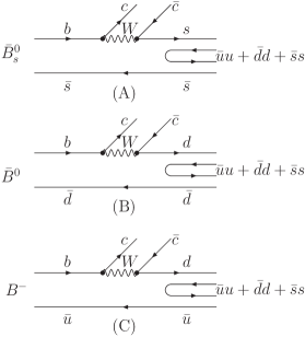
Figure 1: Diagrams for the decay of $\bar{B}^{0}$, $\bar{B}^{0}_{s}$ and $B^{-}$ into $\eta_{c}$ ($c\bar{c}$) and a primary $q\bar{q}$ pair, $s\bar{s}$ for $\bar{B}^{0}_{s}$ [(A)], $d\bar{d}$ for $\bar{B}^{0}$ [(B)], and $d\bar{u}$ for $B^{-}$ [(C)]. The schematic representation of the hadronization $\bar{q}q\to\bar{q}q(\bar{u}u+\bar{d}d+\bar{s}s)$ is also shown.

Following Refs. Liang:2014tia ; Stone:2013eaa , in Fig. 1 we show the diagrams at the quark level that are responsible for the $\bar{B}^{0}_{s}$, $\bar{B}^{0}$, and $B^{-}$ decays into $\eta_{c}$ and another pair of quarks: $s\bar{s}$ in the case of the $\bar{B}^{0}_{s}$ decay [Fig. 1 (A)], $d\bar{d}$ in the case of $\bar{B}^{0}$ decay [Fig. 1 (B)], and $d\bar{u}$ for the $B^{-}$ decay [Fig. 1 (C)]. The $\bar{B}^{0}_{s}$ decay involves the $V_{cs}$, Cabibbo favored Cabibbo-Kobayashi-Maskawa matrix element, and the $\bar{B}^{0}$ and $B^{-}$ decays involves the $V_{cd}$ Cabibbo suppressed one, which makes the widths large in the $\bar{B}^{0}_{s}$ case compared to the $\bar{B}^{0}$ and $B^{-}$ decays. 

In order to produce two mesons the $q\bar{q}$ pair has to hadronize, which one can implement adding an extra $\bar{q}q$ pair with the quantum numbers of the vacuum, $\bar{u}u+\bar{d}d+\bar{s}s$, see also in Fig. 1. Next step corresponds to writing the $q\bar{q}(\bar{u}u+\bar{d}d+\bar{s}s)$ combination in terms of pairs of mesons. Following the work of Ref. Liang:2014tia we obtain

$$d\bar{d}(\bar{u}u+\bar{d}d+\bar{s}s) \equiv\pi^{-}\pi^{+}+\frac{1}{2}\pi^{0}\pi^{0}+\frac{1}{3}\eta\eta$$ (1)

$$-\frac{2}{\sqrt{6}}\pi^{0}\eta+\bar{K}^{0}K^{0},$$

$$s\bar{s}(\bar{u}u+\bar{d}d+\bar{s}s) \equiv K^{-}K^{+}+\bar{K}^{0}K^{0}+\frac{1}{3}\eta\eta,$$ (2)

$$d\bar{u}(\bar{u}u+\bar{d}d+\bar{s}s) \equiv\frac{2}{\sqrt{3}}\pi^{-}\eta+K^{0}K^{-},$$ (3)

where the $\eta^{\prime}$ terms have been neglected because the $\eta^{\prime}$ has large mass and has very small effect here.

After the production of a meson-meson (MM) pair, the final state interaction between the meson and meson takes place, which can be parameterized by the re-scattering shown in Fig. 2 at the hadronic level. Since we consider only the $S$-wave interaction between the pseudo-scalar meson and pseudo-scalar meson, we will have the contributions from only the scalar mesons. In Fig. 2, we also show the tree level diagrams for the $\pi\pi$, $K\bar{K}$ and $\pi\eta$ production.

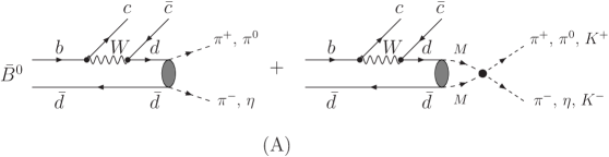
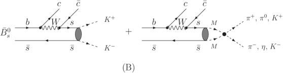
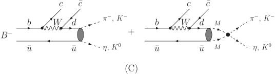
Figure 2: Diagrammatic representations of the production of $\pi^{+}\pi^{-}$, $\pi^{0}\eta$, $K^{+}K^{-}$, $\pi^{-}\eta$, and $K^{-}K^{0}$ via direct plus re-scattering mechanisms in $\bar{B}^{0}$ (A), $\bar{B}^{0}_{s}$ (B) and $B^{-}$ (C) decays.

The decay amplitudes for a final production of the different meson pairs are given by Oller:1997yg

$$T(\bar{B}^{0}_{s}\to\eta_{c}\pi^{+}\pi^{-})=V_{P}V_{cs}(G_{K^{+}K^{-}}t_{K^{+}K^{-}\to\pi^{+}\pi^{-}}$$

$$+G_{K^{0}\bar{K}^{0}}t_{K^{0}\bar{K}^{0}\to\pi^{+}\pi^{-}}+\frac{1}{3}G_{\eta\eta}t_{\eta\eta\to\pi^{+}\pi^{-}}),$$ (4)

$$T(\bar{B}^{0}_{s}\to\eta_{c}K^{+}K^{-})=V_{P}V_{cs}(1+G_{K^{+}K^{-}}t_{K^{+}K^{-}\to K^{+}K^{-}}$$

$$+G_{K^{0}\bar{K}^{0}}t_{K^{0}\bar{K}^{0}\to K^{+}K^{-}}+\frac{1}{3}G_{\eta\eta}t_{\eta\eta\to K^{+}K^{-}}),$$ (5)

$$T(\bar{B}^{0}\to\eta_{c}\pi^{+}\pi^{-})=V_{P}V_{cd}(1+G_{\pi^{+}\pi^{-}}t_{\pi^{+}\pi^{-}\to\pi^{+}\pi^{-}}$$

$$+\frac{1}{2}G_{\pi^{0}\pi^{0}}t_{\pi^{0}\pi^{0}\to\pi^{+}\pi^{-}}+G_{K^{0}\bar{K}^{0}}t_{K^{0}\bar{K}^{0}\to\pi^{+}\pi^{-}}$$

$$+\frac{1}{3}G_{\eta\eta}t_{\eta\eta\to\pi^{+}\pi^{-}}),$$ (6)

$$T(\bar{B}^{0}\to\eta_{c}\pi^{0}\eta)=V_{P}V_{cd}(-\frac{2}{\sqrt{6}}-\frac{2}{\sqrt{6}}G_{\pi^{0}\eta}t_{\pi^{0}\eta\to\pi^{0}\eta}$$

$$+G_{K^{0}\bar{K}^{0}}t_{K^{0}\bar{K}^{0}\to\pi^{0}\eta}),$$ (7)

$$T(\bar{B}^{0}\to\eta_{c}K^{+}K^{-})=V_{P}V_{cd}(G_{\pi^{+}\pi^{-}}t_{\pi^{+}\pi^{-}\to K^{+}K^{-}}$$

$$+\frac{1}{2}G_{\pi^{0}\pi^{0}}t_{\pi^{0}\pi^{0}\to K^{+}K^{-}}+\frac{1}{3}G_{\eta\eta}t_{\eta\eta\to K^{+}K^{-}}$$

$$-\frac{2}{\sqrt{6}}G_{\pi^{0}\eta}t_{\pi^{0}\eta\to K^{+}K^{-}}+G_{K^{0}\bar{K}^{0}}t_{K^{0}\bar{K}^{0}\to K^{+}K^{-}}),$$ (8)

$$T(B^{-}\to\eta_{c}\pi^{-}\eta)=V_{P}V_{cd}(\frac{2}{\sqrt{3}}+\frac{2}{\sqrt{3}}G_{\pi^{-}\eta}t_{\pi^{-}\eta\to\pi^{-}\eta}$$

$$+G_{K^{0}K^{-}}t_{K^{0}K^{-}\to\pi^{-}\eta}),$$ (9)

$$T(B^{-}\to\eta_{c}K^{0}K^{-})=V_{P}V_{cd}(1+G_{K^{0}K^{-}}t_{K^{0}K^{-}\to K^{0}K^{-}}$$

$$+\frac{2}{\sqrt{3}}G_{\pi^{-}\eta}t_{\pi^{-}\eta\to K^{0}K^{-}}).$$ (10)

where $V_{P}$ is the production vertex which contains all dynamical factors common to all the above seven decays. We shall assume $V_{P}$ as constant and fit it to the experimental date. The $G_{\rm MM}$ are the loop functions of two meson propagators. The $t_{{\rm MM}\to{\rm MM}}$ are the scattering matrices and they are calculated in Ref. Liang:2014tia following Ref. Oller:1997ti . Note that we can easily obatin $t_{\pi^{-}\eta\to\pi^{-}\eta}$, $t_{K^{0}K^{-}\to K^{0}K^{-}}$ and $t_{\pi^{-}\eta\to K^{0}K^{-}}$ using isospin symmetry,

$$t_{\pi^{-}\eta\to\pi^{-}\eta} = t_{\pi^{0}\eta\to\pi^{0}\eta},$$ (11)

$$t_{K^{0}K^{-}\to\pi^{-}\eta} = -\sqrt{2}~{}t_{K^{0}\bar{K}^{0}\to\pi^{0}\eta},$$ (12)

$$t_{K^{0}K^{-}\to K^{0}K^{-}} = \!\!t_{K^{+}K^{-}\to K^{+}K^{-}}\!-\!t_{K^{+}K^{-}\to K^{0}\bar{K}^{0}}.$$ (13)

With all the ingredients obtained in the previous section, one can write down the invariant mass distributions for those decays as

$$\frac{d\Gamma}{dM_{\rm inv}}=\frac{1}{(2\pi)^{3}}\frac{1}{4M_{\bar{B}_{j}}^{2}}p_{\eta_{c}}\tilde{p}_{\rm M}\sum\left|T\right|^{2},$$ (14)

where $M_{\bar{B}_{j}}$ is the mass of $\bar{B}^{0}$, $\bar{B}^{0}_{s}$, or $B^{-}$, while $M_{\rm inv}$ is the invariant mass of the final ${\rm MM}$ pair. The $p_{\eta_{c}}$ is the $\eta_{c}$ momentum in the rest frame of $\bar{B}_{j}$ and $\tilde{p}_{M}$ is the momentum of one pseudo-scalar meson in the rest frame of ${\rm MM}$ pair.

III Numerical Results and discussions

Same to the $\bar{B}^{0}_{s}\to J/\psi\pi^{+}\pi^{-}$ decay Liang:2014tia , the $\bar{B}^{0}_{s}\to\eta_{c}\pi^{+}\pi^{-}$ decay is also dominant by $f_{0}(980)$. In Ref. Li:2015tja , the fraction for the $f_{0}(980)$ contribution in the $\bar{B}^{0}_{s}\to\eta_{c}\pi^{+}\pi^{-}$ decay is around $70\%$. Thus, we assume 

$$\frac{{\rm Br}[\bar{B}^{0}_{s}\to\eta_{c}f_{0}(980)\to\eta_{c}\pi^{+}\pi^{-}]}{{\rm Br}(\bar{B}^{0}_{s}\to\eta_{c}\pi^{+}\pi^{-})}=(80\pm 10)\%,$$

from where we get ${\rm Br}[\bar{B}^{0}_{s}\to\eta_{c}f_{0}(980)\to\eta_{c}\pi^{+}\pi^{-}]=(1.41\pm 0.56)\times 10^{-4}$, where we have added in quadrature the three sets of errors quoted in Ref. Aaij:2017hfc .

On the other hand, if we integrated the Eq. (14), up to one free parameter $V_{P}$, we can extract the contribution from $f_{0}(980)$ for the decay of $\bar{B}^{0}_{s}\to\eta_{c}\pi^{+}\pi^{-}$, since, in our production mechanism, the main contribution for this decay is $f_{0}(980)$. Then, one can determine $V_{P}$. With $V_{cs}=0.97427$, we get

$$V_{P}=(3.44\pm 0.68)\times 10^{-6}.$$ (15)

Our theoretical results with $V_{cd}=-0.22534$ and $V_{P}=3.44\times 10^{-6}$ are summarized in Figs. 3, 4, and 5. In Fig. 3 we show the $\pi^{+}\pi^{-}$ and $K^{+}K^{-}$ invariant mass distributions for the $\bar{B}^{0}_{s}\to\eta_{c}\pi^{+}\pi^{-}$ and $\bar{B}^{0}_{s}\to\eta_{c}K^{+}K^{-}$, respectively. As one can see, the $f_{0}(980)$ production is clearly dominant while there is no evident signal for the $f_{0}(500)$. For the $\bar{B}^{0}_{s}\to\eta_{c}K^{+}K^{-}$ decay, the $K^{+}K^{-}$ distribution gets maximum strength just above the $K^{+}K^{-}$ threshold and then falls down gradually. This is due to the effect of the $f_{0}(980)$ resonance below the $K\bar{K}$ threshold.  Starting from the dominant weak decay process we have $\eta_{c}$ and $s\bar{s}$ production in the $\bar{B}^{0}_{s}$ decay. Because $s\bar{s}$ pair has isospin zero, and the strong interaction hadronization conserves it. Even the $K^{+}K^{-}$ system could be $I=0$ or $1$, the process of formation guarantees that this is an $I=0$ state and the shape of the $K^{+}K^{-}$ distribution is due to the $f_{0}(980)$ with $I=0$.

Figure 3: $\pi^{+}\pi^{-}$ and $K^{+}K^{-}$ invariant mass distributions for $\bar{B}_{s}^{0}\to\eta_{c}\pi^{+}\pi^{-}$ and $\eta_{c}K^{+}K^{-}$.

The strength for the $K^{+}K^{-}$ distribution is small compared to the one of the $f_{0}(980)$ at its peak for the $\pi^{+}\pi^{-}$ distribution, but the integrated strength over the invariant mass of $K^{+}K^{-}$ is of the same order of magnitude as that for the strength below the peak of the $f_{0}(980)$ going to $\pi^{+}\pi^{-}$. On the other hand, we should mention that we are calculating only the $S$-wave contribution of the $K^{+}K^{-}$ distribution, hence, contributions from higher waves, such as $\phi$ ($P$-wave), $f^{\prime}_{2}(1525)$ ($D$-wave) etc, are not included. It is interesting to compare this with experiment. First by integrating the strength of the $K^{+}K^{-}$ distribution over its invariant mass, up to $M_{\rm inv}(K^{+}K^{-})=1200$ MeV,  we find a ratio

$$\frac{{\rm Br}[\bar{B}^{0}_{s}\to\eta_{c}f_{0}(980)\to\eta_{c}K^{+}K^{-}]}{{\rm Br}[\bar{B}^{0}_{s}\to\eta_{c}f_{0}(980)\to\eta_{c}\pi^{+}\pi^{-}]}=0.4.$$ (16)

Secondly, if we stick to a band of energies around the $\phi$ meson peak, $990<M_{\rm inv}(K^{+}K^{-})<1050$ MeV, as done in Ref. Aaij:2013orb for the $\bar{B}^{0}_{s}\to J/\psi K^{+}K^{-}$, we get the $S$-wave fraction

$$\frac{{\rm Br}[\bar{B}^{0}_{s}\to\eta_{c}K^{+}K^{-}](S{\rm-wave})}{{\rm Br}[\bar{B}^{0}_{s}\to\eta_{c}\phi\to\eta_{c}K^{+}K^{-}]}=(13\pm 6)\times 10^{-2},$$ (17)

where ${\rm Br}[\bar{B}^{0}_{s}\to\eta_{c}\phi]=(5.01\pm 0.87)\times 10^{-4}$ Aaij:2017hfc and the branching fraction of $0.489$ for $\phi$ decay into $K^{+}K^{-}$ has been taken Patrignani:2016xqp . This value, one of our model predictions, could be tested by future experiment.

We come back now to the decays of the $\bar{B}^{0}$. In Fig. 4 we show the theoretical results for the $\pi^{+}\pi^{-}$, $K^{+}K^{-}$ and $\pi^{0}\eta$, invariant mass distributions for $\bar{B}^{0}\to\eta_{c}\pi^{+}\pi^{-}$, $\eta_{c}K^{+}K^{-}$, and $\eta_{c}\pi^{0}\eta$. In the $\bar{B}^{0}$ decays, we had the hadronization of a $d\bar{d}$ pair, which contains $I=0$ and $1$. But, the $\pi^{+}\pi^{-}$ in $S$-wave can only be in $I=0$, hence the peaks for the $\pi^{+}\pi^{-}$ distribution due to the $f_{0}(500)$ and $f_{0}(980)$ excitation. It is expected that the $\rho^{0}$ contribution peaks around 770 MeV, and has larger strength than the $f_{0}(500)$ contribution, but at invariant masses around 500 MeV and bellow, the strength of the $f_{0}(500)$ dominates the one of the $\rho^{0}$ meson. For the $K^{+}K^{-}$ production in the $\bar{B}^{0}$ decay, we have considered both the $I=0$ [$f_{0}(980)$] and $I=1$ [$a_{0}(980)$] contribution.

Figure 4: $\pi^{+}\pi^{-}$, $\pi^{0}\eta$, $K^{+}K^{-}$ invariant mass distributions for $\bar{B}^{0}\to\eta_{c}\pi^{+}\pi^{-}$, $\eta_{c}K^{+}K^{-}$, $\eta_{c}\pi^{0}\eta$.

Figure 5: $\pi^{-}\eta$ and $K^{0}K^{-}$ invariant mass distributions for $B^{-}\to\eta_{c}\pi^{-}\eta$ and $B^{-}\to\eta_{c}K^{0}K^{-}$.

One can see that, from Fig. 4, the strength of the $f_{0}(980)$ excitation is very small compared to that of the $f_{0}(500)$ (the broad peak to the left). Note that because of the experimental resolution the $f_{0}(980)$ peak would not appears so narrow in the experiments. As done in Refs. Liang:2014tia ; Xie:2014tma , we can extract the $f_{0}(500)$ contribution to the branching ratio by assuming a smooth background below the $f_{0}(980)$ peak, we find

$${\rm Br}[\bar{B}^{0}\to\eta_{c}f_{0}(500)\to\eta_{c}\pi^{+}\pi^{-}]\!\!=\!\!(1.2\pm 0.5)\times 10^{-5},$$ (18)

with error from the uncertainty of $V_{P}$ shown in Eq. (15). Then we find a ratio, $R$

$$R\!\!=\!\!\frac{{\rm Br}[\bar{B}^{0}\to\eta_{c}f_{0}(500)\to\eta_{c}\pi^{+}\pi^{-}]}{{\rm Br}[\bar{B}^{0}_{s}\to\eta_{c}f_{0}(980)\to\eta_{c}\pi^{+}\pi^{-}]}\!\!=\!\!(9\pm 5)\times 10^{-2},$$ (19)

which is consistent with the ones obtained in Ref. Li:2015tja : $R=(3\sim 8)\times 10^{-2}$ in Breit-Wigner model and $R=(4\sim 12)\times 10^{-2}$ in Bugg model.  However, the branch ratio, ${\rm Br}[\bar{B}^{0}\to\eta_{c}f_{0}(500)\to\eta_{c}\pi^{+}\pi^{-}]$ obtained here, is much larger than the one obtained in Ref. Li:2015tja with the perturbative QCD factorization approach. We hope the future experimental measurements can clarify this issue.

In Fig. 4, the $\pi^{0}\eta$ invariant mass distribution has a sizeable strength, bigger than that for the $\pi^{+}\pi^{-}$ and $K^{+}K^{-}$. As one can see, we get the typical cusp structure of the $a_{0}(980)$. This prediction is tied exclusively to the weights of the starting meson meson channels in Eq. (1) and the final state interaction in Eqs. (6), (7), and (8). Hence, this is a prediction of this approach, not tied to any experimental input.

Next, we show the results for $B^{-}$ decay in Fig. 5, where the strength for the $\pi^{-}\eta$ invariant mass distribution is two times as big as the one of $\bar{B}^{0}\to\eta_{c}\pi^{0}\eta$ shown in Fig. 4. For the $K^{0}K^{-}$ mass distribution we see that the position of the peak has moved to higher invariant masses compared to the $K^{+}K^{-}$ invariant mass spectrum of the $\bar{B}^{0}\to\eta_{c}K^{+}K^{-}$ or $\bar{B}_{s}^{0}\to\eta_{c}K^{+}K^{-}$ decays. In fact, the $K^{0}K^{-}$ invariant mass distribution in the $B^{-}$ decay due to the $a_{0}(980)$, which is seen in the figures, is much wider than that of the $f_{0}(980)$. It would be most instructive to see all these features in future experiments.

IV Summary

We have performed a study of the $\pi\pi$, $\pi\eta$ and $K\bar{K}$ invariant mass distributions for $\bar{B}^{0}_{s}\to\eta_{c}\pi^{+}\pi^{-}$, $\bar{B}^{0}_{s}\to\eta_{c}K^{+}K^{-}$, $\bar{B}^{0}\to\eta_{c}\pi^{+}\pi^{-}$, $\bar{B}^{0}\to\eta_{c}K^{+}K^{-}$, $\bar{B}^{0}\to\eta_{c}\pi^{0}\eta$, $B^{-}\to\eta_{c}\pi^{-}\eta$, and $B^{-}\to\eta_{c}K^{0}K^{-}$. We take the dominant mechanism for the weak decay of the $B$ meson, going to $\eta_{c}$ and a $q\bar{q}$ pair that, upon hadronization, leads to $\pi\pi$, $\pi\eta$, and $K\bar{K}$ in the final state, and this interaction is basically mediated by the scalar mesons, $f_{0}(500)$, $f_{0}(980)$, and $a_{0}(980)$.

Up to a global factor, which is determined to the experimental measurement, we can compare the strength of the $\pi\pi$, $\pi\eta$ and $K\bar{K}$ invariant mass distributions. For the $\bar{B}^{0}_{s}\to\eta_{c}K^{+}K^{-}$, only the $f_{0}(980)$ resonance contributes to the $K^{+}K^{-}$ mass distribution, but in the case of the $\bar{B}^{0}\to\eta_{c}K^{+}K^{-}$, both the $f_{0}(980)$ and $a_{0}(980)$ resonances contribute to its strength. The strength of the $K\bar{K}$ invariant mass distribution in the $\bar{B}^{0}_{s}$ decay is much larger than the one in $\bar{B}^{0}$ decay, which is because the $\bar{B}^{0}_{s}$ decay is Cabibbo favored process, while the $\bar{B}^{0}$ decay is the Cabibbo suppressed process. In the case of the $\bar{B}^{0}\to\eta_{c}\pi^{0}\eta$, one finds a cusp structure for the $a_{0}(980)$ and its strength is much larger than the one for the $\bar{B}^{0}\to\eta_{c}\pi^{+}\pi^{-}$ decay around the $f_{0}(980)$ peak.

Our theoretical results shown here are predictions for ongoing experiments at LHCb, and comparison of the observed results with our predictions will be most useful to make progress in our understanding of the meson-meson interaction and the nature of the low lying scalar mesons.

References

[1]
R. Aaij et al. [LHCb Collaboration],
Phys. Lett. B 698, 115 (2011).
[2]
R. Aaij et al. [LHCb Collaboration],
JHEP 1707, 021 (2017).
[3]
R. Aaij et al. [LHCb Collaboration],
Phys. Rev. D 87, 052001 (2013).
[4]
R. Aaij et al. [LHCb Collaboration],
Phys. Rev. D 90, 012003 (2014).
[5]
Y. Li, A. J. Ma, W. F. Wang and Z. J. Xiao,
Eur. Phys. J. C 76, 675 (2016).
[6]
Y. Li, A. J. Ma, Z. Rui and Z. J. Xiao,
Nucl. Phys. B 924, 745 (2017).
[7]
H. W. Ke and X. Q. Li,
Phys. Rev. D 96, 053005 (2017).
[8]
W. H. Liang and E. Oset,
Phys. Lett. B 737, 70 (2014).
[9]
M. Bayar, W. H. Liang and E. Oset,
Phys. Rev. D 90, 114004 (2014).
[10]
J. J. Xie, L. R. Dai and E. Oset,
Phys. Lett. B 742, 363 (2015).
[11]
J. J. Xie and E. Oset,
Phys. Rev. D 90, 094006 (2014).
[12]
W. H. Liang, J. J. Xie and E. Oset,
Phys. Rev. D 92, 034008 (2015).
[13]
W. H. Liang, J. J. Xie and E. Oset,
Eur. Phys. J. C 75, 609 (2015).
[14]
L. R. Dai, J. J. Xie and E. Oset,
Eur. Phys. J. C 76, 121 (2016).
[15]
M. Albaladejo, D. Jido, J. Nieves and E. Oset,
Eur. Phys. J. C 76, 300 (2016).
[16]
R. Molina, M. Döring and E. Oset,
Phys. Rev. D 93, 114004 (2016).
[17]
E. Oset et al.,
Int. J. Mod. Phys. E 25, 1630001 (2016).
[18]
W. F. Wang, H. N. Li, W. Wang and C. D. Lu,
Phys. Rev. D 91, 094024 (2015).
[19]
J. T. Daub, C. Hanhart and B. Kubis,
JHEP 1602, 009 (2016).
[20]
J. Gasser and H. Leutwyler,
Annals Phys. 158, 142 (1984).
[21]
V. Bernard, N. Kaiser and U. -G. Meißner,
Int. J. Mod. Phys. E 4, 193 (1995).
[22]
S. Stone and L. Zhang,
Phys. Rev. Lett. 111, 062001 (2013).
[23]
J. A. Oller and E. Oset,
Nucl. Phys. A 629, 739 (1998).
[24]
J. A. Oller and E. Oset,
Nucl. Phys. A 620, 438 (1997)
Erratum: [Nucl. Phys. A 652, 407 (1999)].
[25]
R. Aaij et al. [LHCb Collaboration],
Phys. Rev. D 89, 092006 (2014).
[26]
W. H. Liang, J. J. Xie and E. Oset,
Eur. Phys. J. C 76, 700 (2016).
[27]
V. R. Debastiani, W. H. Liang, J. J. Xie and E. Oset,
Phys. Lett. B 766, 59 (2017).
[28]
Z. H. Guo, L. Liu, U. G. Meißner, J. A. Oller and A. Rusetsky,
Phys. Rev. D 95, 054004 (2017).
[29]
R. Aaij et al. [LHCb Collaboration],
Phys. Rev. D 87, 072004 (2013).
[30]
C. Patrignani et al. [Particle Data Group],
Chin. Phys. C 40, 100001 (2016).
[31]
T. Sekihara and E. Oset,
Phys. Rev. D 92, 054038 (2015).