Application of a new method to study the spin equilibrium of Aql X–1: the possibility of gravitational radiation

Abstract

Accretion via disks can make neutron stars in low-mass X-ray binaries (LMXBs) fast spinning, and some of these stars are detected as millisecond pulsars. Here we report a practical way to find out if a neutron star in a transient LMXB has reached the spin equilibrium by disk–magnetosphere interaction alone, and if not, to estimate this spin equilibrium frequency. These can be done using specific measurable source luminosities, such as the luminosity corresponding to the transition between the accretion and propeller phases, and the known stellar spin rate. Such a finding can be useful to test if the spin distribution of millisecond pulsars, as well as an observed upper cutoff of their spin rates, can be explained using disk–magnetosphere interaction alone, or additional spin-down mechanisms, such as gravitational radiation, are required. Applying our method, we find that the neutron star in the transient LMXB Aql X–1 has not yet reached the spin equilibrium by disk–magnetosphere interaction alone. We also perform numerical computations, with and without gravitational radiation, to study the spin evolution of Aql X–1 through a series of outbursts and to constrain its properties. While we find that the gravitational wave emission from Aql X–1 cannot be established with certainty, our numerical results show that the gravitational radiation from Aql X–1 is possible, with a $1.6\times 10^{37}$ g cm² upper limit of the neutron star misaligned mass quadrupole moment.

1 Introduction

Millisecond pulsars (MSPs) are fast-spinning neutron stars. They are believed to attain a high spin frequency ($\nu$), typically of several hundred Hz, by accretion-induced angular momentum transfer in their low-mass X-ray binary (LMXB) phase (Radhakrishnan & Srinivasan, 1982; Alpar et al., 1982; Wijnands & van der Klis, 1998; Chakrabarty & Morgan, 1998; Archibald et al., 2009; Papitto et al., 2013; de Martino et al., 2013; Bassa et al., 2014). However, the details of such angular momentum transfer from a companion star via an accretion disk is not fully understood yet. For example, it is not clear why the spin distribution of MSPs is what it is (Watts, 2012; Patruno & Watts, 2012), and why these spin frequencies cut off above $\nu_{\rm cut}\sim 730$ Hz (Chakrabarty et al., 2003; Chakrabarty, 2005; Patruno, 2010; Ferrario & Wickramasinghe, 2007; Hessels, 2008; Papitto et al., 2014), which is well below the neutron star breakup spin rates (Cook et al., 1994; Bhattacharyya et al., 2016).

The most basic reason to explain the cutoff frequency involves the equilibrium spin frequency $\nu_{\rm eq}$, which we briefly describe here. For a spinning, magnetic neutron star, which accretes from a geometrically thin Keplerian accretion disk, the disk inner edge should be located where the rate of angular momentum removal from the disk by the stellar magnetic field begins to exceed the viscous stress. This gives the disk inner edge radius or the magnetospheric radius (e.g., Wang, 1996)

$$r_{\rm m}=\xi\left(\frac{\mu^{4}}{2GM\dot{M}^{2}}\right)^{1/7}.$$ (1)

Here, $M$ is the stellar gravitational mass (hereafter, mass), $\dot{M}$ is the accretion rate, $\mu~{}(=BR^{3})$ is the stellar magnetic dipole moment, $B$ is the stellar surface dipole magnetic field, $R$ is the stellar radius and $\xi$ is an order of unity constant. Note that $\xi$ depends on the disk–magnetosphere interaction and the magnetic pitch at the inner edge of the disk (Wang, 1996). Another important radius, the corotation radius, where the disk Keplerian angular velocity is the same as the stellar angular velocity, is given by

$$r_{\rm co}=\left(\frac{GM}{4\pi^{2}\nu^{2}}\right)^{1/3}.$$ (2)

When $r_{\rm co}>r_{\rm m}$, i.e., in the accretion phase, accretion in an LMXB happens, the neutron star spins up by a net positive torque, and $r_{\rm co}$ decreases. On the other hand, when $r_{\rm co}<r_{\rm m}$, i.e., in the so-called “propeller regime,” accreted matter is partially driven away from the system (Illarionov & Sunyaev, 1975; Ustyugova et al., 2006; D’Angelo & Spruit, 2010; Bhattacharyya & Chakrabarty, 2017) at the expense of the stellar angular momentum, resulting in a stellar spin-down by a net negative torque and an increase of $r_{\rm co}$. Therefore, $r_{\rm co}$ tends to become $r_{\rm m}$ by a self-regulated mechanism. This spin equilibrium corresponds to a frequency (obtained by $r_{\rm m}=r_{\rm co}$ condition):

$$\nu_{\rm eq}=\frac{1}{2\pi}\sqrt{\frac{GM}{r_{\rm m}^{3}}}=\frac{1}{2^{11/14}\pi\xi^{3/2}}\left(\frac{G^{5}M^{5}\dot{M}^{3}}{\mu^{6}}\right)^{1/7},$$ (3)

which is the maximum spin frequency a neutron star can attain by disk–magnetosphere interaction, and which could explain the above-mentioned observed upper cutoff frequency. Moreover, many accreting neutron stars may have already attained the $\nu_{\rm eq}$ value through the disk–magnetosphere interaction, and if so, the spin equilibrium frequency may largely explain the spin distribution of MSPs (e.g., Lamb & Yu, 2005; Patruno et al., 2012).

However, it is not certain and is a topic of current debate whether spin equilibrium due to disk–magnetosphere interaction alone can explain the spin distribution and cutoff. For example, for a high accretion rate and/or a low $B$ value, $\nu_{\rm eq}$ could be much higher than $\nu_{\rm cut}$. Therefore, a spin-down due to gravitational radiation may be required to explain the cutoff spin frequency and the spin distribution (Bildsten, 1998; Andersson et al., 1999; Chakrabarty et al., 2003). On the other hand, most of the X-ray MSPs accrete mass with a low average rate, and hence there is a possibility that their spin rates could be explained with the disk–magnetosphere interaction alone, as $\nu_{\rm eq}$ ($\propto\dot{M}^{3/7}$; see Equation 3) could be low (see, for example, Lamb & Yu, 2005). But almost all the X-ray MSPs are transient sources (Watts, 2012; Patruno & Watts, 2012), and recently Bhattacharyya & Chakrabarty (2017) have shown that a neutron star in a transient can be spun up to a frequency several times higher than that of a neutron star in a persistent source for the same long-term average $\dot{M}$. This is because, while Equation 3 works for persistent sources, a different expression of the spin equilibrium frequency should be used for transient sources. Therefore, Bhattacharyya & Chakrabarty (2017) have suggested that an additional spin-down, for example due to gravitational radiation, may be required to explain the observed spin distribution and $\nu_{\rm cut}$.

In order to test the above-mentioned possibilities for transients, it is very important to devise a way (1) to find out if a neutron star in an LMXB has reached the spin equilibrium by disk–magnetosphere interaction alone, and if not, then (2) to estimate the spin equilibrium frequency. It will be particularly useful if this method works even with a small number of known parameter values. In this paper, we provide such a method for transient LMXBs to achieve both the above-mentioned goals. We also apply this method for a prolifically outbursting transient neutron star LMXB Aql X–1 (e.g., Güngör et al., 2014). We also perform numerical computation of the evolution of Aql X–1 through a series of outbursts, and report an upper limit of the stellar misaligned mass quadrupole moment, which causes the gravitational radiation.

2 Torques and spin equilibrium for transients

Bhattacharyya & Chakrabarty (2017) have reported a crucial effect of transient accretion on the spin-up of MSPs, which was not recognized earlier. The new method presented in our paper uses this effect, and hence, in this section, we briefly discuss the torques on and spin equilibrium of neutron stars in transient systems from Bhattacharyya & Chakrabarty (2017).

In our numerical calculations, we use the following expressions of torques on a spinning neutron star due to disk–magnetosphere interaction (Rappaport et al., 2004; Bhattacharyya & Chakrabarty, 2017):

$$N=\dot{M}\sqrt{GMr_{\rm m}}+\frac{\mu^{2}}{9r_{\rm m}^{3}}\left[2\left(\frac{r_{\rm m}}{r_{\rm co}}\right)^{3}-6\left(\frac{r_{\rm m}}{r_{\rm co}}\right)^{3/2}+3\right]$$ (4)

for the accretion phase, and

$$N=-\eta\dot{M}\sqrt{GMr_{\rm m}}-\frac{\mu^{2}}{9r_{\rm m}^{3}}\left[3-2\left(\frac{r_{\rm co}}{r_{\rm m}}\right)^{3/2}\right]$$ (5)

for the propeller phase. In each expression, the first term is the material contribution, while the second term is due to the disk–magnetosphere interaction (see Bhattacharyya & Chakrabarty (2017) for derivation). In the propeller phase, for a relatively small range of $\dot{M}$ values, $r_{\rm m}$ is close to $r_{\rm co}$. For this range of $\dot{M}$, only an unknown fraction of the accreting matter could be expelled from the system, and the rest of the matter could accumulate and eventually fall on the neutron star in a cyclic manner (e.g., D’Angelo & Spruit, 2010). This could introduce some uncertainty in the numerical results, when Equation 5 is used. But note that this could happen only for a small fraction of the propeller phase duration for transients, as $\dot{M}$ evolves considerably (Bhattacharyya & Chakrabarty, 2017). Moreover, we have also checked that such a cyclic accretion for a limited time can have a small effect (at most a few percent) on the long-term spin evolution of neutron stars. Besides, the uncertainty in the material torque due to an unknown fraction of matter ejected in the propeller phase is accounted for by an order of unity positive constant $\eta$ (Equation 5; see also Bhattacharyya & Chakrabarty, 2017). Therefore, it is reasonable to use Equation 5.

For our analytical calculations, for the sake of simplicity, we use a torque expression

$$N=\frac{{\rm d}J}{{\rm d}t}=\pm A\dot{M}^{6/7},$$ (6)

which can be approximated from Equations 4 and 5, as shown in Bhattacharyya & Chakrabarty (2017). This approximation gives at most a few percent error in the spin evolution. Here $J$ and $A$ are the stellar angular momentum and a positive constant, respectively, and the positive sign corresponds to the accretion phase, while the negative sign corresponds to the propeller phase. Note that $A$ is a function of $M$, $\xi$, $B$, $R$ and a constant $\beta$, where $0\leq\beta\leq 1$ (see Equation 18 of Bhattacharyya & Chakrabarty, 2017).

In order to compare the theoretical results with observations, it is convenient to use the source luminosity $L$ instead of $\dot{M}$. It is reasonable to assume $L\propto\dot{M}$ (e.g., Patruno et al., 2012), and hence we can rewrite Equation 6 as

$$N=\frac{{\rm d}J}{{\rm d}t}=\pm\alpha L^{6/7},$$ (7)

where $\alpha$ is a function of $A$ and the proportionality constant between $L$ and $\dot{M}$. However, note that the $L-\dot{M}$ relation is expected to be somewhat different in accretion and in propeller phases (as the outburst decay profile should steepen when a source enters in the propeller phase), and hence the $L$-value of one of these phases should be suitably scaled.

Now we discuss spin equilibrium of neutron stars in transient systems by disk–magnetosphere interaction alone. Equation 3 does not give the spin equilibrium frequency for a transient accretor. This is because the $r_{\rm m}=r_{\rm co}$ condition cannot be satisfied throughout an outburst, as $\dot{M}$, and hence $r_{\rm m}$, drastically evolve. A practical way to define the spin equilibrium for a transient is by considering that no net angular momentum is transferred to the neutron star in an outburst cycle. Bhattacharyya & Chakrabarty (2017) have shown that this criterion for spin equilibrium works well for transients, as the corresponding effective spin equilibrium frequency matches within a few percent with the numerical result. As shown in Equation 20 of Bhattacharyya & Chakrabarty (2017), the criterion of ‘no net angular momentum transfer’ implies

$$L_{\rm peak}^{13/7}-L_{\rm tran,eff}^{13/7}=L_{\rm tran,eff}^{13/7}.$$ (8)

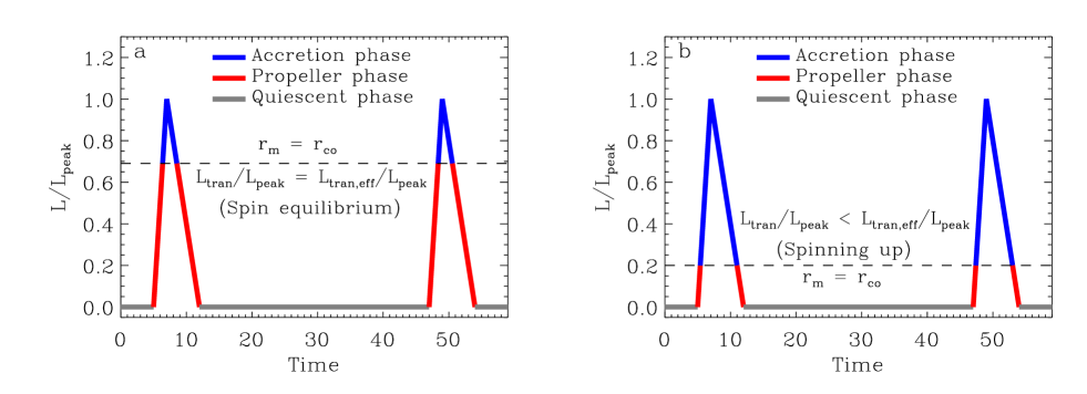
Figure 1: Schematic illustration of three phases of an outburst cycle of a transient source. Here, we assume a linear luminosity ($L$) profile with the same peak value ($L_{\rm peak}$) for each outburst. Time is given in an arbitrary unit and two outbursts are shown in each panel. Panel a is for the effective spin equilibrium of the neutron star, as the total positive angular momentum transfer to the star in the accretion phase (blue portion) balances the total negative angular momentum transfer in the propeller phase (red portion). This happens if the luminosity $L_{\rm tran}$ corresponding to the transition between accretion and propeller phases (defined by $r_{\rm m}=r_{\rm co}$) is equal to $L_{\rm tran,eff}=0.69\times L_{\rm peak}$ (see Section 2). Panel b is similar to the panel a, but here the star is still spinning up and has not yet reached the effective spin equilibrium. This happens when $L_{\rm tran}$ is less than $L_{\rm tran,eff}$ (see Section 3.1).

Here, and in Figure 1a which explains this equation, $L_{\rm peak}$ is the peak luminosity of each outburst with a linear $L$ profile, $L_{\rm tran}$ is the luminosity corresponding to the transition between accretion and propeller phases (i.e., $r_{\rm m}=r_{\rm co}$) at the present time, and $L_{\rm tran,eff}$ is the $L_{\rm tran}$ value when the effective spin equilibrium is reached. The left-hand side of Equation 8 is proportional to the stellar angular momentum gain in the accretion phase (blue portion of an outburst in Figure 1a), while the right-hand side of the same equation is proportional to the stellar angular momentum loss in the propeller phase (red portion of an outburst in Figure 1a). Equation 8 implies

$$l_{\rm eff}=\frac{L_{\rm tran,eff}}{L_{\rm peak}}=2^{-7/13}=0.69,$$ (9)

in the effective spin equilibrium, which is shown by a dashed horizontal line in Figure 1a.

Note that the luminosity $L$ and hence $r_{\rm m}$ evolve for a transient source, resulting in an equilibrium spin frequency $\nu_{\rm eq}$ value corresponding to each luminosity value during an outburst cycle (see Equation 3 and $L\propto\dot{M}$). Two such frequencies are $\nu_{\rm eq,tran,eff}$ and $\nu_{\rm eq,peak}$, which are equilibrium spin frequencies that would be obtained (using Equation 3) in case of persistent accretion corresponding to $L_{\rm tran,eff}$ and $L_{\rm peak}$ respectively. Therefore, using Equations 9 and 3 we get

$$\frac{\nu_{\rm eq,tran,eff}}{\nu_{\rm eq,peak}}=\left[\frac{L_{\rm tran,eff}}{L_{\rm peak}}\right]^{3/7}=2^{-3/13}=0.85,$$ (10)

We note that $\nu_{\rm eq,tran,eff}$, being the equilibrium spin frequency (Equation 3) corresponding to $L_{\rm tran,eff}$, is also the effective spin equilibrium frequency for a transient source, as defined in Bhattacharyya & Chakrabarty (2017). Therefore, with mass transfer, $\nu$ increases and tends to become $\nu_{\rm eq,tran,eff}$ for a transient source, as this effective spin equilibrium frequency is the maximum spin frequency a transiently accreting neutron star can attain by disk–magnetosphere interaction alone (Bhattacharyya & Chakrabarty, 2017).

We sometimes consider two additional spin-down torques in this paper. If the neutron star loses angular momentum because of the electromagnetic torque

$$N_{\rm EM}=-\frac{2\mu^{2}}{3r_{\rm lc}^{3}}=-\frac{16\pi^{3}\mu^{2}\nu^{3}}{3c^{3}}$$ (11)

due to magnetic dipole radiation during the quiescence period, the effective spin equilibrium frequency will be smaller than $\nu_{\rm eq,tran,eff}$. Here, the speed-of-light cylinder radius $r_{\rm lc}=c/2\pi\nu$. Besides, if the neutron star loses angular momentum continuously due to gravitational wave torque

$$N_{\rm GW}=-\frac{32GQ^{2}}{5}\left(\frac{2\pi\nu}{c}\right)^{5},$$ (12)

the effective spin equilibrium frequency will also be smaller than $\nu_{\rm eq,tran,eff}$. Here, $Q$ is the stellar rotating misaligned mass quadrupole moment (Bildsten, 1998).

3 A new way to test spin equilibrium in transients

3.1 For outbursts with the same peak luminosity

In this section, we use the background given in Sections 1 and 2 to describe a way to find out if a neutron star in a transient system has reached the effective spin equilibrium by disk–magnetosphere interaction alone. We assume linear luminosity profiles of outbursts with the same peak luminosity $L_{\rm peak}$ for each outburst. For our purpose, we use only one measurable parameter, i.e., the ratio of two source luminosities $l=L_{\rm tran}/L_{\rm peak}$ (see Section 2). When the effective spin equilibrium is reached, i.e., $L_{\rm tran}=L_{\rm tran,eff}$, then $l=l_{\rm eff}=L_{\rm tran,eff}/L_{\rm peak}=0.69$ (Section 2). Therefore, if the measured value of $l$ is consistent with $l_{\rm eff}$ ($=0.69$), one can conclude that the neutron star has reached the effective spin equilibrium by disk–magnetosphere interaction. Note that $l_{\rm eff}$ is the maximum value that $l$ can achieve, because the effective spin equilibrium frequency $\nu_{\rm eq,tran,eff}$ is the maximum spin frequency a neutron star can attain while spinning up via disk–magnetosphere interaction (Section 2). Therefore, a lower value of $l$ implies that a net positive angular momentum is being transferred to the neutron star (see Figure 1b) and the star is still spinning up. Hence, if the measured $l$ value is significantly less than $l_{\rm eff}$ ($=0.69$), one can conclude that the neutron star has not yet reached the effective spin equilibrium by disk–magnetosphere interaction.

Now, suppose the measured $l$ value indicates that the effective spin equilibrium has not been reached yet. How can one then estimate the effective spin equilibrium frequency $\nu_{\rm eq,tran,eff}$, if the stellar spin frequency $\nu$ is known? Note that, since $L_{\rm tran}$ is the luminosity corresponding to the transition between accretion and propeller phases (i.e., $r_{\rm m}=r_{\rm co}$) at the present time and $\nu$ is the current stellar spin frequency (see Sections 1 and 2), the equilibrium spin frequency $\nu_{\rm eq}$ (Equation 3) corresponding to $L_{\rm tran}$ is $\nu$. Therefore,

$$\nu\propto B^{-6/7}R^{-18/7}M^{5/7}L_{\rm tran}^{3/7}.$$ (13)

On the other hand (see Section 2),

$$\nu_{\rm eq,tran,eff}\propto B_{\rm eff}^{-6/7}R_{\rm eff}^{-18/7}M_{\rm eff}^{5/7}L_{\rm tran,eff}^{3/7},$$ (14)

where, $B_{\rm eff}$, $R_{\rm eff}$ and $M_{\rm eff}$ are stellar magnetic field, radius, and mass when the effective spin equilibrium is reached. Therefore,

$$\nu_{\rm eq,tran,eff}=\nu\left(\frac{B}{B_{\rm eff}}\right)^{6/7}\left(\frac{R}{R_{\rm eff}}\right)^{18/7}\left(\frac{M_{\rm eff}}{M}\right)^{5/7}\left(\frac{l_{\rm eff}}{l}\right)^{3/7}.$$ (15)

Note that, since the neutron star will reach the spin equilibrium via accretion-induced spin-up, $M_{\rm eff}>M$. Considering a neutron star mass range of $(1-2)M_{\odot}$, and a mass increase of $(0.1-0.4)M_{\odot}$ due to accretion, the range of $M_{\rm eff}/M$ is $1.05-1.4$. The fractional change of $R$ is usually much smaller than the fractional change of $M$. Therefore, it is reasonable to consider $R^{18/7}{M_{\rm eff}}^{5/7}>{R_{\rm eff}}^{18/7}M^{5/7}$. We also note that, for fast spinning neutron stars, it is reasonable to assume a fixed magnetic field strength, which is already low (Bhattacharyya & Chakrabarty, 2017). This implies $B=B_{\rm eff}$. However, even if there is a reduction of the magnetic field value due to accretion, then $B>B_{\rm eff}$. Therefore,

$$\nu_{\rm eq,tran,eff}\geq\nu(l_{\rm eff}/l)^{3/7}.$$ (16)

Thus, the ratio of two measured luminosities ($L_{\rm peak}$ and $L_{\rm tran}$) can be used to test if a neutron star has reached the effective spin equilibrium, and additionally the measured stellar spin frequency can provide a lower limit of the effective spin equilibrium frequency.

3.2 For outbursts with varying peak luminosity

In Section 3.1, we assumed the same peak luminosity $L_{\rm peak}$ for each outburst. But, in reality, $L_{\rm peak}$ can drastically vary from one outburst to another. Let us now explore how to incorporate a varying $L_{\rm peak}$ in our method.

Suppose, $L_{\rm peak}^{\rm max}$ and $L_{\rm peak}^{\rm min}$ are maximum and minimum values of $L_{\rm peak}$ respectively, and $L_{\rm peak}$ varies in this range. In this scenario, the effective spin equilibrium is reached if no net angular momentum is transferred to the neutron star during a set of large numbers of outbursts. Note that it is quite practical to define an effective spin equilibrium in this way, because given the small duraton (e.g., months) of each outburst cycle, the total duration of a large number of outbursts is much smaller compared to the spin-up time scale (typically $>10^{8}$ years; see Figures 2 and 3).

Here we write the angular momentum balance equation for a varying peak luminosity after generalizing Equation 8 by summing over a large number ($K$) of outbursts:

$$\sum_{s>l_{\rm m,eff}}\left[s^{13/7}-l_{\rm m,eff}^{13/7}\right]=\sum_{s>l_{\rm m,eff}}l_{\rm m,eff}^{13/7}+\sum_{s\leq l_{\rm m,eff}}s^{13/7}.$$ (17)

Here, $s=L_{\rm peak}/L_{\rm peak}^{\rm max}$ and $l_{\rm m,eff}=L_{\rm tran,eff}/L_{\rm peak}^{\rm max}$. Note that the left-hand side of Equation 17 is proportinal to the stellar angular momentum gain for the outbursts ($k$ in number) with $s>l_{\rm m,eff}$ (or, $L_{\rm peak}>L_{\rm tran,eff}$), for which the accretion phase exists when spin equilibrium is reached. The right-hand side of Equation 17 is proportinal to the stellar angular momentum loss in the propeller phase. Note that the second term on the right-hand side is for $(K-k)$ number of outbursts with $s\leq l_{\rm m,eff}$ ($L_{\rm peak}\leq L_{\rm tran,eff}$), for which only the propeller phase exists. Note that Equation 17 is valid for any distribution of $L_{\rm peak}$ with $L_{\rm peak}\leq L_{\rm peak}^{\rm max}$. Equation 17 gives

$$l_{\rm m,eff}=\left[\frac{1}{2k}\left(\sum_{s>l_{\rm m,eff}}s^{13/7}-\sum_{s\leq l_{\rm m,eff}}s^{13/7}\right)\right]^{7/13}.$$ (18)

Thus we can estimate $l_{\rm m,eff}$, which is a generalized form of $l_{\rm eff}$ (Equation 9) for the following reason. $l_{\rm eff}$ is defined for the same $L_{\rm peak}$ value for every outburst (Section 2), which implies $L_{\rm peak}^{\rm max}=L_{\rm peak}$ and $L_{\rm peak}>L_{\rm tran,eff}$. The former gives $s=1$, and hence $\sum_{s>l_{\rm m,eff}}s^{13/7}=k$, while the latter gives $K-k=0$, and hence $\sum_{s\leq l_{\rm m,eff}}s^{13/7}=0$. This means $l_{\rm m,eff}$ in Equation 18 reduces to $2^{-7/13}$, i.e., the expression of $l_{\rm eff}$ given in Equation 9.

Therefore, as discussed in Section 3.1, if the measured $l_{\rm m}(=L_{\rm tran}/L_{\rm peak}^{\rm max})$ is significantly less than $l_{\rm m,eff}$, then the neutron star has not yet reached the effective spin equilibrium by disk–magnetosphere interaction alone. In this case, we can write

$$\nu_{\rm eq,tran,eff}\geq\nu\left(l_{\rm m,eff}/l_{\rm m}\right)^{3/7},$$ (19)

by suitably modifying Equation 16.

3.3 Application to Aql X–1

Now we apply the above method to Aql X–1. This is an ideal transient neutron star LMXB for this purpose, because it shows frequent outbursts, and its $L_{\rm tran}$ value has been reported. We consider $L_{\rm peak}^{\rm max}\approx 8\times 10^{37}$ erg s^-1 (Kitamoto et al., 1993) and $L_{\rm peak}^{\rm min}\approx 2\times 10^{36}$ erg s^-1 (Campana et al., 2013). We choose the $L_{\rm peak}$ value randomly from this wide range for each outburst. Two different values of $L_{\rm tran}$ have been reported using two methods: $1.3\times 10^{36}$ erg s^-1 (Asai et al., 2013) and $(5.3-7.5)\times 10^{36}$ erg s^-1 (after accounting for a source distance of 5 kpc; Campana et al., 2014). Note that, while both of these methods rely on the expectation that an accretion phase to propeller phase transition causes a quick X-ray luminosity fall, the former method identifies a two-step fall based on the spectral analysis, considers that only the second step is due to the accretion-to-propeller transition, and thus infers a lower $L_{\rm tran}$ value. We add an ad hoc 20% uncertainty to the first $L_{\rm tran}$ value ($1.3\times 10^{36}$ erg s^-1) to be conservative, and thus consider a range of $(1.04-1.56)\times 10^{36}$ erg s^-1. These give the $l_{\rm m}$ $(=L_{\rm tran}/L_{\rm peak}^{\rm max})$ ranges of $0.013-0.0195$ and $0.066-0.094$ corresponding to the $L_{\rm tran}$ values reported by Asai et al. (2013) and Campana et al. (2014) respectively. On the other hand, solving Equation 18 by numerical iterations for the above-mentioned $L_{\rm peak}^{\rm max}$ and $L_{\rm peak}^{\rm min}$ values of Aql X–1, we find $l_{\rm m,eff}=0.478$. Therefore, $l_{\rm m}$ is significantly less than $l_{\rm m,eff}$, and hence we can conclude that the neutron star in Aql X–1 has not yet reached the effective spin equilibrium by disk–magnetosphere interaction alone. Besides, since $\nu=550$ Hz for Aql X–1 (Patruno & Watts, 2012), the lower limits of the effective spin equilibrium frequency $\nu_{\rm eq,tran,eff}$ is in the ranges $2167-2578$ Hz and $1104-1285$ Hz for the measurements of Asai et al. (2013) and Campana et al. (2014) respectively. This means, in the absence of an additional spin-down mechanism (apart from the propeller effect) and after sufficient mass transfer, the neutron star in Aql X–1 not only can become a submillisecond pulsar, but also may reach the breakup spin rate limit (e.g., Bhattacharyya et al., 2016). However, since no submillisecond pulsar has been detected so far, the existence of one or more additional spin-down mechanisms is plausible. Note that nothing is known on the long-term spin evolution of Aql X–1. If in the future it is found that the neutron star in Aql X–1 is not overall spinning up, then that would be an evidence of one or more additional spin-down mechanisms (e.g., electromagnetic radiation, gravitational waves).

The $L_{\rm peak}$ distribution for Aql X–1 is not known, and hence it is reasonable to assume a random distribution between $L_{\rm peak}^{\rm min}$ and $L_{\rm peak}^{\rm max}$. If, in reality, $L_{\rm peak}$ systematically has somewhat higher values (for a fixed $L_{\rm peak}^{\rm max}$ value), the $l_{\rm m,eff}$ value will usually be higher, resulting in an even larger effective spin equilibrium frequency for Aql X–1. On the other hand, if $L_{\rm peak}$ systematically has somewhat lower values, the effective spin equilibrium frequency for Aql X–1 could be lower. However, our conclusion, that Aql X–1 has not yet reached the effective spin equilibrium by disk–magnetosphere interaction alone, should be reliable, because a clear systematic behavior of long-term $L_{\rm peak}$ distribution is not known, and we consider a large range of $L_{\rm peak}$.

What could be the implication of our assumption of linear luminosity profiles of outbursts? Note that Aql X–1 can indeed have fairly linear outburst profiles (e.g., see Figure 2 of Shahbaz et al., 1998). However, some outburst profiles of the source show a tendency of flatness near the peak (e.g., Güngör et al., 2014). But this implies an even larger effective spin equilibrium frequency, as the source spends more time in the accretion phase, when a positive angular momentum is transferred to the neutron star (Bhattacharyya & Chakrabarty, 2017). Therefore, it can be concluded that the neutron star in Aql X–1 has not yet reached the effective spin equilibrium by disk–magnetosphere interaction alone considering realistic outburst light curves.

4 Numerical computation for Aql X–1 without gravitational wave torque

In Section 3.3, from a semi-analytical angular momentum balance study, we showed that the neutron star in Aql X–1 is still spinning up toward the effective spin equilibrium if only disk–magnetosphere interaction is responsible for spin evolution. This means if this neutron star has already reached an effective spin equilibrium in reality (although it is not known), then at least one additional spin-down mechanism is at play. In this section, we perform detailed numerical computations of the spin evolution of this source through a series of outbursts, using the disk–magnetosphere interaction torques given in Equations 4 and 5, and confirm the conclusion of Section 3.3. Next, we repeat these numerical computations with an additional spin-down due to the electromagnetic torque (Equation 11) during the quiescence periods (but not including the gravitational wave torque). The procedure of these numerical computations is the same as described in Bhattacharyya & Chakrabarty (2017), except here we choose the peak accretion rate ($\dot{M}_{\rm peak}$) of an outburst randomly from a range between maximum ($\dot{M}_{\rm peak}^{\rm max}$) and minimum ($\dot{M}_{\rm peak}^{\rm min}$) values, as mentioned in Section 3.3. Note that one needs to use accretion rate instead of luminosity for numerical computations of neutron star spin evolution.

For numerical computations, we use $\dot{M}_{\rm peak}^{\rm min}/\dot{M}_{\rm peak}^{\rm max}=0.025$ (as observed $L_{\rm peak}^{\rm min}/L_{\rm peak}^{\rm max}=0.025$ for Aql X–1; Section 3.3), and use three values of the long-term average accretion rate $\dot{M}_{\rm av}$: $5\times 10^{15}$ g s^-1, $2.65\times 10^{16}$ g s^-1 and $5\times 10^{16}$ g s^-1. This wide range is consistent with an estimated $\dot{M}_{\rm av}$ value of $7\times 10^{15}$ g s^-1 for Aql X–1 (Campana et al., 2013). We use three values of average $\dot{M}_{\rm peak}/\dot{M}_{\rm av}$ for each $\dot{M}_{\rm av}$ value, so that the corresponding outburst duty cycle is consistent with that observed (see Campana et al., 2013). Besides, we use three values of $\xi$ (0.5, 1.0, 1.4), which are in the range ($0.5-1.4$) suggested by many previous works, some of which used simulations (e.g., Ghosh & Lamb, 1979; Wang, 1996; Long et al., 2005). We also note that a $\xi$ value outside this range (as indicated in Ertan, 2017) does not affect our overall results (as long as there is an interaction between the disk and the magnetosphere), but can only affect inferred constraints on other parameters (for example, on stellar magnetic field as $B\propto\xi^{-7/4}$; Bhattacharyya & Chakrabarty, 2017). We use two widely different values of $\eta$ (0.2, 1; Bhattacharyya & Chakrabarty, 2017) to make our results robust, and three values of the stellar initial mass ($1.1M_{\odot}$, $1.35M_{\odot}$, $1.6M_{\odot}$) in a reasonable and large range. Since we aim to constrain the stellar magnetic field, we use a large number (50) of values of $B$ in the range of $1\times 10^{7}$ G $-$ $5\times 10^{8}$ G (Asai et al., 2013; Campana et al., 2014). Therefore, we have $3\times 3\times 3\times 2\times 3\times 50=8100$ parameter combinations, and we numerically compute the spin evolution for each combination.

Note that the two observationally inferred ranges of $l_{\rm m}$ $(=L_{\rm tran}/L_{\rm peak}^{\rm max})$, i.e., $0.013-0.0195$ and $0.066-0.094$ (see Section 3.3) imply $0.155-0.185$ and $0.312-0.363$ ranges of $\nu/\nu_{\rm eq,peak}^{\rm max}$ ($=l_{\rm m}^{3/7}$; Equation 3) respectively. This is because $\nu\propto L_{\rm tran}^{3/7}$ (Equation 13), and the equilibrium spin frequency $\nu_{\rm eq,peak}^{\rm max}$ corresponding to the maximum peak luminosity $L_{\rm peak}^{\rm max}$ is proportonal to ${L_{\rm peak}^{\rm max}}^{3/7}$ (using Equation 3). Now, how do we determine which of the above-mentioned 8100 parameter combinations are allowed for Aql X–1? For this, we numerically compute the spin evolution for each combination until $0.6M_{\odot}$ rest mass is transferred to the neutron star. If, during such an evolution, two observed values, viz., $\nu=550$ Hz and the observationally inferred $\nu/\nu_{\rm eq,peak}^{\rm max}$ range, can be simultaneously obtained at any point in time, then the corresponding parameter combination is allowed for Aql X–1. In Figure 2, we give examples of spin evolution for three such allowed parameter combinations (for $0.155<\nu/\nu_{\rm eq,peak}^{\rm max}<0.185$ at $\nu\approx 550$ Hz) with widely different parameter values. By identifying all of the allowed parameter combinations from our 8100 combinations, we find out if the neutron star in Aql X–1 has reached the effective spin equilibrium, and constrain the stellar magnetic field, as discussed below.

An indicator of the effective spin equilibrium is the nature of the $\nu$ evolution curve. The $\nu$ value increases rapidly before this equilibrium is reached, and after this $\nu$ (and the effective spin equilibrium frequency) evolves slowly as the neutron star mass increases by accretion (e.g., Figure 2 of Bhattacharyya & Chakrabarty, 2017). But a clearer indicator of the effective spin equilibrium is the evolution curve of $\nu$ in the unit of the equilibrium spin frequency corresponding to the outburst peak luminosity. If we consider spin evolution by disk–magnetosphere interaction alone, the above-mentioned curve saturates when effective spin equilibrium is reached, as can be seen from Figure 6b of Bhattacharyya & Chakrabarty (2017). But if we include an additional spin-down mechanism (for example, due to electromagnetic torque), the above-mentioned curve attains a maximum roughly when effective spin equilibrium is reached, and then decreases, as can be seen from the panel c2 of Figure 2. This curve keeps on increasing before the effective spin equilibrium is reached, as can be seen from the panels a2 and b2 of Figure 2. Note that, while we compute spin evolution till $0.6M_{\odot}$ rest mass is transferred for all cases, in one case (insets of panels a1 and a2 of Figure 2), we compute up to a large ($>2000$ Hz) $\nu$-value to give an idea of how much mass has to be typically accreted to attain the spin equilibrium, when the equilibrium spin frequency is very high.

Using the above indicators, we find from our numerical computations that the neutron star of Aql X–1 has not yet reached the effective spin equilibrium for any parameter combination, if we consider spin evolution by disk–magnetosphere interaction alone. This is consistent with the semi-analytical result reported in Section 3.3 and validates the new method described in Section 3. Even when we consider an additional spin-down due to electromagnetic torque and an observationally inferred range $0.155-0.185$ for $\nu/\nu_{\rm eq,peak}^{\rm max}$, no parameter combination is found for which the effective spin equilibrium is reached. This indicates if $0.155-0.185$ is the correct range of $\nu/\nu_{\rm eq,peak}^{\rm max}$, the neutron star is still spinning up. But if we consider the electromagnetic torque and an observationally inferred range $0.312-0.363$ for $\nu/\nu_{\rm eq,peak}^{\rm max}$, the effective spin equilibrium is reached for a small fraction of parameter combinations. Therefore, even with the electromagnetic spin-down torque, while it cannot be ruled out that the effective spin equilibrium has been reached, it is more likely that the neutron star in Aql X–1 is still spinning up. This can be tested if the long-term spin evolution of Aql X–1 is measured in the future.

Next, we constrain the stellar magnetic field $B$ using the allowed parameter combinations for Aql X–1. We find that, considering the additional spin-down due to the electromagnetic torque, the stellar magnetic field $B$ can be constrained to the ranges $1\times 10^{7}$ G $-$ $3.4\times 10^{8}$ G and $2\times 10^{7}$ G $-$ $5\times 10^{8}$ G for $\nu/\nu_{\rm eq,peak}^{\rm max}=0.155-0.185$ and $0.312-0.363$ (observationally inferred ranges) respectively. Note that $B$ strongly depends on $\xi$ ($B\propto\xi^{-7/4}$; Bhattacharyya & Chakrabarty, 2017), and hence a more constrained $\xi$ value from a better understanding of disk–magnetosphere interaction will be useful to constrain $B$ much more tightly. Knowledge of other parameters, such as the initial $M$ value, can also provide significantly tighter constraints. For example, for $\xi=1.0$ and the initial $M=1.35M_{\odot}$ (Thorsett & Chakrabarty, 1999), the above-mentioned constraints on $B$ reduce to $3\times 10^{7}$ G $-$ $8\times 10^{7}$ G and $4\times 10^{7}$ G $-$ $1.8\times 10^{8}$ G respectively.

5 Numerical computation for Aql X–1 with gravitational wave torque

In order to check if Aql X–1 can emit gravitational radiation, we consider an additional spin-down due to the gravitational wave torque (Equation 12). For this, we use 45 non-zero values of the neutron star misaligned mass quadrupole moment $Q$ up to $10^{38}$ g cm². Therefore, we use $8100\times 45=36,4500$ additional parameter combinations to compute the spin evolution (see Section 4). In the same way as described in Section 4, we can find which of these parameter combinations are allowed for Aql X–1. This can be useful to constrain parameter values. Figure 3 depicts the spin evolution curve for one such allowed parameter combination, which shows that Aql X–1 may emit gravitational radiation. This figure also shows (see Section 4) that the neutron star in Aql X–1 could be in the effective spin equilibrium, if it emits gravitational radiation.

We find that, for our parameter combinations (as mentioned in Section 4), the maximum allowed $Q$-value is $1.6\times 10^{37}$ g cm² for Aql X–1, which implies that this source may emit gravitational radiation. However, since the lower limit of $Q$ is zero, the gravitational radiation from Aql X–1 cannot be established with certainty.

It is generally possible to constrain the $B-Q$ space for a source using computations similar to those reported in this paper. We demonstrate this with an example assuming further constraints on the measured stellar mass (not applicable for Aql X–1) and the $\xi$-value (Figure 4). Note that there are gaps in the constrained region in this figure because of very few used values of most of the parameters. Figure 4 shows that, if other parameter values are known with sufficient accuracy, $Q$ may have a non-zero lower limit, which implies gravitational radiation. Alternatively, a possible future detection of gravitational radiation can be useful to constrain various source parameters, including $B$.

6 Conclusion

In this paper, we provide a new practical way, based on specific measurable luminosities, to find out if a neutron star in a transient LMXB has reached the spin equilibrium by disk–magnetosphere interaction alone, and if not, to estimate this spin equilibrium frequency using the known stellar spin rate. This will be very useful to understand the spin distribution of MSPs, as well as the observed cutoff of their spin rates.

The method involves the measurement of $L_{\rm tran}$, the luminosity corresponding to the transition between accretion and propeller phases. Note that, like neutron star mass and spin rate, $L_{\rm tran}$ should not perceivably change from one outburst to another, and hence can be estimated from one outburst, and may be confirmed from other outbursts.

Applying our method to the transient LMXB Aql X–1, we show that its neutron star has not yet reached the spin equilibrium by disk–magnetosphere interaction alone, and this spin equilibrium frequency is more than a thousand Hz. While we cannot be definite about the gravitational wave emission from Aql X–1 from numerical computations, our numerical results compared with the known stellar spin frequency and an observed luminosity ratio show that gravitational radiation from Aql X–1 is possible, with a $1.6\times 10^{37}$ g cm² upper limit of the stellar misaligned mass quadrupole moment $Q$. Note that this is not inconsistent with the inferred upper limit of $Q$ ($\leq 2\times 10^{36}$ g cm²; Papitto et al. (2011); see also Patruno (2010); Hartman et al. (2011)) for a similarly fast spinning MSP IGR J00291+5934 ($\nu\approx 599$ Hz). However, there can be practical obstacles, for example, related to regular monitoring of parameter evolution, to detect such gravitational radiation (e.g., Watts et al., 2008). Finally, we emphasize that our new method provides an independent way to check if spin equilibrium has been reached, if additional spin-down mechanisms (e.g., gravitational wave torque) are required, and to constrain the source parameters. A future estimation of the long-term spin evolution of Aql X–1 may provide a complementary method to achieve these goals for this source.

Figure 2: Three examples of neutron star spin evolution curves for Aql X–1, which are allowed by observations, considering spin-down due to electromagnetic radiation, but without spin down due to gravitational waves (see Section 4). The upper panel curves show the spin frequency ($\nu$ in Hz) versus the rest mass transferred to neutron star (upper x-axes show time). The lower panels show the same curves, but with $\nu$ in the unit of the spin equilibrium frequency $\nu_{\rm eq,peak}^{\rm max}$ corresponding to the maximum value $\dot{M}_{\rm peak}^{\rm max}$ of the outburst peak accretion rates. Panels a1/a2, panels b1/b2 and panels c1/c2 are for three different sets of values of parameters ($\xi$, $\eta$, $B$, initial $M$, $\dot{M}_{\rm av}$, average $\dot{M}_{\rm peak}/\dot{M}_{\rm av}$), viz., (1.0, 0.2, $4.0\times 10^{7}$ G, 1.35 $M_{\odot}$, $2.65\times 10^{16}$ g s^-1, 10), (1.4, 0.2, $1.0\times 10^{7}$ G, 1.1 $M_{\odot}$, $5.0\times 10^{15}$ g s^-1, 10), and (0.5, 0.2, $3.4\times 10^{8}$ G, 1.6 $M_{\odot}$, $5.0\times 10^{16}$ g s^-1, 20) respectively. The dashed horizontal line in the upper panels indicates the current $\nu$-value (550 Hz) of Aql X–1, while the pair of dashed horizontal lines in the lower panels give an observationally inferred range ($0.155-0.185$) of $\nu/\nu_{\rm eq,peak}^{\rm max}$. Each of the above three sets of parameter values is allowed for Aql X–1, because the spin evolution curve simultaneously satisfies both the current $\nu$-value and the above-mentioned inferred $\nu/\nu_{\rm eq,peak}^{\rm max}$ range of Aql X–1, as shown by a dotted vertical line. Besides, Panels a1/a2 have insets showing the same curves in the corresponding panels, but extended up to close to the spin equilibrium, which gives an idea of how much mass has to be accreted to attain equilibrium for this set of parameter values.

Figure 3: Similar to Fig. 2, but the numerical computation includes spin down due to gravitational radiation (Section 5). The parameter values ($\xi$, $\eta$, $Q$, $B$, initial $M$, $\dot{M}_{\rm av}$, average $\dot{M}_{\rm peak}/\dot{M}_{\rm av}$) are (1.0, 0.2, $1.0\times 10^{37}$ g cm², $4.0\times 10^{7}$ G, 1.1 $M_{\odot}$, $5.0\times 10^{16}$ g s^-1, 5).

Figure 4: Example of constraint on the $B$ versus $Q$ space: $B$ versus $Q$ points, which simultaneously satisfy a $\nu/\nu_{\rm eq,peak}^{\rm max}$ range of $0.155-0.185$ and $\nu=550$ Hz (from numerical computation of spin evolution, including spin down due to gravitational radiation). Here, we use 50 $B$ values in the range of $(0.1-5.0)\times 10^{8}$ G and 46 $Q$ values in the range of $(0.0-1.0)\times 10^{38}$ g cm². We also use ranges of other parameters as mentioned in Section 4, except here we consider $\xi=1.0$ and $1.5M_{\odot}\leq M\leq 1.6M_{\odot}$ (with $M$ as the current neutron star mass at $\nu=550$ Hz). Note that this assumed mass range is arbitrary, and not for Aql X–1. This figure demonstrates how $B$ and $Q$ could be tightly constrained using the knowledge of other parameter values (Section 5).

References

- Alpar et al. (1982) Alpar, M. A., Cheng, A. F., Ruderman, M. A., & Shaham, J. 1982, Nature, 300, 728
- Andersson et al. (1999) Andersson, N., Kokkotas, K. D., Stergioulas, N. 1999, ApJ, 516, 307
- Archibald et al. (2009) Archibald, A. M., Stairs, I. H., Ransom, S. M., et al. 2009, Science, 324, 1411
- Asai et al. (2013) Asai, K., Matsuoka, M., Mihara, T., Sugizaki, M., & Serino, M. 2013, ApJ, 773, 117
- Bassa et al. (2014) Bassa, C. G., Patruno, A., Hessels, J. W. T., et al. 2014, MNRAS, 441, 1825