Fluctuation Theory of Ionic Solvation Potentials

Abstract

This work presents a rigorous statistical mechanical theory of solvation free energies, specifically useful for describing the long-range nature of ions in an electrolyte solution. The theory avoids common issues with field theories by writing the excess chemical potential directly as a maximum-entropy variational problem in the space of solvent 1-particle density functions. The theory was developed to provide a simple physical picture of the relationship between the solution’s spatial dielectric function, ion screening, and the chemical potential. The key idea is to view the direct correlation function of molecular Ornstein-Zernike theory as a Green’s function for both longitudinal and transverse electrostatic dipole relaxation of the solvent. Molecular simulation data is used to calculate these direct correlation functions, and suggests that the most important solvation effects can be captured with only a screened random phase approximation. Using that approximation predicts both the Born solvation free energy and a Debye-Hückel law in close agreement with the mean spherical approximation result. These limiting cases establish the simplicity and generality of the theory, and serve as a guide to replacing local dielectric and Poisson-Boltzmann approximations.

I Introduction

The importance and many applications of implicit solvent methods hardly requires an introduction. A complete equilibrium answer to this problem would be given by a computable expression for the free energy of transferring a set of molecules with a fixed configuration into solution. However, it is more common (and intuitive) to present the solvation free energy in terms of a coarse-grained solvent density. This recognizes both that the solvent has special, ‘relevant,’ degrees of freedom and that they respond to the solute in a self-consistent way.

Most heavily used solvation methods focus on electrostatics, carrying over the Maxwell theory to atomistic volumes by assuming the solvent dipole density responds to a local electric field with a slope that is essentially the solvent dielectric coefficient, $\epsilon_{r}\sim 80$ in water.Ren et al. (2012); Mennucci et al. (1997); Schnieders and Ponder (2007); Duignan et al. (2013) For ionic solutions, the theory is extended with a mean-field assumption for the ion densities that leads to the Poisson-Boltzmann equation and the Debye-Hückel (DH) limiting law for ionic solvation free energies. If these theories are used as a starting point, the goal is to find transferrable models for predicting the spatial behavior of $\epsilon_{r}(k)$, and corrections to ion densities, from which all other quantities are derived. However, comparing theory and experiment within this paradigm requires contorting direct measurements from both sides to find “the dielectric,” which can depend sensitively on boundary conditions.

Experimentally, the procedure for measuring dielectric response is well-defined on a macroscopic scale,Buchner and Barthel (2001) and corresponding molecular dynamics calculations of spatial dielectrics, $\epsilon_{r}(k)$, have appeared for many bulk liquids.Skaf and Ladanyi (1995); Omelyan (1997); Bopp et al. (1996, 1998) The latter show that the manipulations required to transform dipole-dipole or current-current correlation functions, $\Sigma(k)$, into $\epsilon_{r}(k)$ have the form $\Sigma/(\beta^{-1}-\Sigma/\epsilon_{0})$ (where $\beta=1/k_{B}T$ is the thermal energy scale), and can exacerbate numerical errors – even though solvation energies scale as $\beta\Sigma$. Calculations for geometries including surfaces have also appeared,Stern and Feller (2003); Ballenegger and Hansen (2005) as well as methods aimed at computing $\epsilon_{r}$ in real space as a function of distance from a solute.Zasetsky and Svishchev (2001); Friesen and V.Matyushov (2011); Schaaf and Gekle (2015, 2016)

These latter calculations highlight the issues faced by turning the Maxwell theory, meant for describing macroscopic scales, into an atomistically detailed calculation device. First and foremost, the picture of electromagnetic wave reflection at a macroscopic dielectric interface does not scale down to an atomistic theory.Matyushov (2014) It is well-known that solvent dipoles are oscillatory at an interface due to orientational saturation,Ballenegger and Hansen (2005) and that water has heightened in-plane correlations near hydrophobic solutes.Friesen and V.Matyushov (2011) These boundary layer effects motivate treatment of interfacial water as a chemically distinct species.Bagchi (2001); Martin et al. (2014); Martin and Matyushov (2017) Describing the electric field experienced by molecular solutes can be done within the Maxwell theory only by altering to the usual macroscopic boundary conditions to account for these effects.Heyden et al. (2012)

This paper explores a theory of solvent density response that is distinct from the Maxwell dielectric picture. It eliminates the solvent dielectric in favor of a direct prediction of the local force (including electric and molecular fields) to which solvent and solute dipoles respond. The approach mirrors Ref. 21 and the results are closely tied to integral theories of solution.Beglov and Roux (1997) We deviate from those theories by only describing solvent response, with a focus on electrostatics. The major results are summarized in section II with a sketch presenting solvation free energy components for an exactly solvable model. In sec. III, we present the general theory by expressing the free energy in terms of a density functional, explaining our method for calculating correlation functions of real fluids (III.1) and then demonstrating their use in determining the potential distribution (III.2). Section IV shows two results. First, the effective local field (molecular potential or direct correlation function) is computed for electrolyte solutions of varying concentrations. These show that the contribution of nearby charges is screened out almost exactly following an error-function like splitting. Second, sec. IV.2 shows that, with the error-function screening, Born and Debye-Hückle solvation laws are recovered even using a random phase-like approximation. The discussion in sec. V compares these results with recent literature, and we conclude by listing some of the unexplored consequences of the present development.

Our final results support the molecular Ornstein-Zernike perspective that solvent position and orientational distributions should be described by effective energy functions in close connection to pair correlations. This is the same conclusion as an earlier nonlocal response function theory developed for describing electron transfer.Matyushov (2004); Martin and Matyushov (2008) The present work was developed independently, and is more simply motivated by the structure of the inverse pair correlations. Our main result constitutes a novel and rigorous foundation for using density functional methods to replace dielectric solvation theories for calculating free energies. The focus on the dielectric is appropriate because, even using the mean spherical approximation (MSA) solution for the primitive model of electrolytes, the state-dependence of the solvent dielectric constant is a major difficulty when comparing to experiment.Perry et al. (1988); Kovalenko and Hirata (2000); Maribo-Mogensen et al. (2012) Recent progress in integral theories has been made in predicting nontrivial density-dependence for solvent dielectric response.Raineri and Stell (2001); Dyer et al. (2008) Our approach of analyzing correlation functions has close connections to both dipolar fluctuation theoriesSkaf and Ladanyi (1995); Omelyan (1997); Bopp et al. (1998); Ballenegger and Hansen (2005); Schaaf and Gekle (2015, 2016) and inference on bridge functions for RISM models.Overduin and Patey (2012); Zhao et al. (2013); Chuev et al. (2014); Sheng and Wu (2016) However, it differs from both in its focus on predicting solvent density distributions directly through a simple maximum entropy procedure, as opposed to parameterizing any particular theory.

II Lattice Model

We will sketch our main results by recalling the simple, exactly solvable system made up of a lattice of polarizable point dipoles, $p_{i}$, at fixed positions, $r_{i}$, in the presence of fixed ions.Sergey V. Novikov (1995); Ravichandran and Bagchi (1996); Papazyan and Warshel (1997); Stern and Feller (2003) Our purpose is to ground the discussion by demonstrating that this system contains all electrostatic contributions to the solvation free energy – dielectric self-energy, screening and solvent dispersion energies. The result also reveals the root cause of some issues with “local dielectric” models. Formulas which apply only to this system will have the superscript “ref.” As a matter of convenience, statistical mechanical averages are written using double-angle brackets, as in $\left\llangle p\right\rrangle$ for the average of the dipole vector, $p$. Single angle brackets are reserved for a bra-ket notation for matrix inner products (defined in the Appendix A).

The long-range part of the electrostatic energy of the system can be written as,Essmann et al. (1995); Toukmaji et al. (2000)

$$\begin{split}E_{\text{int}}^{\text{ref}}=\frac{1}{2}\sum_{ij}(q_{i}+p_{i}\cdot\nabla_{i})(q_{j}-p_{j}\cdot\nabla_{i})G(r_{i}-r_{j})\\ -\frac{\eta}{4\pi\epsilon_{0}\sqrt{\pi}}\left(\frac{2\eta^{2}}{3}\sum_{i}|p_{i}^{2}|+\sum_{i}q_{i}^{2}\right)\end{split}.$$ (1)

In order to include the self ($i=j$) term, we only consider the long-range part of the Coulomb potential, so that

$$G(r)=\sum_{n}\frac{\operatorname{erf}(\eta|r+n|)}{4\pi\epsilon_{0}|r+n|},$$ (2)

where the sum runs over 3D lattice vectors, $n$, of the system’s unit cell. For a uniform distribution of dipoles, the screening effectively ignores solvent near each molecule – creating a molecular cavity around each one. If we assume the dipoles can take any magnitude with internal energy given by,

$$E^{\text{ref}}_{0}=\frac{1}{2}\sum_{i}|p_{i}|^{2}/\alpha_{i},$$ (3)

then the potential energy function for the collection of dipole moments, $p$, is equivalent to that of a forced Harmonic oscillator.

Since this system is Gaussian, the dipole fluctuations ($\Delta p_{i}\equiv p_{i}-\left\llangle p_{i}\right\rrangle$) exactly satisfy the matrix equality,

$$[\Sigma^{-1}]_{ij}/\beta=[G_{p}]_{ij}+\delta_{ij}/\alpha_{i},$$ (4)

for any position of the ions. Here $\Sigma_{ij}=\left\llangle\Delta p_{i}\Delta p_{j}^{T}\right\rrangle$ is the dipole-dipole correlation function, $\rho_{w}$ is the density of dipoles, and $[G_{p}]_{i,j}\equiv-(1-\delta_{ij})\nabla_{i}\nabla_{i}^{T}G(|r_{i}-r_{j}|)$ is the interaction energy between dipoles at $r_{i}$ and $r_{j}$ (The Kronecker delta function omits the $i=j$ terms). Eq. 4 gives a trivial derivation of the formula for the spatial dielectric response of a medium. Typically, one would infer the dielectric function, $\epsilon\equiv\epsilon_{0}\epsilon_{r}$, by comparing the linear response predicted by statistical mechanics, $\Delta p=\beta\Sigma{\vec{E}}^{\text{ext}}$, to the phenomenological equation expressing polarization by a local electric field, $\rho_{w}\Delta p=\epsilon(\vec{E}^{\text{ext}}-G_{p}\Delta p)$. Then the comparison reads,

$$\rho_{w}\Delta p=\epsilon(\vec{E}^{\text{ext}}-G_{p}\Delta p)=\beta\rho_{w}\Sigma\vec{E}^{\text{ext}}$$ (5)

and is solved when $\rho_{w}\epsilon^{-1}=(\beta\Sigma)^{-1}-G_{p}$. Substituting the exact correlation function from Eq. 4 shows that the phenomenological equation gives the diagonal matrix, $\epsilon_{ij}^{-1}=\delta_{ij}/\rho_{w}\alpha_{i}$. If, in addition to electrostatic interactions, there are other local interactions between dipoles, then $(\beta\Sigma)^{-1}-G_{p}$ will still be localized. However, its inverse will not. This non-locality is the central problem with adapting the Maxwell theory of dielectric response to atomistic scales.

This simple, extensively studied,Zhou et al. (1992); Ravichandran and Bagchi (1996); Papazyan and Warshel (1997) picture of a lattice of dipoles provides a new perspective on the role of dielectric in integral theories of electrolyte solutions. The direct correlation functions between water dipoles provide the effective interaction energy between dipoles at every separation in a fluid, and are more transferrable than their inverse “dielectric.” The solvent response part of dielectric theory is replaced with a rigorous maximum entropy theory for predicting the solvation free energy. The density functional to be maximized is the natural target for developing approximate physical theories. If the interactions are restricted to long-range, avoiding large high-wavenumber perturbations, then a Gaussian approximation is shown to be very accurate.

To finish the simple example, note that the classical free energy for any configuration of ions, $A^{\text{ref}}(\beta,r_{\alpha})$, can be found by integrating the partition function over the vector of solvent dipoles,

$$A^{\text{ref}}(\beta,r_{\alpha}) =\tfrac{1}{2\beta}\ln|\Sigma^{-1}/2\pi|+E_{\text{eff}}^{\text{ref}}$$ (6)

In the limit of a uniform distribution of $$N \eta\to\infty 1/\bar{\alpha}=1/\alpha-\eta^{3}/3\epsilon_{0}\pi^{3/2}$$ dipole locations and letting while ,

$$\ln|\Sigma^{-1}/2\pi| =3N\ln(\beta/2\pi\bar{\alpha})$$

$$\quad+(N-1)\ln(\epsilon_{r})+\ln\left|I_{3}+\bar{\alpha}\rho_{w}J\right|$$ (7)

$$E_{\text{eff}}^{\text{ref}} =\frac{1}{2\epsilon_{r}}\sum_{ij}q_{i}q_{j}G^{\text{ref}}(r_{i}-r_{j})-\frac{\eta}{4\pi\epsilon_{0}\sqrt{\pi}}\sum_{i}q_{i}^{2}$$ (8)

$$\epsilon_{r} =1+\bar{\alpha}\rho_{w}/\epsilon_{0}.$$ (9)

Here $J$ is the depolarization tensor that expresses the surface energy, $E_{\text{surf}}=M^{T}JM/2V$, due to a net system dipole, $M$, surrounded by a bulk medium of dielectric $\epsilon_{e}$.Ballenegger (2014) For a spherical boundary at infinity, $J=I_{3}/\epsilon_{0}(2\epsilon_{e}+1)$, with $I_{3}$ the $3\times 3$ identity matrix.

Eq. 6 contains electrostatic screening, dielectric self-energy and solvent dispersion energies. The screening appears directly in $E_{\text{eff}}$ via $\epsilon_{r}>1$. The dielectric self-energy is the free energy of solvation for a single ion. It appears as the difference between the $i=j$ term, where $G_{\text{ref}}$ is $\eta/2\epsilon_{0}\pi^{3/2}$, and the right-hand side. Identifying this with the Born solvation free energy lets us make the definition $R_{\text{B}}\equiv\sqrt{\pi}/2\eta$. The solvent dispersion energy appears in the normalization constant, $|\Sigma^{-1}|$.Johnson (2011) We have left the mass contribution out of  7 and present only the classical free energy. Adding ions does not remove polarizable centers in this picture, so there is no dispersion energy of solvation unless the ion polarizability differs from bulk water.

The result is exact for the reference system, but cannot be generalized to solution density functions because integration over all possible densities is ill-defined. Physically, the space of all possible density functions is much larger than the configuration space of the system and introduces non-physical degrees of freedom.Dyson (1972) The Hubbard-Stratonvich transformation provides one alternative route, but also meets difficulties with integration over infinite field variables. Even when those integrations can be defined with a convergent limit, the field functional cannot be given in a closed form and must be approximated in a way directly paralleling density functional theories.Diehl et al. (1997) It should be noted that this procedure has been carried out rather clearly for fluids with soft pairwise interactions in Ref. 44, and both it and an earlier workWang (2010) contain parallels to many of the results from our Gaussian approximation in Sec. IV.2. Implementations of that theory have also helpfully cast the solution process as a maximum entropy problem.Pujos and Maggs (2015)

This work avoids issues with field variable integration by applying large deviation theory to find a representative density that yields the exact distribution of solute interaction energies. This approach appears to be a new alternative to the random phase approximation route to electrolytes solution structure recently shown by Frydel and co-workers.Frydel and Ma (2016); Xiang and Frydel (2017) Comparing the results of this procedure with the exact Eq. 6 is interesting because it helps eliminate misconceptions and provides an intuitive context for all of the quantities that will appear below.

III General Model

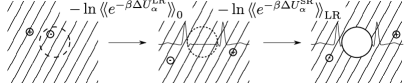
Figure 1: Division of the excess chemical potential into long-range polarization (left) and short-range chemical (right) steps. On the left, the solute and solvent are not interacting. In the center, the solute-solvent interaction energy is given by Eq. 11 and at the right the solvent and solute are fully interacting. This cycle was featured in Ref. 21.

The molecular picture of a uniform dipolar fluid above works well because local interactions were screened out by the replacement $1/r\to\operatorname{erf}(\eta r)/r$. Locally, the system behaves like a fluid with only short-range order while we focus on treating long-range correlations correctly. This leads us to the thermodynamic cycle of Fig. 1. Solvation of a charged species is divided into a long-range (LR) and a local (SR) contribution. The long-range step is performed first. According to the potential distribution theorem, the excess chemical potential of a solvated molecule, $\alpha$, is then expressed exactly as,

$$\beta\mu^{\text{ex}}_{\alpha} =-\ln\left\llangle e^{-\beta\Delta\hat{U}^{\text{LR}}_{\alpha}}\right\rrangle_{0}-\ln\left\llangle e^{-\beta\Delta\hat{U}^{\text{SR}}_{\alpha}}\right\rrangle_{\text{LR}}$$ (10)

$$\Delta\hat{U}^{\text{LR}}_{\alpha} \equiv\left<\hat{\rho}_{q}(r^{\prime})\vphantom{\frac{\operatorname{erf}(\eta_{\alpha}|r^{\prime}-r|)}{4\pi\epsilon_{0}|r^{\prime}-r|}\hat{\rho}_{\alpha}(r)}\right|\frac{\operatorname{erf}(\eta_{\alpha}|r^{\prime}-r|)}{4\pi\epsilon_{0}|r^{\prime}-r|}\left|\hat{\rho}_{\alpha}(r)\vphantom{\hat{\rho}_{q}(r^{\prime})\frac{\operatorname{erf}(\eta_{\alpha}|r^{\prime}-r|)}{4\pi\epsilon_{0}|r^{\prime}-r|}}\right>$$ (11)

$$\Delta\hat{U}^{\text{SR}}_{\alpha} \equiv\Delta\hat{U}_{\alpha}-\Delta\hat{U}^{\text{LR}}_{\alpha}.$$ (12)

The first term on the right of Eq. 10 is defined as $\beta\mu^{\text{ex,LR}}_{\alpha}$, the focus of this work. Here, $\hat{\rho}_{q}(r)$ is the instantaneous charge density at point $r$ corresponding to a single solvent microstate, while $\rho_{q}(r)$ is the average charge density which is zero by symmetry. Eq. 11 for the long-range interaction energy uses a bra-ket notation for the double-integral over $dr$ and $dr^{\prime}$. Hats are used used on quantities that depend on the molecular coordinates. Although this long-ranged interaction just contains the screened Coulomb energy, we note that it is simple to generalize $\eta_{\alpha}$ to $\eta_{\alpha}(r)$, so that different atoms can have different effective radii. The total solvation free energy, $\mu^{\text{ex}}_{\alpha}$, will not be affected by the choice of $\Delta\hat{U}_{\alpha}^{\text{LR}}$, but our results confirm that choosing $\sqrt{\pi}/2\eta=R_{B}$ minimizes the importance of the second, short-range step. The theory in Sec. III.2 is general enough to handle any choice for $\Delta\hat{U}^{\text{LR}}_{\alpha}$, including the full $\Delta\hat{U}_{\alpha}$ itself.

III.1 Correlation Functions

We have recently presented a simple Fourier-space method for inferring the direct correlation function from molecular dynamics data.Rogers (2018) This method of inverting the dipole correlation function to find an “effective dipole-dipole interaction energy” is synonymous with computing the direct correlation function of Ornstein-Zernike theory and the polarization structure factor of nonlocal response function theory.Matyushov (2004); Martin and Matyushov (2008) Formally, define a vector, $F_{\alpha}$, characterizing the orientation of a molecule of type $\alpha$. For example, the vector characterizing a molecule containing a point dipole could be $F=[1,p_{x},p_{y},p_{z}]^{T}$. Correlations between the density operators,

$$\hat{F}_{\alpha}(r)=\sum_{j=1}^{N_{\alpha}}F_{\alpha,j}\delta(r-r_{j}),$$ (13)

where $j$ indexes the $N_{\alpha}$ molecules of type $\alpha$, then report on both scalar and vector interactions.

Figure 2: Radial correlation functions ($h(r)=g(r)-1$) for water oxygen and dipole correlation functions. The top row (a-b) shows results from the SPC/E water model. The bottom row (c-d) shows results of the TIP5P water model. Water-dipole correlation functions (labeled wp) have units of $e_{0}$Å. The remaining lines in b and d are dipole-dipole correlations with radial ($\hat{r}\hat{r}^{T}$) or tangential symmetry ($I_{3}-\hat{r}\hat{r}^{T}$) and have units $(e_{0}\text{\AA{}})^{2}$.

The correlation function for these vectors is organized into a matrix where molecule indices are combined with vector indices and Fourier transformed,

$$Q_{\alpha\gamma}(k)\equiv\int_{V}e^{-ir\cdot k}\left\llangle\Delta\hat{F}_{\alpha}(r)\Delta\hat{F}_{\gamma}(0)^{T}\right\rrangle dr.$$ (14)

The integral ranges over the unit cell with volume $V$. To minimize error in the low-frequency components and to compute $Q$ efficiently, Eq. 14 is estimated from simulation data by averaging squared Fourier transforms ($\hat{\psi}_{\alpha}(k)\equiv\mathcal{F}[\hat{F}_{\alpha}(r)](k)$), so that $Q=\left\llangle\Delta\hat{\psi}\Delta\hat{\psi}^{\dagger}\right\rrangle/V$. Also, we define a potential after dividing by the volume so $\phi_{\alpha}(k)\equiv\mathcal{F}[\Phi_{\alpha}(r)](k)/V$. The Appendix gives helpful relations for the Fourier transform used here.

The correlation function is related to the Ornstein-Zernike definition,Beck et al. (2006a)

$$Q_{\alpha\gamma}(k)^{-1}=\frac{\partial{\beta\mu^{\text{id}}_{\alpha}}}{\partial{\rho_{\gamma}}}-c_{\alpha\gamma}(k).$$ (15)

Here,

$$\beta\mu^{\text{id}}_{\alpha}=\ln(\rho_{\alpha}\Lambda^{3}_{\alpha}/q^{\text{int}}_{\alpha})$$ (16)

is the ideal gas expression for the chemical potential of species $\alpha$.Beck et al. (2006b) Approximations to $Q$ are available both from analysis of experimental dataBopp et al. (1998), and from solutions to integral equations for charged or dipolar hard-sphere liquids.Wertheim (1971, 1984); Matyushov (2004) The results section presents the correlation functions and inverses computed from MD simulations of a series of 1:1 electrolyte solutions.

III.2 Solvation Potential Distribution

The basic quantity of the present theory is an exponential average,

$$Z[\Phi;V,\beta]=\left\llangle\exp{\left<\hat{\rho}\vphantom{\Phi}\right|\left.\Phi\vphantom{\hat{\rho}}\right>}\right\rrangle,$$ (17)

which is taken over the grand-canonical ensemble with $\mu$ describing the system before coupling to the solute (when $\Phi=0$). A constant shift of $\Phi$ has the same effect as changing the chemical potential in Eq. 17. The inner product in the exponent is defined in Appendix A and carries units of volume if both sides are in real space and inverse volume if both sides are in Fourier space. The long-range excess chemical potential can be written in terms of Eq. 17 as $\beta\mu^{\text{ex,LR}}_{\alpha}=-\ln Z[-\beta\Phi_{\alpha};n,V,\beta]$, which requires Legendre transformation of $\ln Z$ into the nVT ensemble, and defines $\Phi_{\alpha}$ to be the pair interaction field produced by the solute (by comparison to Eq. 11) as,

$$\Delta\hat{U}^{\text{LR}}_{\alpha}=\left<\Phi_{\alpha}\vphantom{\hat{\rho}}\right|\left.\hat{\rho}\vphantom{\Phi_{\alpha}}\right>=\left<\phi_{\alpha}\vphantom{\hat{\psi}}\right|\left.\hat{\psi}\vphantom{\phi_{\alpha}}\right>.$$ (18)

Figure 3: Inverse correlation functions in reciprocal space for water center of mass (left) and dipole correlation (right) functions. Note the units of the water-dipole correlation function contain an extra $1/e_{0}$Å. The top row (panels a,b) shows results from SPC/E and the bottom row (panels c,d) shows TIP5P results. See Eq. 26 for definitions. The value of $\eta$ plotted in panel b (SPC/E) is $1/1.8$Å and in panel d (TIP5P) is $1/1.6$Å.

Equation 17 is a moment generating function for the density field, $\hat{\rho}$, and we can define its corresponding density functional as the Legendre transform,

$$\mathcal{R}[\rho;V,\beta]\equiv\inf_{\Phi}\left[\ln Z[\Phi;V,\beta]-\left<\rho\vphantom{\Phi}\right|\left.\Phi\vphantom{\rho}\right>\right].$$ (19)

Eq. 19 is a generalized entropy, and is also called a (negative) rate function for the empirical distribution, $\left\llangle\hat{\rho}\right\rrangle_{V,\beta,\Lambda}$ in large deviation theory.Varadhan (2008); Touchette (2009) It is also the negative of the traditional “density functional.”Chandler et al. (1986) The functional $\mathcal{R}$ is maximized under extra constraints $\Lambda$ at constant volume and temperature when $\rho=\left\llangle\hat{\rho}\right\rrangle_{V,\beta,\Lambda}$. Stated in terms of Fourier-transformed densities and potentials, $\mathcal{R}$ satisfies

$$\frac{\partial{\mathcal{R}[\psi]}}{\partial{\psi^{\dagger}_{\alpha}(k)}} =-\phi_{\alpha}(k;\Lambda),$$

$$V\frac{\partial{\phi_{\alpha}(k;\Lambda)}}{\partial{\psi_{\gamma}(k^{\prime})}} =\delta_{k,k^{\prime}}Q^{-1}_{\alpha\gamma}(k;\Lambda).$$ (20)

The second equality requires translational invariance of the constrained ensemble ($V,T,\Lambda$) and explicitly acknowledges that the fluctuations in Eq. 14 depend on that ensemble.

Because $Z$ and $\mathcal{R}$ form a Legendre transform pair, $\beta\mu^{\text{ex,LR}}$ is simple to state in terms of $\mathcal{R}$,

$$-\beta\mu^{\text{ex,LR}}_{\alpha}=\sup_{\psi}\left[\mathcal{R}[\psi]-\left<\psi\vphantom{\beta\phi_{\alpha}}\right|\left.\beta\phi_{\alpha}\vphantom{\psi}\right>\right].$$ (21)

This equation may prove to be the most useful result in this paper. It shows that an approximation for Eq. 17 can be used to create a density functional that avoids the “charging” integration process of density-functional theory.Singer and Chandler (1985); Remsing and Weeks (2016) The maximization over densities in Eq. 21 can be carried out under fixed $n=\psi(0)$, but might also include other conditions. Those other constraints can be used to change the ensemble or even to fix the density to zero near the origin (as for the mean-spherical approximation). Because $\mathcal{R}$ was defined as a minimization problem, constraints on $\rho$ will be reflected physically by deviations of the pair potential, $\Phi$, which solves $\mathcal{R}$ away from the default ($\rho$-unconstrained) solution at $\Phi_{\alpha}$. Rigorously, constrained maximization is justified by the Gibbs conditioning principle, which states more formal conditions on the constraint and density spaces.Léonard and Najim (2002)

This development makes an important departure from traditional Ornstein-Zernike theory. Rather than seeking to provide an extra closure between direct and indirect correlation functions, our primary target is to model the rate function (Eq. 19). The Ornstein-Zernike relation is embedded in the structure of Eq. 20, so that the density fluctuations (radial distribution functions) come out as a consequence of a proper model for $\mathcal{R}$.

So far, the development from Eq. 10 through Eq. 21 has been formal and exact. To present analytical results in Sec. IV.2, we use the two-moment approximation,

$$\mathcal{R}[\psi]\simeq-\frac{1}{2}\left<\Delta\psi\vphantom{Q^{-1}\Delta\psi}\right|Q^{-1}\left|\Delta\psi\vphantom{\Delta\psi Q^{-1}}\right>,$$ (22)

where $\Delta\psi\equiv\psi-\psi_{0}$ and $\psi_{0}$ is the (Fourier) density of the uncoupled system. Technically, the domain of $\psi$ is limited to positive densities, which could also be included either as a better approximation to $\mathcal{R}[\psi]$ or as additional constraints. The results in this work do not include such a constraint.

Earlier work showed the utility of a Gaussian perturbation theory for the long-range part of the solvation free energy after forming a sufficiently large cavity.Rogers and Beck (2008, 2010); Friesen and V.Matyushov (2011); Remsing and Weeks (2016)

$$\mu^{\text{ex,LR}}_{\alpha}=\left\llangle\Delta\hat{U}^{\text{LR}}_{\alpha}\right\rrangle_{0}-\beta\sigma_{\text{LR}}^{2}/2+O(\beta^{2}).$$ (23)

Before forming a cavity, the first term in the expansion is zero by symmetry. We recover this result by inserting Eq. 22 into Eq. 21, adding $\phi(0)^{T}\psi(0)$ at $k=0$ to constrain the number of solvent molecules (with undetermined Lagrange multiplier $\phi(0)$), and maximizing. This leads to the identifications,

$$\Delta\psi(k) =-\beta Q(k)\phi_{\alpha}(k)+\delta_{k,0}Q(0)\phi(0),$$ (24)

and

$$-2\mu^{\text{ex,LR}}_{\alpha} =\beta\sigma_{\text{LR}}^{2}=\left<\delta_{k,0}\tfrac{\phi(0)}{\beta}-\phi_{\alpha}\vphantom{\Delta\psi}\right|\left.\Delta\psi\vphantom{\delta_{k,0}\tfrac{\phi(0)}{\beta}-\phi_{\alpha}}\right>$$

$$=\left<-\phi_{\alpha}\vphantom{\Delta\psi}\right|\left.\Delta\psi\vphantom{-\phi_{\alpha}}\right>$$ (25)

and shows that when Eq. 22 applies, the linear response approximation actually gives the ensemble average of the 1-particle density functions in the coupled state, and proves that the distribution of interaction energies, $\Delta\hat{U}^{\text{LR}}_{\alpha}$, is also Gaussian. The last simplification step in Eq. 25 happens because each component of the multiplier, $\phi_{j}(0)$, is chosen so that the corresponding molecule number does not change ($\Delta\psi_{j}(0)=\Delta n_{j}=0$).

For describing ionic solvation, specialize the solution components to a 1:1 electrolyte (e.g. NaCl) in water (modeled as a dipole so $F_{\text{H${}_{2}$O}}$ is a 3-component vector). Each density vector, $\psi(k)$, then has 5 components – cation and anion densities, $\psi_{q}$, plus water dipole vectors, $\psi_{p}$. In this basis, the screened interaction energy of an additional ion of charge $z_{\alpha}$ with solution (Eq. 11 and Eq. 18) has the form $\beta\phi_{\alpha}(k)=z_{\alpha}f(k)[1,-1,-ik]^{T}$ where $f(k)\equiv\beta e^{-k^{2}/4\eta^{2}}/k^{2}\epsilon_{0}$ is the Fourier-transform of the screened Coulomb operator (Eq. 2).

Figure 4: Electrolyte radial and dipole correlation functions overlayed for all five NaCl concentrations. Labels are as in Fig. 2. The right and left scales are identical even though the units differ. Peaks generally decrease toward zero with increasing concentration as can be inferred from comparison with corresponding plots in Ref. 61. The exception to this trend is the first minimum of the $\hat{r}\hat{r}^{T}$ component (d), which becomes more pronounced from 0.5 to 4M.

Equation 24 is the linear response of both water dipoles and ion densities to charged solutes. It is given, in the Gaussian approximation, by the convolution of the indirect correlation functions, $Q$, with the potential, $\phi_{\alpha}$. Since the potential is smooth and long-ranged, the small $k$ behavior of the correlation functions is the most important aspect of solvation. Second most is improving $\mathcal{R}$ beyond the Gaussian approximation to describe excluded volume effects.

IV Results

We show two key results. First, for sodium chloride solutions, the direct correlation functions exhibit error-function like screened forms with little dependence on ionic strength. Second, the long-range limits of these screened Coulomb forms motivate a random-phase like approximation whose analytical predictions for solution dielectric and ionic response re-derive the Born law and extend the Debye-Hückel theory with an ionic size-dependence that closely mirrors the full mean-spherical approximation result. Together, these results justify abandoning the Maxwell theory and its associated extensions of the Poisson equation. Instead, direct charge correlation functions, available from both experiment and simulations, form the basis for computable methods of solution response and solvation free energies.

IV.1 Simulation Correlation Functions

We simulated sodium chloride solutions in SPC/E using the Kirkwood-Buff forcefield model for ionsGee et al. (2011) replicating the simulation conditions in Ref. Weerasinghe and Smith (2003) but extending all simulations to at least 10 ns. Figures 2 and 3 show the water position and dipole indirect correlation functions ($F=[1,p_{x},p_{y},p_{z}]$) for pure SPC/EBerendsen et al. (1987) and TIP5PMahoney and Jorgensen (2000) water models under NVT conditions at 300 K. These were computed by inverse Fourier-transform of the correlations in reciprocal space. Deviations of $h(r)$ below the exact value of $-1$ near the origin indicate the amount of numerical error due to the band-limiting inherent in our method.

For all vector-scalar interactions plotted in real-space, the geometry should be pictured as with the vector fixed at the origin, pointing along the $+z$ axis. Positive interaction energies or low densities then describe unfavorable interactions of the dipole with molecules on the $+z$ hemisphere of radius $r$. Vector-vector interactions (e.g. between dipoles $p_{1}$ and $p_{2}$) along a separation direction $\hat{r}$ in real space are broken into parallel and isotropic components scaling with $p_{1}^{T}\hat{r}\hat{r}^{T}p_{2}$ or $p_{1}^{T}p_{2}$, respectively.

Figure 3 plots the components of water’s the inverse correlation function, $Q^{-1}(k)$. Panels b and d should be compared with Figs. 7 and  15 of Ref. 23, after noting that each point, $Q^{-1}(k)$, plotted here is the result of a $4\times 4$ matrix inverse. The two symmetry components of the dipole-dipole direct correlation function, $\chi\equiv Q^{-1}_{pp}$, in Fig. 3b and 3d are,

$$\chi(k)=\chi^{0}(|k|)\hat{k}\hat{k}^{T}+\chi^{1}(|k|)(I_{3}-\hat{k}\hat{k}^{T}).$$ (26)

Since the field produced by a dipole at the origin is proportional to $\hat{k}\hat{k}^{T}$, $\chi^{0}$ represents the effective energy governing the ‘longitudinal’ fluctuations of the second dipole in the direction parallel to the field lines created by the first water dipole, while $\chi^{1}$ represents ‘free’ or ‘tranverse’ fluctuations in the perpendicular direction. Without screening, these would be $\chi^{0}\epsilon_{0}/\beta=1+\epsilon_{0}/\rho_{w}\alpha$ and $\chi^{1}\epsilon_{0}/\beta=\epsilon_{0}/\rho_{w}\alpha$ in the lattice model. With screening, the $1$ in $\chi^{0}$ is replaced by the Fourier-transform of the screening charge distribution while $\chi^{1}$ is unchanged. This is the usual justification for using $\chi^{0}(0)=\chi^{1}(0)=V/\left\llangle M_{x}^{2}\right\rrangle$ (when $J=0$) to compute $\epsilon_{r}(0)=\beta/\chi(0)\epsilon_{0}+1$. However, away from $k=0$, only $\chi^{1}$ varies continuously. Fig. 3b and 3d clearly show that $\chi^{0}$ starts at 1, but decreases exponentially as $k$ increases. The fitted line uses $1/\eta=1.8$Å for SPC/E, which is equivalent to $R_{B}=1.6$Å. Interestingly, the $\chi^{1}$ component starts near 1/79, but increases to a larger constant value around $0.0540$ (SPC/E) or $0.0556$ (TIP5P). Using this in Eq. 9 gives only $19.5$ or $19.0$ for the dielectric, respectively. This behavior also appears in the MSA solution, and is more pronounced for dipolar-only solvents.Matyushov (2004)

Figure 5: Direct correlation functions for cation-water, anion-water, and water-water center to center interactions. Roughness of the water-water interaction is not physically meaningful, since it is within the water’s excluded volume.

Figures 4-9 show the ion-ion, ion-water, and water-water radial distribution functions and their transformations as a function of salt concentration. The direct interaction functions in real-space (Figs. 5, 6, 8, and 9) follow screened Coulomb electrostatic laws so closely that we have subtracted out the screened forms and plotted the differences instead. Subtracted parts are shown so that the two curves can be visually added to get the total $Q^{-1}$. Ion-water (Figs. 5 and 6) and ion-ion interactions (Fig. 8) show negligible concentration dependence.

Figure 6: Ion-dipole direct correlation functions for 1M and 4M salt concentrations, scaled by the Coulomb constant, $\xi=1/4\pi\epsilon_{0}$. The long-range Coulomb expression given by the dashed-dotted line at the bottom was subtracted from each of the lines using $\eta_{+p}=1/1.9$Å and $\eta_{-p}=1/2.3$Å. The only major feature that remains is a peak around the distance of the first maximum in $g(r)$ (Fig. 4).

Figure 7 shows the ion-ion interactions in reciprocal space to have the expected, ideal, $1/\rho$ contribution and the $k^{-2}$ divergence near the origin.Attard (1993) The $k\to 0$ limit in Fig. 7a and 7b can be used to find the Kirkwood-Buff coefficients for single-ions.Weerasinghe and Smith (2003); Schnell et al. (2013); Rogers (2018) A log-log plot (Fig. 7c,d) shows the $k^{-2}$ divergence transitions to an exponential-like screening around $k=1$Å^-1 before flattening out due to the ideal ($1/\rho$) contribution. These profiles were used to identify appropriate screening lengths for each ion, resulting in $1/\eta_{++}=2.2$Å and $1/\eta_{--}=2.65$Å. Note that Born radii are expected to be temperature and pressure-dependent. However, our results indicate that they are not sensitive to salt concentration in the 0-4M range.

Figure 7: Electrolyte direct correlation functions in reciprocal space for varying salt concentration. Panels a and b show the average interaction of anions and cations with all other ions: $(Q^{-1}_{++}+Q^{-1}_{+-})/2-1/2\beta\rho$ and $(Q^{-1}_{--}+Q^{-1}_{+-})/2-1/(2\beta 4\text{M})$, respectively. Panels c and d show $Q^{-1}_{++}$ and $Q^{-1}_{--}$ (resp.) on a log-log scale near the origin. The light gray line is $e^{-k^{2}/4\eta^{2}}/\epsilon_{0}k^{2}+1/2\beta\rho$ (cf. Eq. 27) and fits to $1/\eta_{++}=2.2$Å and $1/\eta_{--}=2.65$Å.

The ion center of mass direct correlation functions in Fig. 8 are surprisingly featureless apart from the $1/r$ interaction. An unexplainable, small linear trend shows up in Fig. 8b at long range with a positive slope for like-charged ion interaction and a negative slope for cation-anion interactions. At short-range, the like-charged interaction shows numerical noise before a steep, repulsive increase. This does not appear in the cation-anion interaction. This short-range behavior is not directly linked to interaction energies. In the mean-spherical approximation, it is treated as a fitting parameter to achieve excluded volume in $g(r)$.

Figure 8: Ion center of mass direct correlation functions scaled by the Coulomb constant, $\xi=1/4\pi\epsilon_{0}$. Panel a shows concentration dependence of cation-anion interactions (using $\eta=1/2.7$Å), while panel b compares direct correlation functions between like and unlike ions. In every case, the curves are drawn after subtracting the screened Coulomb expression appropriate for each pair (dashed-dotted lines). The screening distances used for like ions were the same as in Fig. 7.

Figure 9: Water-water direct correlation functions. Panel a shows center to center interactions, b shows center to dipole interactions (positive if the water dipole faces the separation distance), and panels c and d show co-linear and perpendicular components of the dipole-dipole interaction. The last two curves are drawn after subtracting the appropriate long-range Coulomb expression (indicated by the labeled dash-dotted line).

Fig. 9 returns our focus to the number and dipole density response behavior of water. The dipole-dipole interaction energies for co-linear aligned and in-plane parallel orientations (Fig. 9c,d, respectively) both follow the expected trends. Within this dipolar response function description, local effects only appear within the first 6Å. Interesting salt-concentration effects show up in the the shape of the water solvation shell around a water fixed at the origin (Fig. 9b). This may be linked to electrostriction and specific-ion effects.Mazzini and Craig (2017)

IV.2 Approximate long-range limiting laws

We show the utility of the theory above by deriving simple analytical expressions for long-range ionic chemical potentials (Eq. 23) using a “screened MSA” (for a 1:1 electrolyte with equal cation and anion concentrations, $\rho$),

$$Q^{-1}(k)=\begin{bmatrix}\rho^{-1}+f&-f&ik^{T}f\\ -f&\rho^{-1}+f&-ik^{T}f\\ -ikf&ikf&\chi\end{bmatrix},$$ (27)

where $\chi=I_{3}\beta/\rho_{w}\alpha+fkk^{T}$ is the lattice result, containing contributions from water polarizability and the screened dipole-dipole interaction energy. To properly express the energy contribution from polarizing the surface, the dipole-dipole energy at $k=0$, should be replaced by the depolarization tensor ($\chi(0)=I_{3}\beta/\rho_{w}\alpha+\beta J$).Ballenegger (2014) Eq. 27 is essentially a mean-spherical approximation, and is a caricature of the low-$k$ behavior found in Sec. IV.1 with only one $\eta$ value.

This ansatz is simple, supported by our simulation results and yields both the Born theory and a mean-spherical approximation-like Debye-Hückle theory as limits. However, it is not intended to be used in practice, since Ref. 23 contains analytical expressions for $Q$ that match our simulation results for water much more closely.

IV.3 Born Limit

The developments above make re-derivation of Eq. 8 a simple matter of removing charge-ion interactions. To accomplish this, delete the top two rows and columns from $Q^{-1}$ in Eq. 27 and in Eq. 25. The result is,

$$\beta^{2}\sigma^{2}_{\text{LR,Born}} =z_{\alpha}^{2}\left<k\vphantom{f^{2}(k)\chi^{-1}k}\right|f^{2}(k)\chi^{-1}\left|k\vphantom{kf^{2}(k)\chi^{-1}}\right>$$

$$=\frac{z_{\alpha}^{2}}{V}\sum_{k}f(k)-\bar{f}(k),$$ (28)

which introduces a definition for the scaled interaction energy,

$$\bar{f}(k)\equiv f/(1+e^{-k^{2}/4\eta^{2}}\alpha\rho_{w}/\epsilon_{0})\equiv f/\epsilon_{r}(k).$$ (29)

The last equality also defines the “dielectric function,” $\epsilon_{r}$, of the lattice model. It reduces to Eq. 9 when $\eta\to\infty$. The $k^{-2}$ divergence at $k=0$ integrates to a contribution that scales as $1/V$.

Because the solvent density response is purely along the longitudinal ($\hat{k}$) direction, it can be written in two forms,

$$\Delta\psi_{p}=iz_{\alpha}f\chi^{-1}k=\frac{iz_{\alpha}k}{k^{2}}\left(1-1/\epsilon_{r}\right).$$ (30)

It is extremely important to notice the difference between $1/\epsilon_{r}(k)$, defined for mathematical convenience in Eq. 29, and the indirect dipole-dipole correlation function, $\chi^{-1}$, which gives the both transverse and longitudinal contributions to the orientation response. Both these correlations are long-ranged, while their inverses appear short-ranged. However, $\epsilon_{r}$ is only short-ranged in real-space when there are no other interactions besides electrostatic ones (hence the $k^{-1}$ prefactor), while $\chi(r)$ is not short-ranged until the electrostatic $1/r^{3}$ term is subtracted.

IV.4 Debye-Hückel Limit

Maximizing only the dipoles, $\Delta\psi_{p}$, in Eq. 22 leads to the linear response equation,

$$Q^{-1}_{pp}|\Delta\psi_{p}\rangle+Q^{-1}_{pq}|\Delta\psi_{q}\rangle+|\beta\phi_{p}\rangle=0,$$ (31)

with obvious notation for 2- and 3-component sub-blocks of Eq. 27. Replacing this back in Eq. 22 and simplifying leads to a charge-only system with $Q^{-1}_{qq}$ scaled by the effective dielectric (Eq. 29),

$${\bar{Q}}^{-1}_{qq}(k) =\begin{bmatrix}\rho^{-1}+\bar{f}&-\bar{f}\\ -\bar{f}&\rho^{-1}+\bar{f}\\ \end{bmatrix},$$ (32)

$$\text{and }\beta\bar{\phi}_{q} =[\bar{f},-\bar{f}]^{T}.$$ (33)

Inverting Eq. 32 yields the ionic charge density induced by an external potential from a charge at the origin,

$$\Delta\psi_{q}(k)=-z_{\alpha}\left(\frac{\rho\bar{f}}{1+2\rho\bar{f}}-\delta_{k}\right)\begin{bmatrix}1\\ -1\end{bmatrix}.$$ (34)

Ref. 68 also found Eq. 34 by applying the random phase approximation to a fluid of screened, soft-core ions. They obtain a closed form for its Fourier transform ($h(r)$) and show that it predicts a cross-over from exponential to damped oscillatory behavior at high ionic strength.

Collecting all the terms in Eq. 22 created by our procedure, the fluctuations in the solvation potential of an ion with charge $z_{\alpha}$ is given by the sum,

$$\sigma^{2}_{\text{LR}} =\sigma^{2}_{\text{LR,Born}}+\sigma^{2}_{\text{LR,DH}}$$ (35)

$$\beta^{2}\sigma^{2}_{\text{LR,DH}} =\frac{z_{\alpha}^{2}}{V}\sum_{k\neq 0}\frac{2\rho\bar{f}^{2}(k)}{1+2\rho\bar{f}}.$$ (36)

Using the relations for the inner product developed in Appendix A, the summation in Eq. 36 goes over to the inverse Fourier transform as the cell volume increases,

$$\beta^{2}\sigma^{2}_{\text{LR,DH}} \to\frac{\beta z_{\alpha}^{2}}{(2\pi)^{3}\epsilon_{r}\epsilon_{0}}\int_{0^{+}}^{\infty}\frac{4\pi\kappa^{2}e^{-k^{2}/2\eta^{2}}}{k^{2}+\kappa^{2}e^{-k^{2}/4\eta^{2}}}\;dk$$

$$=\frac{\beta z_{\alpha}^{2}\kappa}{4\pi^{2}\epsilon_{r}\epsilon_{0}}\int_{-\infty}^{\infty}\frac{e^{-k^{2}u^{2}}}{k^{2}e^{k^{2}u^{2}}+1}\;dk.$$ (37)

Here $\kappa^{2}\equiv 2\beta\rho/\epsilon_{r}\epsilon_{0}$ and $u^{2}\equiv\kappa^{2}/4\eta^{2}=\kappa^{2}R_{\text{B}}^{2}/\pi$. When $u$ goes to zero (zero ion radius), the integral becomes $\pi$, and we recover the classical Debye-Hückel result for the solvation free energy using Eq. 37 with Eq. 23.

For finite $\eta$, $\epsilon_{r}$ is $k$-dependent, and the integral is strictly smaller than $\pi$. It decreases with increasing $\kappa R$ – making ionic solvation less favorable. We calculated the integral numerically and verified that it compares well with the mean spherical approximation result for the electrostatic free energy component with ion radius $R_{B}$.Blum (1975)

V Discussion

The assumption in Eq. 27 used to derive Born and modified DH laws is essentially the random phase approximation (RPA) of fluid density functional theory. A similar derivation has recently been presented (starting from the RPA) by Frydel and Ma.Frydel and Ma (2016) They do not include screening and thus arrive at the linearized Poisson-Boltzmann equation. Earlier work showed the utility of this approximation for describing charge reversal near a charged surface.Frydel and Levin (2013) In later work, they caution that the RPA, being equivalent to a variational Gaussian approximation, has the same weaknesses as a mean-field approximation and loses applicability at strong coupling.Xiang and Frydel (2017) The primary difference in this work is that we do not use the adiabatic connection to charge up the whole system at once, but only calculate the effect of adding a single ion in a self-consistent way. This frees approximations like Eq. 22 from having to represent the density of the entire system. The RPA works well because the solute potential, $\Phi_{\alpha}$, is concentrated at long range, near $k=0$.

We view the focus on addition of a single molecule to a pre-existing fluid as the major reason for success of the present theory. An entire fluid constructed from soft ions has very different properties. It has been investigated as the “ultrasoft restricted primitive model” (URPM) of penetrable electrolytes such as charged polymers.Nikoubashman et al. (2012) The screening prevents Coulomb collapse in the URPM, but allowing ion overlap removes the competition between long-range attraction and short-range excluded volume underpinning most density functional closures, explaining their difficulty in predicting its phase diagram.

It is hard to compare our simulation results with the body of literature on the Hubbard-Stratonovich transformation, which is a Fourier instead of a Legendre transform. The major difficulty is technical. Since the transformation introduces an imaginary, auxiliary field with an infinite number of degrees of freedom, most of its expressions are related to distributions of the imaginary potential and cannot be easily compared to molecular simulations. Analytically, the theory is commonly used in combination with a mean-field type expression for the potential or density functional which can result in various modified Poisson-Boltzmann theories depending on this approximation.Buyukdagli and Ala-Nissila (2013); Levy et al. (2013); Pujos and Maggs (2015) When employing the variational Gaussian approximation within the statistical field theory, the results of Sec. IV.2 appear almost exactly with the same conclusions.Wang (2010); Martin et al. (2016) Nevertheless, the picture there is of the URPM model and is more difficult to extend to non-pairwise interactions. In addition, entropic terms similar to the primitive available volume approximation ($-\ln(1-V_{0}\rho)$) have been successfully used to account for the free energy of cavity formation in related works.Borukhov et al. (1997); Koehl et al. (2009)

The physical picture of solvent response gained from Fig. 9 is that the “local electric field,” which determines the force felt by a solvent dipole has special contributions from the first two or three solvation layers. Beyond that, it has the expected form of an integral over dipole-dipole electrostatic $1/r^{3}$ terms. Two maxima surround a sharp minimum in $\chi^{0}$ near the first peak of the water-water radial distribution (Fig. 9c) – so that the dipole-dipole interaction is slightly more repulsive for waters deviating from the optimal distance. This behavior likely reflects quadrupolar forces causing correlations between the position and orientation angle of first-shell waters. The isotropic part of the local electric field (that scales with the cosine of the water-water angle, $\mu\cdot\mu$) in Fig. 9d mainly follows a typical screened form, but shows an extra tendency for waters closer than 3Å to take antiparallel orientations.Martin and Matyushov (2008)

For ion-water association, Fig. 6 shows a single peak where the usual ion-dipole interaction is strengthened, while Fig. 5 shows a local minimum for the center-to-center interaction. This strengthening occurs for both ions and both interactions right at the maximum of the ion-water radial distribution function. The extra dipolar response is direct evidence for the hypothesis that the first solvent dipole layer at the solute/solvent interface should be scaled from the Maxwell theory.Heyden et al. (2012) The extra center-to-center interaction provides an energetic basis for electrostriction. Both are associated with specific-ion effects.Wachter et al. (2005); Beck (2011)

VI Conclusion

The limiting cases studied throughout Sec. IV.2 establish the utility of this theory, and serve as a guide for translating the language of dielectric polarization into structural, energetic terms. Future work should explore the key features of the correlation functions responsible for experimental evidence of specific ion effects.

We have taken one step, showing the direct correlation function found from simulations has a surprisingly good agreement with the random phase and mean spherical approximations. They are indistinguishable past the second solvation shell of water. Even within the first and second solvation shells, the effective energy only oscillates about the error-function screened form. One way to rationalize the far-field result is to note that long-range electrostatic ordering (and charge density fluctuations) does not depend sensitively on local charge ordering. Rigorously, higher-order multipoles have a rapidly decreasing interaction radius.

We reiterate here the importance of distinguishing between the ideal dielectric continuum theory, for which $\epsilon_{r}$ can be usefully defined, and real solutions containing additional local interactions besides electrostatics. As Eq. 5 and 30 illustrate, the inverse correlation function is more informative than an inferred dielectric function.

This observation helps give a simple mathematical structure to a nonlocal response theory for solution density response to the solute’s molecular field. It is well-known that a majority of the solvation free energy in polar liquids is due to long-range solvent electrostatic response. Most dielectric theories spend a lot of effort finding a solute-solvent boundary that makes bulk dielectric polarization theories give accurate free energies. The density response paradigm parallels density functional theories by focusing on reproducing average solvent dipole (and ionic) densities conditional on interaction with the solute. Eq. 21 then provides the excess chemical potential exactly. Using a screened electrostatic interaction removes non-physical issues with singularities of the Coulomb potential at the origin, while capturing long-range contributions.

The same division into short and perturbative long-range interactions is a crucial step in local molecular field (LMF) theory,Chen and Weeks (2006); Rodgers and Weeks (2008); Remsing and Weeks (2016). While LMF theory takes an additional step to find a long-range Coulomb field self-consistently, the present work has the more modest goal of describing only single-solute energetics. Our connection with solution spatial response functions allows for detailed tests of the theory, and suggests simple generalizations to self-consistent spatial and time-dependent problems, for which response data are already available.Bagchi and Chandra (1989); Salacuse and Egelstaff (2001)

The technical foundation for the theory applied the Gibbs conditioning principle to transform the grand potential into an exact expression for the solvation free energy.Léonard and Najim (2002) This appears to be a novel route for eliminating the Hubbard-Stratonovich transform that proceeds directly to a computable density functional, and for expressing the free energy in conventional density functional theories.Kovalenko and Hirata (2000) Although few density functionals treat molecular orientation in an angular expansion,Rogers (2015) many ideas from both integral equations and density functional theory can still be carried over into the present formalism. Another obvious addition is to include the contribution of energetic degeneracy of solvent dipole orientations belonging to a given dipole density in Eq. 22. This would begin to address the dispersion contribution identified for the lattice model in Eq. 7.

There are many important questions which might be addressed with this theory. We have not attempted to calculate the second step in Fig. 1, which involves forming a cavity at the center of a screened field. It has, however, been explicitly computed by othersRemsing and Weeks (2016) who have shown that cavity formation in water creates a positive relative potential at the center.Ashbaugh and Pratt (2006); Rogers and Beck (2010); Molavi Tabrizi et al. (2017); Duignan et al. (2017) That asymmetry lowers the free energy of anionic solvation and, by path equivalence, makes cavity formation in step 2 of Fig. 1 easier after polarizing water with a negative potential. Including both polarization and cavity formation in the first step (by adding an occupancy constraint)Hummer et al. (1996) provides a possible route to combining and comparing these ideas. The limit, $Q^{-1}(0)$, provides $\partial\beta\mu/\partial\rho$ via the Kirkwood-Buff theory,Rogers (2018) and, given a predictive theory for $Q$, gives a more traditional route to solvation free energies.Perry et al. (1988); Weerasinghe and Smith (2003); Schnell et al. (2013) Further, cluster expansion of Eq. 17 could be used to include explicit solvent molecules near the solute as a means to systematically improve approximations to Eq. 21 in a quasi-chemical way.Beck et al. (2006a); Pratt and Ashbaugh (2003); Rogers et al. (2012)

Appendix A Inner Product Definition

The definition of the inner product in Eq. 11 is straightforward, but extremely useful both for simplifying our notation and performing computations. Denote a vector of $\nu$ functions each in $\mathbb{R}^{3}\to\mathbb{C}^{d}$, as $f$ and another vector as $g$. The inner product is the sum-integral,

$$\left<f\vphantom{g}\right|\left.g\vphantom{f}\right>=\sum_{\alpha=1}^{\nu}\int_{V}f_{\alpha}(r)^{\dagger}g_{\alpha}(r)\;dr,$$ (38)

where the integration ranges over the 3D unit cell with volume, $V$. The dagger denotes the complex-transpose and is used so that $f_{\alpha}(r)^{\dagger}g_{\alpha}(r)$ is a scalar. Note that $\left<f\vphantom{g}\right|\left.g\vphantom{f}\right>$ is the complex conjugate of $\left<g\vphantom{f}\right|\left.f\vphantom{g}\right>$, motivating our adoption of Dirac brackets.

Defining Fourier transforms of each function as,

$$\mathcal{F}[f_{\alpha}](k)\equiv\int_{V}e^{-ik\cdot r}f_{\alpha}(r)\;dr,$$ (39)

the Fourier-Plancherel theorem proves the equivalence of the inner product with the infinite sum,

$$\left<f\vphantom{g}\right|\left.g\vphantom{f}\right>=\frac{1}{V}\sum_{\alpha=1}^{\nu}\sum_{k}\mathcal{F}[f_{\alpha}](k)^{\dagger}\mathcal{F}[g_{\alpha}](k).$$ (40)

In Eq. 40, the summation is over the reciprocal lattice, $k\in\{2\pi L^{-1}z|z\in\mathbb{Z}^{3}\}$, where $L$ is a $3\times 3$ matrix whose rows are unit cell translation vectors. In the text we use the same inner product symbol for both representations, so $\left<\mathcal{F}[f]\vphantom{\mathcal{F}[g]}\right|\left.\mathcal{F}[g]\vphantom{\mathcal{F}[f]}\right>\equiv\left<f\vphantom{g}\right|\left.g\vphantom{f}\right>$.

In the limit of infinite volume, the reciprocal lattice sum goes over to,

$$\lim_{V\to\infty}\frac{1}{V}\sum_{k}r(k)=\int_{\mathbb{R}^{3}}\frac{r(k)\;dk}{(2\pi)^{3}}.$$ (41)

This work uses hats (as in $\Delta\hat{U}_{\alpha}$) to denote functions which depend on the system microstate. This is distinct from their usual quantum-mechanical interpretation as operators. Mathematically, the hat just denotes a random variable here.

Operator notation is defined similarly to the inner-product notation,

$$\left<f\vphantom{Mg}\right|M\left|g\vphantom{fM}\right> =\sum_{\alpha\gamma}\int_{V}\int_{V}f_{\alpha}(r)M_{\alpha\gamma}(r-r^{\prime})g_{\gamma}(r^{\prime})drdr^{\prime}$$ (42)

$$=\frac{1}{V}\sum_{\alpha\gamma}\sum_{k}\mathcal{F}[f_{\alpha}](k)^{\dagger}\mathcal{F}[M_{\alpha\gamma}](k)\mathcal{F}[g_{\gamma}](k).$$ (43)

References

- Ren et al. (2012) P. Ren, J. Chun, D. G. Thomas, M. J. Schnieders, M. Marucho, J. Zhang, and N. A. Baker, Quart. Rev. Biophys. 45, 427 (2012).
- Mennucci et al. (1997) B. Mennucci, E. Cancès, and J. Tomasi, J. Phys. Chem. B 101, 10506 (1997).
- Schnieders and Ponder (2007) M. J. Schnieders and J. W. Ponder, J. Chem. Theory Comput. 3, 2083 (2007).
- Duignan et al. (2013) T. T. Duignan, D. F. Parsons, and B. W. Ninham, J. Phys. Chem. B 117, 9412 (2013).
- Buchner and Barthel (2001) R. Buchner and J. Barthel, Annu. Rep. Prog. Chem. C 97, 349 (2001).
- Skaf and Ladanyi (1995) M. S. Skaf and B. M. Ladanyi, J. Chem. Phys. 102, 6542 (1995).
- Omelyan (1997) I. P. Omelyan, Physica A 247, 121 (1997).
- Bopp et al. (1996) P. A. Bopp, A. A. Kornyshev, and G. Sutmann, Phys. Rev. Lett. 76, 1280 (1996).
- Bopp et al. (1998) P. A. Bopp, A. A. Kornyshev, and G. Sutmann, J. Chem. Phys. 109, 1939 (1998).
- Stern and Feller (2003) H. A. Stern and S. E. Feller, J. Chem. Phys. 118, 3401 (2003).
- Ballenegger and Hansen (2005) V. Ballenegger and J.-P. Hansen, J. Chem. Phys. 122, 114711 (2005).
- Zasetsky and Svishchev (2001) A. Y. Zasetsky and I. M. Svishchev, J. Chem. Phys. 115, 1448 (2001).
- Friesen and V.Matyushov (2011) A. D. Friesen and D. V.Matyushov, Chem. Phys. Lett. 511, 256 (2011).
- Schaaf and Gekle (2015) C. Schaaf and S. Gekle, Phys. Rev. E 92, 032718 (2015).
- Schaaf and Gekle (2016) C. Schaaf and S. Gekle, J. Chem. Phys. 145, 084901 (2016).
- Matyushov (2014) D. V. Matyushov, J. Chem. Phys. 140, 224506 (2014).
- Bagchi (2001) B. Bagchi, Chem. Rev. 105, 3197 (2001).
- Martin et al. (2014) D. R. Martin, D. Fioretto, and D. V. Matyushov, J. Chem. Phys. 140, 035101 (2014).
- Martin and Matyushov (2017) D. R. Martin and D. V. Matyushov, J. Chem. Phys. 147, 084502 (2017).
- Heyden et al. (2012) M. Heyden, D. J. Tobias, and D. V. Matyushov, J. Chem. Phys. 137, 235103 (2012), 10.1063/1.4772000.
- Remsing and Weeks (2016) R. C. Remsing and J. D. Weeks, J. Phys. Chem. B 120, 6238 (2016).
- Beglov and Roux (1997) D. Beglov and B. Roux, J. Phys. Chem. B 101, 7821 (1997).
- Matyushov (2004) D. V. Matyushov, J. Chem. Phys. 120, 7532 (2004).
- Martin and Matyushov (2008) D. R. Martin and D. V. Matyushov, J. Chem. Phys. 129, 174508 (2008).
- Perry et al. (1988) R. L. Perry, J. D. Massie, and P. T. Cummings, Fluid Phase Equil. 39, 227 (1988).
- Kovalenko and Hirata (2000) A. Kovalenko and F. Hirata, J. Chem. Phys. 112, 10391 (2000).
- Maribo-Mogensen et al. (2012) B. Maribo-Mogensen, G. M. Kontogeorgis, and K. Thomsen, Ind. Eng. Chem. Res. 51, 5353 (2012).
- Raineri and Stell (2001) F. O. Raineri and G. Stell, J. Phys. Chem. B 105, 11880 (2001).
- Dyer et al. (2008) K. M. Dyer, J. S. Perkyns, G. Stell, and B. M. Pettitt, J. Chem. Phys. 129, 104512 (2008).
- Overduin and Patey (2012) S. D. Overduin and G. N. Patey, J. Phys. Chem. B 116, 12014 (2012).
- Zhao et al. (2013) S. Zhao, Y. Liu, H. Liu, and J. Wu, J. Chem. Phys. 139, 064509 (2013).
- Chuev et al. (2014) G. N. Chuev, I. Vyalov, and N. Georgi, J. Comput. Chem. 35, 1010 (2014).
- Sheng and Wu (2016) S. Sheng and J. Wu, Mol. Phys. 114, 2351 (2016).
- Sergey V. Novikov (1995) A. V. V. Sergey V. Novikov, J. Phys. Chem. 99, 14573 (1995).
- Ravichandran and Bagchi (1996) S. Ravichandran and B. Bagchi, Phys. Rev. E 54, 3693 (1996).
- Papazyan and Warshel (1997) A. Papazyan and A. Warshel, J. Phys. Chem. B 101, 11254 (1997).
- Essmann et al. (1995) U. Essmann, L. Perera, M. L. Berkowitz, T. Darden, H. Lee, and L. G. Pedersen, J. Chem. Phys. 103, 8577 (1995).
- Toukmaji et al. (2000) A. Toukmaji, C. Sagui, J. Board, and T. Darden, J. Chem. Phys. 113, 10913 (2000).
- Zhou et al. (1992) H.-X. Zhou, B. Bagchi, A. Papazyan, and M. Maroncelli, J. Chem. Phys. 97, 9311 (1992).
- Ballenegger (2014) V. Ballenegger, J. Chem. Phys. 140, 161102 (2014).
- Johnson (2011) S. G. Johnson, in Casimir Physics, Lecture Notes in Physics, Vol. 834 (Springer, 2011) Chap. 6, pp. 175–218.
- Dyson (1972) F. J. Dyson, Bull. Amer. Math. Soc. 78, 635 (1972).
- Diehl et al. (1997) A. Diehl, M. C. Barbosa, and Y. Levin, Phys. Rev. E 56, 619 (1997).
- Martin et al. (2016) J. M. Martin, W. Li, K. T. Delaney, and G. H. Fredrickson, J. Chem. Phys. 145, 154104 (2016).
- Wang (2010) Z.-G. Wang, Phys. Rev. E 81, 021501 (2010).
- Pujos and Maggs (2015) J. S. Pujos and A. C. Maggs, J. Chem. Theory Comput. 11, 1419 (2015).
- Frydel and Ma (2016) D. Frydel and M. Ma, Phys. Rev. E 93, 062112 (2016).
- Xiang and Frydel (2017) Y. Xiang and D. Frydel, J. Chem. Phys. 146, 194901 (2017).
- Rogers (2018) D. M. Rogers, “Extension of Kirkwood-Buff theory to the canonical ensemble,” (2018), submitted.
- Beck et al. (2006a) T. L. Beck, M. E. Paulaitis, and L. R. Pratt, “Statistical tentacles,” in The Potential Distribution Theorem and Models of Molecular Solutions (Cambridge, New York, 2006) Chap. 6, pp. 123–141.
- Beck et al. (2006b) T. L. Beck, M. E. Paulaitis, and L. R. Pratt, “Statistical thermodynamic necessities,” in The Potential Distribution Theorem and Models of Molecular Solutions (Cambridge, New York, 2006) Chap. 2, pp. 23–31.
- Wertheim (1971) M. S. Wertheim, J. Chem. Phys. 55, 4291 (1971).
- Wertheim (1984) M. S. Wertheim, J. Stat. Phys. 35, 19 (1984).
- Varadhan (2008) S. R. S. Varadhan, Ann. Prob. 36, 397 (2008).
- Touchette (2009) H. Touchette, Phys. Rep. 478, 1 (2009).
- Chandler et al. (1986) D. Chandler, J. D. McCoy, and S. J. Singer, J. Chem. Phys. 85, 5971 (1986).
- Singer and Chandler (1985) S. J. Singer and D. Chandler, Molecular Physics 55, 621 (1985).
- Léonard and Najim (2002) C. Léonard and J. Najim, Bernoulli 8, 721 (2002).
- Rogers and Beck (2008) D. M. Rogers and T. L. Beck, J. Chem. Phys. 129, 134505 (2008).
- Rogers and Beck (2010) D. M. Rogers and T. L. Beck, J. Chem. Phys. 132, 014505 (2010).
- Weerasinghe and Smith (2003) S. Weerasinghe and P. E. Smith, J. Chem. Phys. 119, 11342 (2003).
- Gee et al. (2011) M. B. Gee, N. R. Cox, Y. Jiao, N. Bentenitis, S. Weeerasinghe, and P. E. Smith, J. Chem. Theory Comput. 7, 1369 (2011).
- Berendsen et al. (1987) H. J. C. Berendsen, J. R. Grigera, and T. P. Straatsma, J. Phys. Chem. 91, 6269 (1987).
- Mahoney and Jorgensen (2000) M. W. Mahoney and W. L. Jorgensen, J. Chem. Phys. 112, 8910 (2000).
- Attard (1993) P. Attard, Phys. Rev. E 48, 3604 (1993).
- Schnell et al. (2013) S. K. Schnell, P. Englebienne, J.-M. Simon, P. Krüger, S. P. Balaji, S. Kjelstrup, D. Bedeaux, A. Bardow, and T. J. Vlugt, Chem. Phys. Lett. 582, 154 (2013).
- Mazzini and Craig (2017) V. Mazzini and V. S. J. Craig, Chem. Sci. 8, 7052 (2017).
- Nikoubashman et al. (2012) A. Nikoubashman, J.-P. Hansen, and G. Kahl, J. Chem. Phys. 137, 094905 (2012).
- Blum (1975) L. Blum, Mol. Phys. 30 (1975).
- Frydel and Levin (2013) D. Frydel and Y. Levin, J. Chem. Phys. 138, 174901 (2013).
- Buyukdagli and Ala-Nissila (2013) S. Buyukdagli and T. Ala-Nissila, Phys. Rev. E 87, 063201 (2013).
- Levy et al. (2013) A. Levy, D. Andelman, and H. Orland, J. Chem. Phys. 139, 164909 (2013).
- Borukhov et al. (1997) I. Borukhov, D. Andelman, and H. Orland, Phys. Rev. Lett. 79, 435 (1997).
- Koehl et al. (2009) P. Koehl, H. Orland, and M. Delarue, J. Phys. Chem. B 113, 5694 (2009).
- Wachter et al. (2005) W. Wachter, W. Kunz, R. Buchner, and G. Hefter, J. Phys. Chem. A 109, 8675 (2005).
- Beck (2011) T. L. Beck, J. Phys. Chem. B 115, 9776 (2011).
- Chen and Weeks (2006) Y.-G. Chen and J. D. Weeks, Proc. Nat. Acad. Sci. USA 103, 7560 (2006).
- Rodgers and Weeks (2008) J. M. Rodgers and J. D. Weeks, Proc. Nat. Acad. Sci. USA 105, 19136 (2008).
- Bagchi and Chandra (1989) B. Bagchi and A. Chandra, J. Chem. Phys. 90, 7338 (1989).
- Salacuse and Egelstaff (2001) J. J. Salacuse and P. A. Egelstaff, Phys. Rev. E 64, 051201 (2001).
- Rogers (2015) D. M. Rogers, J. Chem. Phys. 142, 074101 (2015).
- Ashbaugh and Pratt (2006) H. S. Ashbaugh and L. R. Pratt, Rev. Mod. Phys. 78, 159 (2006).
- Molavi Tabrizi et al. (2017) A. Molavi Tabrizi, S. Goossens, A. Mehdizadeh Rahimi, C. D. Cooper, M. G. Knepley, and J. P. Bardhan, J. Chem. Theory Comput. 13, 2897 (2017), pMID: 28379697, http://dx.doi.org/10.1021/acs.jctc.6b00832 .
- Duignan et al. (2017) T. T. Duignan, M. D. Baer, G. K. Schenter, and C. J. Mundy, J. Chem. Phys. 147, 161716 (2017).
- Hummer et al. (1996) G. Hummer, S. Garde, A. E. García, A. Pohorille, and L. R. Pratt, Proc. Nat. Acad. Sci. USA 93, 8951 (1996), http://www.pnas.org/content/93/17/8951.full.pdf+html .
- Pratt and Ashbaugh (2003) L. R. Pratt and H. S. Ashbaugh, Phys. Rev. E 68, 021505 (2003).
- Rogers et al. (2012) D. M. Rogers, D. Jiao, L. R. Pratt, and S. B. Rempe, in Annu. Rep. Comp. Chem., Vol. 8, edited by R. A. Wheeler (2012) Chap. 4, pp. 71–127.