Cosmological Analysis of Reconstructed $\mathcal{F}(T,T_{\mathcal{G}})$ Models

Abstract

In this paper, we analyze cosmological consequences of the reconstructed generalized ghost pilgrim dark energy $\mathcal{F}(T,T_{\mathcal{G}})$ models in terms of redshift parameter $z$. For this purpose, we consider power-law scale factor, scale factor for two unified phases and intermediate scale factor. We discuss graphical behavior of the reconstructed models and examine their stability analysis. Also, we explore the behavior of equation of state as well as deceleration parameters and $\omega_{\Lambda}-\omega_{\Lambda}^{{}^{\prime}}$ as well as $r-s$ planes. It is found that all models are stable for pilgrim dark energy parameter $2$. The equation of state parameter satisfies the necessary condition for pilgrim dark energy phenomenon for all scale factors. All other cosmological parameters show great consistency with the current behavior of the universe.

Keywords: Pilgrim dark energy; $\mathcal{F}(T,T_{\mathcal{G}})$ gravity; Cosmological parameters.
PACS: 04.50.kd; 95.36.+x.

1 Introduction

The accelerated cosmic expansion phenomenon is undoubtedly the biggest achievement of the twentieth century. The source behind this expansion is said to be a repulsive force called dark energy (DE) having large negative pressure. This energy is evenly scattered in the universe but we do not know much about its nature as well as composition. It is suggested by WMAP experiment that the universe has budget as $73\%$ DE, $23\%$ dark matter and $4\%$ baryonic matter. The cosmic expansion goes through different stages of dark matter and DE normally characterized by the equation of state (EoS) parameter. These ranges include $\omega<-1$ for phantom, $\omega=-1$ for vacuum (cosmological constant $(\Lambda)$) and $-1<\omega<\frac{1}{3}$ for quintessence DE dominated eras. The matter dominated eras corresponding to $\omega=0,1$ and $\frac{1}{3}$ represent cold dust, stiff and radiation dominated eras, respectively.

The cosmological constant is the best ingredient to discuss the DE mystery but it has issues like coincidence and fine-tuning. This motivates researchers to find some alternatives to describe the DE nature. The most appealing proposals in this scenario are either to modify matter or gravitational side of the Einstein-Hilbert action. The matter modification provides different DE models like Chaplygin gas, phantom, quintessence, k-essence, holographic and pilgrim dark energy (PDE) etc [1]-[5]. On the other hand, the gravitational modification leads to modified theories. Among these theories, there is a modification based on torsional formation of general relativity dubbed as teleparallel theory. In this theory, the basic entity is torsion instead of curvature.

The generalization of teleparallel theory is known as f(T) theory in which torsion scalar $T$ is replaced by an arbitrary function f(T) in the action. Recently, an extension of this theory is proposed by introducing teleparallel equivalent Gauss-Bonnet term $T_{\mathcal{G}}$ known as $\mathcal{F}(T,T_{\mathcal{G}})$ theory. The reason behind this generalization is to develop an action that includes higher torsion correction terms. Kofinas and Saridakis [6] presented this distinct theory by evaluating a torsion equivalent of Gauss-Bonnet term without using curvature formalism. They analyzed several observable like EoS, DE density and matter density parameters by assuming two specific $\mathcal{F}(T,T_{\mathcal{G}})$ models [7] and found this theory as explaining the cosmic evolution.

Kofinas et al. [8] discussed dynamical analysis of spatially flat FRW metric by considering a particular $\mathcal{F}(T,T_{\mathcal{G}})$ model and concluded that the universe can exhibit various DE dominated solutions such as cosmological constant, quintessence or phantom like solutions that depend upon the values of corresponding model parameters. Waheed and Zubair [9] investigated energy bounds with perfect fluid using Hubble, deceleration, jerk and snap parameters. Zubair and Jawad [10] explored laws of thermodynamics at apparent horizon of FRW metric. Jawad [11] studied energy conditions for FRW universe analytically.

Various DE models have been developed in the context of quantum gravity as well as general relativity. One of the them is the Veneziano ghost DE model defined as $\rho_{T}=\mu H$, where $\mu$ is a constant [12]. This model is interesting as it does not involve any new degree of freedom or new parameter. The Veneziano ghost energy density has the form $H+O(H^{2})$ that provides enough amount of vacuum energy to explore the expansion phenomenon. However, ghost DE model involves only the term $H$ in its energy density. Therefore, Cai et al. [13] added the term $H^{2}$ in the ghost DE model as $\rho_{T}=\mu H+\nu H^{2}$, where $\nu$ is another constant, known as generalized ghost DE model. Fernandez [14] discussed ghost DE models along with scalar field whereas Malekjani [15] established different f(R) models considering ghost as well as generalized ghost DE models.

Wei [16] presented another DE model dubbed as pilgrim DE (PDE) motivated by the fact that phantom like DE has enough strength to prevent black hole formation rather than other types of DE. The PDE also encouraged this fact due to its same repulsive nature. The generalized ghost DE density is further established by involving PDE parameter as

$$\rho_{T}=(\mu H+\nu H^{2})^{u},$$ (1)

where $u$ represents PDE parameter. The generalized ghost DE model after involving PDE parameter is named as generalized ghost PDE (GGPDE) model. Sharif and Jawad [17] examined flat FRW model for interacting as well as non-interacting GGPDE model and found that this model fulfills PDE phenomenon.

The reconstruction technique is the most suitable approach to develop an appropriate DE model which successfully draws the picture of cosmic history. According to this technique, one has to equate energy densities of corresponding DE model and modified theory to derive a reconstructed model. Jawad and Rani [18] discussed GGPDE model by applying this technique in Horava-Lifshitz $f(R)$ gravity. Sharif and Nazir [19] worked on this technique by assuming GGPDE $f(T)$ model and investigated the behavior of different cosmological parameters. Jawad et al. [20] investigated ghost DE model in $\mathcal{F}(T,T_{\mathcal{G}})$ gravity and examined its cosmological consequences through the reconstructed model. Sharif and Nazir [21] reconstructed GGPDE $\mathcal{F}(T,T_{\mathcal{G}})$ models and discussed their corresponding EoS parameters versus PDE parameter.

In this paper, we study cosmological behavior of the reconstructed models [21] versus redshift parameter $z$ and discuss their stability through squared speed of sound parameter. We investigate these reconstructed models through EoS parameter, deceleration parameter, $\omega_{\Lambda}-\omega_{\Lambda}^{\prime}$ analysis and $r-s$ plane. The paper is arranged as follows. Next section provides basic introduction of $\mathcal{F}(T,T_{\mathcal{G}})$ gravity. In section 3, we briefly describe the well-known scale factors. Section 4 analyzes the evolution trajectories via cosmological parameters. In the last section, we summarize the results.

2 $\mathcal{F}(T,T_{\mathcal{G}})$ Gravity

In this section, we provide a concise review of $\mathcal{F}(T,T_{\mathcal{G}})$ gravity in the background of FRW geometry. The tetrad field $e_{A}(x^{\alpha})$ has a fundamental role in $f(T)$ as well as $\mathcal{F}(T,T_{\mathcal{G}})$ gravity. Trivial tetrad is the simplest one expressed as $e_{A}=\partial_{\alpha}{\delta^{\alpha}}_{A}$ and $e^{B}=\partial^{\alpha}{\delta_{\alpha}}^{B}$, where $\delta^{\alpha}_{a}$ is the Kronecker delta. These are not commonly used because they provide zero torsion. The non-trivial tetrad have different behavior, so they are more supportive in describing teleparallel theory. These tetrad can be represented as

$$h_{A}=\partial_{\alpha}{h_{A}^{~{}\alpha}},\quad h^{B}=dx^{\alpha}{h^{B}_{~{}\alpha}},$$

satisfying

$$h_{~{}\alpha}^{A}h^{~{}\alpha}_{B}=\delta^{A}_{B},\quad h_{~{}\alpha}^{A}h^{~{}\beta}_{A}=\delta^{\beta}_{\alpha}.$$

The metric tensor can also be expressed in the product of tetrad fields as

$$g_{\alpha\beta}=\eta_{AB}h_{\alpha}^{A}h^{B}_{\beta},$$

where $\eta_{AB}$ = diag$(1,-1,-1,-1)$ is the Minkowski metric. The coordinates on manifold are represented by Greek indices $(\alpha,\beta,...)$ while coordinates on tangent space are characterized by Latin indices $(A,B,...)$.

The Weitzenb$\ddot{o}$ck connection ${\omega^{A}}_{B}(x^{\alpha})$ that describes parallel transportation, has the following form

$$\omega^{\beta}_{\alpha\gamma}={h^{\beta}}_{A}{h^{A}}_{\alpha,\gamma}.$$

The structure coefficients $\mathcal{C}^{C}_{AB}$ are defined as

$$[h_{A},h_{B}]=h_{C}\mathcal{C}^{C}_{AB},$$

where

$$\mathcal{C}^{C}_{AB}={h^{\beta}}_{B}{h^{\alpha}}_{A}({h^{C}}_{\alpha,\beta}-{h^{C}}_{\beta,\alpha}).$$

Similarly, we can express the torsion as well as curvature tensors as

$$T^{A}_{BC} = -\omega^{A}_{BC}+\omega^{A}_{CB}-\mathcal{C}^{A}_{BC},$$

$$R^{A}_{BCD} = -\omega^{E}_{BC}\omega^{A}_{ED}+\omega^{A}_{BD,C}+\omega^{E}_{BD}\omega^{A}_{EC}-\mathcal{C}^{E}_{CD}\omega^{A}_{BE}-\omega^{A}_{BC,D}.$$

The contorsion tensor is defined by

$$\mathcal{K}_{ABC}=\frac{1}{2}(-T_{BCA}-T_{ABC}+T_{CAB})=-\mathcal{K}_{BAC}.$$

Finally, the torsion scalars $T$ and $T_{\mathcal{G}}$ take the form

$$T = \frac{1}{4}T^{ABC}T_{ABC}-T_{AB}^{~{}~{}A}T^{CB}_{~{}~{}C}+\frac{1}{2}T^{ABC}T_{CBA},$$

$$T_{\mathcal{G}} = (2{{\mathcal{K}^{A_{3}}}_{EB}\mathcal{K}^{A_{1}A_{2}}}_{A}{\mathcal{K}^{EA_{4}}}_{F}{\mathcal{K}^{F}}_{CD}+{\mathcal{K}^{A_{2}}}_{B}{\mathcal{K}^{A_{1}}}_{EA}{\mathcal{K}^{A_{3}}}_{FC}{\mathcal{K}^{FA_{4}}}_{D}+2{\mathcal{K}^{A_{3}}}_{EB}$$

$$\times {\mathcal{K}^{A_{1}A_{2}}}_{A}{\mathcal{K}^{EA_{4}}}_{C,D}-2{{\mathcal{K}^{A_{3}}}_{EB}\mathcal{K}^{A_{1}A_{2}}}_{A}{\mathcal{K}^{E}}_{FC}{\mathcal{K}^{FA_{4}}}_{D})\delta^{ABCD}_{A_{1}A_{2}A_{3}A_{4}}.$$

The action for $\mathcal{F}(T,T_{\mathcal{G}})$ gravity is proposed by Kofinas and Saridakis [6]

$$S=\int d^{4}xh\left[\frac{\mathcal{F}(T,T_{\mathcal{G}})}{2\kappa^{2}}+\mathcal{L}_{m}\right],\quad h=\det(h^{I}_{\beta})=\sqrt{|g|},$$

where $\mathcal{L}_{m}$ is the matter Lagrangian and $\kappa^{2}=1$. The teleparallel equivalent to general relativity is obtained by substituting $\mathcal{F}(T,T_{\mathcal{G}})=-T$. We can also have Gauss-Bonnet theory when $\mathcal{F}(T,T_{\mathcal{G}})=\alpha T_{\mathcal{G}}-T$, where $\alpha$ represents Gauss-Bonnet coupling. The $\mathcal{F}(T,T_{\mathcal{G}})$ field equations can be obtained by varying the action as

$$2(H^{[AC]B}-H^{[CB]A}+H^{[BA]C})_{,C}+2(H^{[AC]B}-H^{[CB]A}+H^{[BA]C})C_{~{}DC}^{D}$$ (2)

$$+ (2H^{[AC]D}+H^{DCA})C^{B}_{~{}CD}+4H^{[DB]C}C_{(DC)}^{~{}~{}~{}A}+T^{A}_{~{}CD}H^{CDB}-\mathcal{H}^{AB}+(F$$

$$- TF_{T}-T_{G}F_{T_{G}})\eta^{AB}=\mathcal{T}^{AB},$$

where

$$H^{ABC} = F_{T}(\eta^{AC}\mathcal{K}^{BD}_{~{}~{}D}-\mathcal{K}^{BCA})+F_{T_{G}}[\epsilon^{CPRI}(2\epsilon^{A}_{~{}DKE}\mathcal{K}^{BK}_{~{}~{}P}\mathcal{K}^{D}_{~{}QR}+\epsilon_{QDKE}$$

$$\times \mathcal{K}^{AK}_{~{}~{}P}\mathcal{K}^{BD}_{~{}~{}R}+\epsilon^{AB}_{~{}~{}KE}\mathcal{K}^{K}_{~{}DP}\mathcal{K}^{D}_{~{}QR})\mathcal{K}^{QE}_{~{}~{}I}+\epsilon^{CPRI}\epsilon^{AB}_{~{}~{}KD}\mathcal{K}^{ED}_{~{}~{}P}(\mathcal{K}^{K}_{~{}ER,I}$$

$$- \frac{1}{2}\mathcal{K}^{K}_{~{}EQ}C^{Q}_{~{}IR})+\epsilon^{CPRI}\epsilon^{AK}_{~{}~{}DE}\mathcal{K}^{DE}_{~{}P}(\mathcal{K}^{B}_{~{}KR,I}-\frac{1}{2}\mathcal{K}^{B}_{~{}KQ}C^{Q}_{~{}IR})]+\epsilon^{CPRI}$$

$$\times \epsilon^{A}_{~{}KDE}[(F_{T_{G}}\mathcal{K}^{BK}_{~{}P}\mathcal{K}^{DE}_{~{}R})_{,I}+F_{T_{G}}C^{Q}_{~{}PI}\mathcal{K}^{BK}_{~{}~{}[Q}\mathcal{K}^{DE}_{~{}~{}R]}],$$

and

$$\mathcal{H}^{AB}=F_{T}\epsilon^{A}_{~{}KCE}\epsilon^{BRIE}K^{K}_{~{}ER}K^{EC}_{~{}~{}I},$$

$\epsilon^{1234}=-1$,  $\epsilon_{1234}=1$ and $0$ otherwise. Also, $F_{T}=\frac{\partial F}{\partial T}$, $F_{T_{G}}=\frac{\partial F}{\partial T_{G}}$ and $\mathcal{T}^{AB}$ is the energy-momentum tensor.

Now we discuss cosmological significance of $\mathcal{F}(T,T_{\mathcal{G}})$ theory by considering flat FRW universe model as

$$ds^{2}=-dt^{2}+a^{2}(t)(dx^{2}+dy^{2}+dz^{2}),$$

where $a(t)$ is the scale factor. There exist infinite possible tetrad fields for each metric, thus we choose a common tetrad field for FRW metric as

$$h^{I}_{~{}\alpha}=diag(1,a(t),a(t),a(t)),$$ (3)

where dual is defined as

$$\\ h_{I}^{~{}\alpha}=diag(1,a^{-1}(t),a^{-1}(t),a^{-1}(t)).$$

The corresponding torsion scalars are

$$T=6H^{2},~{}~{}T_{G}=24H^{2}(\dot{H}+H^{2}).$$ (4)

Here, $H=\frac{\dot{a}}{a}$ defines Hubble parameter and dot indicates time derivative. Substituting the above values in Eq.(2), we obtain

$$\rho = \frac{1}{2}\left[\mathcal{F}+6H^{2}-T_{G}\mathcal{F}_{T_{G}}-12H^{2}\mathcal{F}_{T}+24H^{3}\dot{\mathcal{F}}_{T_{G}}\right],$$ (5)

$$-p = \frac{1}{2}\left[\mathcal{F}+2(2\dot{H}+3H^{2})-4(3H^{2}+\dot{H})\mathcal{F}_{T}-4H\dot{\mathcal{F}}_{T}-T_{G}\mathcal{F}_{T_{G}}\right.$$ (6)

$$+ \left.\frac{2}{3H}\dot{\mathcal{F}}_{T_{G}}T_{G}+8\ddot{\mathcal{F}}_{T_{G}}H^{2}\right].$$

We can rewrite the above equations in usual form as

$$3H^{2} = \rho_{m}+\rho_{\Lambda},$$

$$2\dot{H} = -(\rho_{m}+\rho_{\Lambda}+p_{m}+p_{\Lambda}),$$

where the energy density and pressure for DE sector are

$$\rho_{\Lambda} = -\frac{1}{2}(\mathcal{F}-T_{G}\mathcal{F}_{T_{G}}-12H^{2}\mathcal{F}_{T}+24H^{3}\dot{\mathcal{F}}_{T_{G}}),$$ (7)

$$p_{\Lambda} = \frac{1}{2}(\mathcal{F}-4H\dot{\mathcal{F}}_{T}-4(\dot{H}+3H^{2})\mathcal{F}_{T}-T_{G}\mathcal{F}_{T_{G}}+8H^{2}\ddot{\mathcal{F}}_{T_{G}}$$ (8)

$$+ \frac{2}{3H}T_{G}\dot{\mathcal{F}}_{T_{G}}).$$

The energy conservation equations in terms of dark matter and DE are

$$\dot{\rho}_{m}+3H(p_{m}+\rho_{m}) = 0,$$

$$\dot{\rho}_{\Lambda}+3H(p_{\Lambda}+\rho_{\Lambda}) = 0.$$

3 Cosmic Scale Factors

Here, we briefly describe some scale factors through which we explore the cosmological behavior of our reconstructed models [21].

• Power-Law Scale Factor

This scale factor is defined as [22]

$$a(t)=a_{0}t^{n},$$

where $n>0$, $a_{0}>0$. This form of scale factor provides a great consistency for flat FRW metric with the supernova data. For $n>1$, it gives an accelerating universe. Using this scale factor, we obtain the corresponding values as

$$H=\frac{n}{t},\quad T=\frac{6n^{2}}{t^{2}},\quad T_{G}=\frac{24(n-1)n^{3}}{t^{4}},$$ (9)

and Eq.(1) becomes

$$\rho_{T}=\left[\mu\left(nt^{-1}\right)+\nu\left(nt^{-1}\right)^{2}\right]^{u}=\left[\mu^{u}\left(nt^{-1}\right)^{u}+u\mu^{u-1}\nu\left(nt^{-1}\right)^{u+1}\right].$$

• Scale Factor for Unified Phases

The following scale factor unifies matter as well as DE dominated phases. The Hubble parameter takes the form as [22]-[24]

$$H(t)=\frac{H_{2}}{t}+H_{1},$$ (10)

which leads to the following form of scale factor as

$$a(t)=a_{1}t^{H_{2}}e^{H_{1}t}.$$

When $t$ is very small, we obtain $H(t)\sim\frac{H_{2}}{t}$ which exhibits the presence of perfect fluid with $\omega_{\Lambda}=\frac{2}{3}H_{2}^{-1}-1$. Moreover, when $t$ is very large, $H\rightarrow H_{1}$ yielding constant Hubble parameter which leads to de Sitter universe. This type of Hubble parameter yields a transition from matter to DE dominated phases. The corresponding values of torsion scalars are

$$T=6\left(\frac{H_{2}}{t}+H_{1}\right)^{2},\quad T_{G}=24\left(\frac{H_{2}}{t}+H_{1}\right)^{2}\left(\left(\frac{H_{2}}{t}+H_{1}\right)^{2}-\frac{H_{2}}{t^{2}}\right).$$

Using Eqs.(1) and (10), it follows that

$$\rho_{T}=\left[\mu\left(\frac{H_{2}}{t}+H_{1}\right)+\nu\left(\frac{H_{2}}{t}+H_{1}\right)^{2}\right]^{u}.$$

• Intermediate Scale Factor

The scale factor and the corresponding Hubble parameter are defined as [25]

$$a(t)=\exp(bt^{m}),\quad H(t)=bmt^{m-1},$$ (11)

where $0<m<1$ and $b$ is an arbitrary constant. This scale factor is much useful in cosmological analysis as it has great consistency with astrophysical observations. Both torsion scalars for this scale factor take the form

$$T=6b^{2}m^{2}t^{(m-1)},\quad T_{G}=24b^{2}m^{2}t^{2(m-1)}\left[b^{2}m^{2}t^{2(m-1)}+\frac{bmt^{(m-1)}(m-1)}{t}\right].$$

The corresponding energy density of GGPDE is

$$\rho_{T}=(\mu bmt^{(m-1))})^{u}+\nu\mu(bmt^{(m-1)})^{(u+1)}u^{(u-1)}.$$

4 Cosmological Analysis Via Well-Known Scale Factors

In this section, we explore the behavior of the reconstructed models and investigate their stability. We discuss EoS as well as deceleration parameters and $\omega_{\Lambda}-\omega^{\prime}_{\Lambda}$ as well as $r-s$ planes by using the above three scale factors. We consider the reconstructed $\mathcal{F}(T,T_{\mathcal{G}})$ models [21] obtained by equating the corresponding energy densities of GGPDE model and $\mathcal{F}(T,T_{\mathcal{G}})$ gravity. For this purpose, we equate Eqs.(1) and (7), i.e., $\rho_{\Lambda}=\rho_{T}$ as

$$-\frac{1}{2}(\mathcal{F}-12H^{2}\mathcal{F}_{T}-T_{G}\mathcal{F}_{T_{G}}+24H^{3}\dot{\mathcal{F}}_{T_{G}})=(\mu H+\nu H^{2})^{u}.$$ (12)

We can determine solution of the above equation only for a particular choice of the scale factor. Thus we consider all the above three scale factors and analyze their behavior.

4.1 Power-Law Scale Factor

For this scale factor, we substitute Eq.(9) in (12) and then solving the resulting equation, we obtain the reconstructed GGPDE $\mathcal{F}(T,T_{\mathcal{G}})$ model as

$$\tilde{F}(T,T_{\mathcal{G}}) = (4(n-1)t^{\frac{-2n}{n-1}}(3n^{2}t^{\frac{2}{n-1}}(4+u(7+u)-n(4+5u))(12+u(9$$ (13)

$$+ u)-n(9+5u))\mu-2\mu^{u}(7n-11)\left(\frac{n}{t}\right)^{u}t^{\frac{n}{n-1}}(t^{\frac{n}{n-1}}(-12-u$$

$$\times (9+u)+n(9+5u))\mu-mt^{\frac{1}{n-1}}u(-4-u(7+u)+n(4+5u))$$

$$\times \nu)))/((7n-11)(4+u(7+u)-n(4+5u))(12+u(9+u)$$

$$- n(9+5u))\mu)+c_{1}t^{\frac{1}{2}[7-5n-\sqrt{\frac{-(n-1)(33+n(-54+25n))}{1-n}}]}$$

$$+ c_{2}t^{\frac{1}{2}[7-5n+\sqrt{\frac{-(n-1)(33+n(-54+25n))}{1-n}}]}.$$

Here, we denote $\eta=\sqrt{\frac{-(n-1)(33+n(-54+25n))}{1-n}}$ and the reconstructed model as $\tilde{F}(T,T_{\mathcal{G}})$. It is predicted that phantom-like DE (having repulsive nature) is too strong to avoid the black hole formation. Wei [16] estimated that total vacuum energy of a system having size $L$ could cross the limit of same size black hole mass, i.e., $\rho L^{3}\geq m_{p}^{2}L$, which is the first requirement for PDE. The energy density of PDE model is defined as $\rho=3n^{2}m_{p}^{4-u}L^{-u}$, where $m_{p}$ is the Planck mass. Thus, we have $l_{p}^{2-u}=L^{2-u}\geq m_{p}^{u-2}$ which implies that $u\leq 2$ for $L\geq l_{p}$, where $l_{p}$ defines the Planck length. Hence, we examine the evolution of reconstructed GGPDE $\tilde{F}(T,T_{\mathcal{G}})$ model for two values of PDE parameter as $u=2$ and $-2$. For this purpose, we take $a=a_{0}(1+z)^{-1}$, where $z$ is the redshift parameter. Also, we consider the values of model parameters as $\mu=1.55$, $\nu=1.91$ [17, 21]. We take the remaining parameters as $a_{0}=1$, $c_{1}=0.9$ and $c_{2}=-0.004$. The plots for reconstructed $\tilde{F}(T,T_{\mathcal{G}})$ model versus $n$ as well as redshift parameter $z$ are displayed in Figure 1. It is observed that the left plot of reconstructed $\tilde{F}(T,T_{\mathcal{G}})$ model represents increasing pattern for $n\geq 3$. In the right plot, the reconstructed $\tilde{F}(T,T_{\mathcal{G}})$ model exhibits decreasing behavior initially, then it becomes flat and at the end, it shows increasing behavior for $n\geq 3.2$.

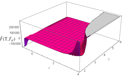
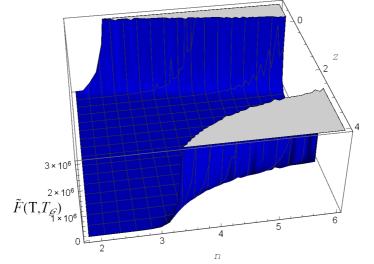
Figure 1: Plots of power-law reconstructed GGPDE $\tilde{F}(T,T_{\mathcal{G}})$ model for $u=2$ (left) and $-2$ (right).

• Now, we investigate stability of the reconstructed GGPDE $\tilde{F}(T,T_{\mathcal{G}})$ model through the squared speed of sound $v_{s}^{2}$ defined as

  $$v_{s}^{2}=\frac{\dot{p}_{\Lambda}}{\dot{\rho}_{\Lambda}}.$$

  The positive value $(v_{s}^{2}>0)$ indicates stability of the model whereas its negative value $(v_{s}^{2}<0)$ corresponds to instability of the model. Using Eqs.(7), (8) and (13) in the above expression, we discuss squared speed of sound parameter graphically. The plots of $v_{s}^{2}$ versus $n$ and redshift parameter $z$ are shown in Figure 2. In the left plot of Figure 2 $(u=2)$, the squared speed of sound parameter is positive showing that the reconstructed $\tilde{F}(T,T_{\mathcal{G}})$ model is stable. For $u=-2$ (right), the corresponding model is not stable at present as well as future epoch.

• The evolutionary behavior of EoS parameter for the reconstructed $\tilde{F}(T,T_{\mathcal{G}})$ model is analyzed by evaluating $\omega_{\Lambda}$ through Eqs.(7) and (8) as follows

  $$\omega_{\Lambda} = -1+(-4\dot{H}-24H^{3}\dot{\mathcal{F}}_{T_{G}}-4\dot{H}\mathcal{F}_{T}-4H\dot{\mathcal{F}}_{T}+(2/3)HT_{G}\dot{\mathcal{F}}_{T_{G}}$$ (14)

  $$+ 8H^{2}\ddot{\mathcal{F}}_{T_{G}})(6H^{2}-\mathcal{F}+12H^{2}\mathcal{F}_{T}+T_{G}\mathcal{F}_{T_{G}}-24H^{3}\dot{\mathcal{F}}_{T_{G}})^{-1}.$$

  Substituting Eq.(13) in the above expression, we obtain the EoS parameters for $u=2$ (Figure 3 left) and $u=-2$ (right) in terms of $z$. We consider same values of the corresponding constants as taken earlier. We investigate the evolution of EoS parameter in the interval $-0.9\leq z\leq 2$ for $n_{1}=3.2$, $n_{2}=4$ and $n_{3}=5$. Figure 3 (left plot) shows that $\omega_{\Lambda}$ starts from phantom region, cuts the phantom divide line and at the end, it becomes zero. This means that EoS parameter shows quintom behavior for $u=2$. Similarly, the right plot represents that $\omega_{\Lambda}$ starts from dust like matter era, passes via quintessence as well as vacuum DE eras and finally enters in the phantom era. Hence, $\omega_{\Lambda}$ behaves like quintom for $u=-2$. In both cases, the reconstructed $\tilde{F}(T,T_{\mathcal{G}})$ model satisfies PDE phenomenon.

• The deceleration parameter $q$ is described as

  $$q=-(\ddot{a}/a)H^{-2}=-\left(1+\dot{H}H^{-2}\right)=\frac{1}{2}+\frac{3}{2}\omega_{\Lambda}.$$ (15)

  

  

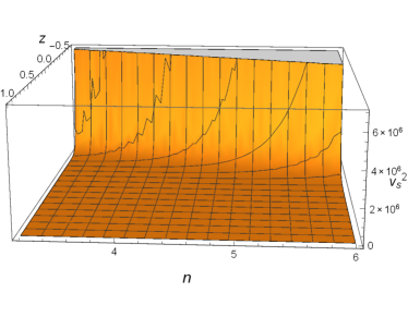
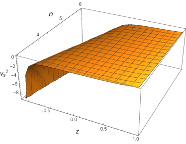
  Figure 2: Plots of power-law $v_{s}^{2}$ for $u=2$ (left) and $-2$ (right).

  

  

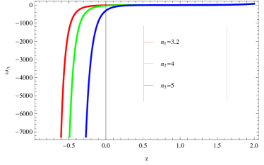
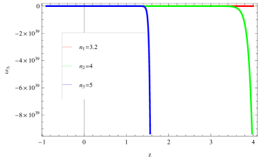
  Figure 3: Plots of power-law EoS parameter $\omega_{\Lambda}$ for $u=2$ (left) and $u=-2$ (right).

  Its positive value indicates decelerating behavior, $q=0$ expresses constant expansion and negative value corresponds to accelerating universe. Substituting the value of $\omega_{\Lambda}$ in the above equation, we obtain deceleration parameter (Figure 4). The left plot for $u=2$ indicates that $q$ attains negative values in the range $-0.9\leq z<0.15$, hence represents accelerating universe in this interval. At $z=0.15$, it becomes zero showing constant behavior and for $z>0.15$, it leads to decelerating universe. In the right plot of Figure 4 $(u=-2)$, the deceleration parameter exhibits negative values in the interval $-0.9\leq z\leq 1.5$ showing accelerating behavior.

• The plane $\omega_{\Lambda}-\omega_{\Lambda^{\prime}}$ is developed for examining different DE models. Initially, Caldwell and Linder [28] used this method to study the behavior of quintessence DE model. They suggested that the covered area in the phase plane corresponds to two regions, thawing region $(\omega_{\Lambda}<0,\omega_{\Lambda^{\prime}}>0)$ as well as freezing region $(\omega_{\Lambda}<0,\omega_{\Lambda^{\prime}}<0)$. Here, we discuss $\omega_{\Lambda}-\omega_{\Lambda^{\prime}}$ plane corresponding to $u=2,-2$ for three different values of $n$. Figure 5 $(u=2)$ shows that $\omega_{\Lambda}-\omega^{\prime}_{\Lambda}$ plane represents thawing regions for all three values of $n$. Similarly, all the curves exhibit the same behavior for $u=-2$ in the interval $-0.9\leq z\leq 1$ as shown in Figure 6. Hence, $\omega_{\Lambda}-\omega^{\prime}_{\Lambda}$ plane shows consistency with the current behavior of the universe for $n=3.2,4$ and $5$.

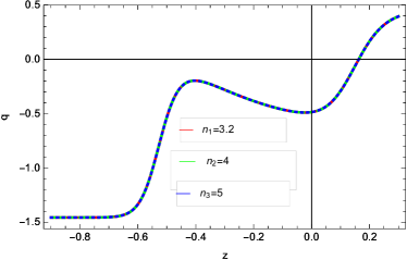
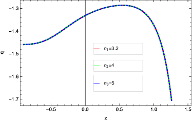
Figure 4: Plots of power-law deceleration parameter $q$ for $u=2$ (left) and $-2$ (right).

• Many DE models have been suggested to understand the phenomenon of DE that ultimately explain the current behavior of the universe. Some of them provide same values of the Hubble and deceleration parameters. Thus it is necessary to determine which one gives better information about acceleration of the expanding universe. For this purpose, Sahni et al. [29] presented two dimensionless parameters named as statefinder parameters and are defined as

  

  

  

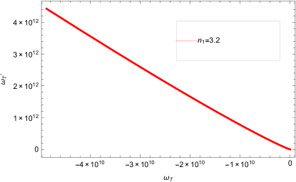
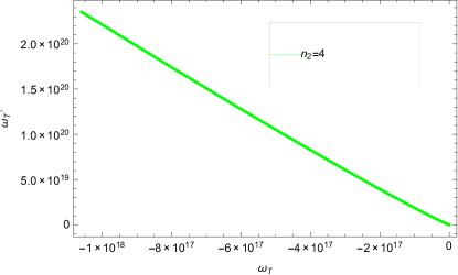
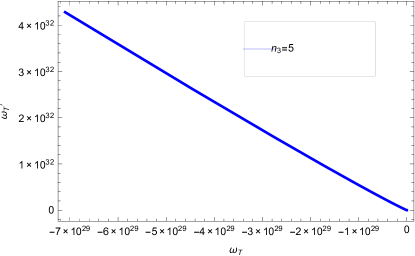
  Figure 5: Plots of power-law $\omega_{\Lambda}-\omega_{\Lambda^{\prime}}$ for $u=2$.

  

  

  

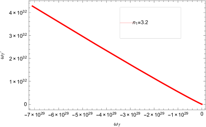
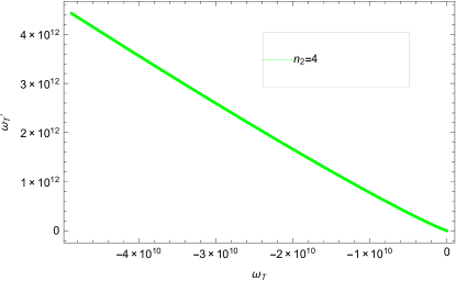
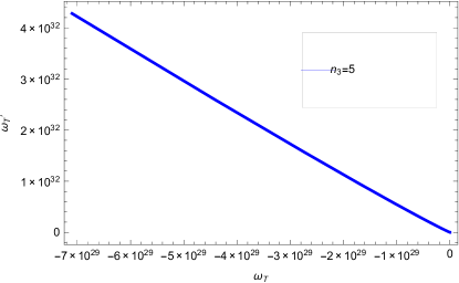
  Figure 6: Plots of power-law $\omega_{\Lambda}-\omega^{\prime}_{\Lambda}$ for $u=-2$.

  $$r=\frac{\dddot{a}}{a}\frac{1}{H^{3}},\quad s=\frac{r-1}{(3q-\frac{3}{2})}.$$

  

  

  

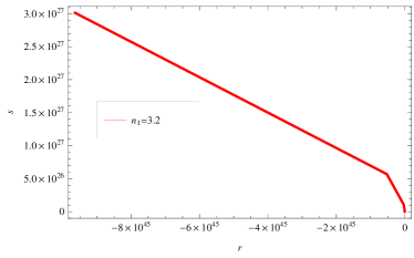
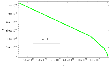
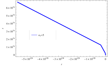
  Figure 7: Plots of power-law $r-s$ plane for $u=2$.

  We can also write the parameter $r$ in terms of $q$ as $r=2q^{2}+q-q^{\prime}$. These parameters describe the well-known cosmic regions such as $(r,s)=(1,1)$ indicating CDM (cold dark matter) limit and $(r,s)=(1,0)$ showing $\Lambda$CDM limit. The region $s>0$, $r<1$ describes phantom and quintessence eras while $s<0$, $r>1$ represents Chaplygin gas model. Here, we establish $r-s$ planes corresponding to our reconstructed GGPDE $\tilde{F}(T,T_{\mathcal{G}})$ models for the same three values of $n$. We assume the same values of corresponding parameters as in the previous section in the range $-0.5\leq z\leq 5$. Figures 7 and 8 show that both reconstructed models for $u=2$ and $-2$ provide the regions of quintessence and phantom DE eras as $s>0$ and $r<1$ for all three values of $n$.

4.2 Scale Factor for the Unified Phases

Now, we investigate the behavior of $\tilde{F}(T,T_{\mathcal{G}})$ models through the scale factor for unified phases. For this purpose, we substitute Eq.(10) in (12) with $a=a_{0}(1+z)^{-1}$ to get a differential equation. We obtain the reconstructed GGPDE $\mathcal{\tilde{F}}(T,T_{\mathcal{G}})$ model in terms of $z$ by solving this differential equation numerically. For both $u=2$ as well as $-2$, we consider $H_{1}=0.9$ and three different values of $H_{2}=2.7,2.75,2.8$. Figure 9 shows that both reconstructed models represent increasing behavior as the value of $z$ increases.

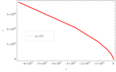
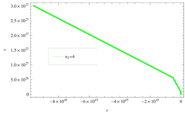
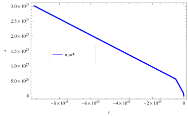
Figure 8: Plots of power-law $r-s$ plane for $u=-2$.

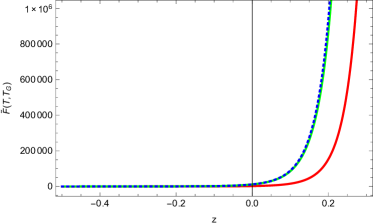
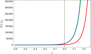
Figure 9: Plots of unified phases reconstructed GGPDE $\tilde{F}(T,T_{\mathcal{G}})$ model for $u=2$ (left) and $-2$ (right). Also, $H_{2}=2.7$ (red), $H_{2}=2.75$ (green) and $H_{2}=2.8$ (blue).

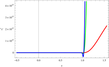
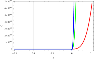
Figure 10: Plots of unified phases $v_{s}^{2}$ for $u=2$ (left) and $-2$ (right). Also, $H_{2}=2.7$ (red), $H_{2}=2.75$ (green) and $H_{2}=2.8$ (blue).

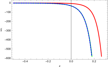
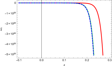
Figure 11: Plots of unified phases EoS parameter $\omega_{\Lambda}$ for $u=2$ (left) and $-2$ (right). Also, $H_{2}=2.7$ (red), $H_{2}=2.75$ (green) and $H_{2}=2.8$ (blue).

• Figure 10 represents the behavior of squared speed of sound parameter for $u=2$ and $-2$. Both plots show that positive values of $v_{s}^{2}$ for $z>1.02$ confirm the stability of $\mathcal{\tilde{F}}(T,T_{\mathcal{G}})$ models.

• Figure 11 indicates that EoS parameter starts from matter dominated era initially ($\omega_{\Lambda}=0$) for $u=2$ as well as $-2$. At $z=0$, $\omega_{\Lambda}$ crosses the phantom divide line for $u=2$ except when $H_{2}=2.7$. For $u=-2$, the EoS parameter remains in the matter dominated era for all values of $H_{2}$ and represents phantom dominated era for $z>2.2$. However, in both cases, the EoS parameter shows consistency with the current expanding behavior of the cosmos as the value of $z$ increases.

• Figure 12 shows deceleration parameter in terms of redshift parameter $z$. This is zero in the interval $-0.9\leq z\leq 1.1$ representing the constant cosmic expansion in both cases $u=2$ as well as $-2$. However, for $z>1.1$, negative values of $q$ give rise to accelerating universe.

• The behavior of $\omega_{\Lambda}-\omega^{\prime}_{\Lambda}$ is shown in Figure 13. The left plot represents freezing region for $H_{2}=2.7$ and $2.75$ while it corresponds to thawing region for $H_{2}=2.8$. In the right plot, $\omega_{\Lambda}-\omega^{\prime}_{\Lambda}$ expresses thawing region for $H_{2}=2.75$ and $2.8$.

• The behavior of statefinder parameters is shown in Figure 14. In the left plot $(u=2)$, we notice that $s<0$, $r>1$ showing Chaplygin gas model while the right plot $(u=-2)$ indicates $s>0$, $r<1$ implying phantom and quintessence eras of the universe.

  

  

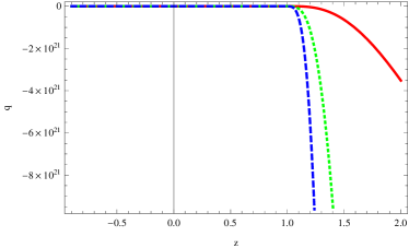
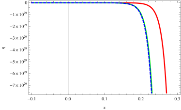
  Figure 12: Plots of unified phases deceleration parameter $q$ for $u=2$ (left) and $-2$ (right). Also, $H_{2}=2.7$ (red), $H_{2}=2.75$ (green) and $H_{2}=2.8$ (blue).

  

  

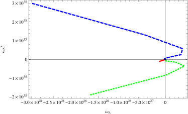
  Figure 13: Plots of unified phases $\omega_{\Lambda}-\omega^{\prime}_{\Lambda}$ for $u=2$ (left) and $-2$ (right). Also, $H_{2}=2.7$ (red), $H_{2}=2.75$ (green) and $H_{2}=2.8$ (blue).

  

  

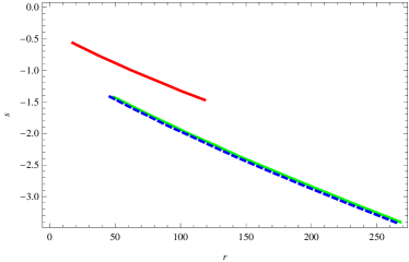
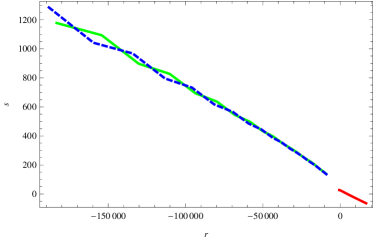
  Figure 14: Plots of unified phases $r-s$ plane for $u=2$ (left) and $-2$ (right). Also, $H_{2}=2.7$ (red), $H_{2}=2.75$ (green) and $H_{2}=2.8$ (blue).

  

  

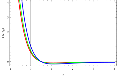
  Figure 15: Plots of intermediate reconstructed GGPDE $\tilde{F}(T,T_{\mathcal{G}})$ model for $u=2$ (left) and $-2$ (right).

  

  

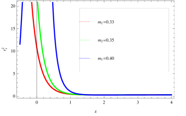
  Figure 16: Plots of intermediate $v_{s}^{2}$ for $u=2$ (left) and $-2$ (right).

  

  

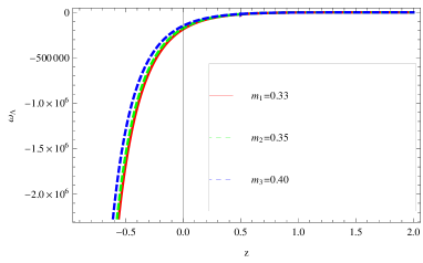
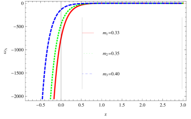
  Figure 17: Plots of intermediate EoS parameter $\omega_{\Lambda}$ for $u=2$ (left) and $-2$ (right). Also, $H_{2}=2.7$ (red), $H_{2}=2.75$ (green) and $H_{2}=2.8$ (blue).

  

  

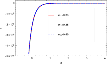
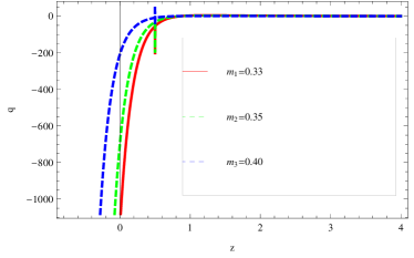
  Figure 18: Plots of intermediate deceleration parameter $q$ for $u=2$ (left) and $-2$ (right). Also, $H_{2}=2.7$ (red), $H_{2}=2.75$ (green) and $H_{2}=2.8$ (blue).

  

  

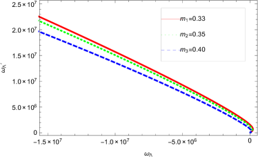
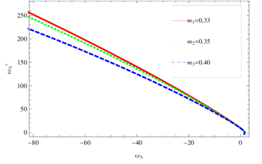
  Figure 19: Plots of intermediate $\omega_{\Lambda}-\omega^{\prime}_{\Lambda}$ for $u=2$ (left) and $-2$ (right).

  

  

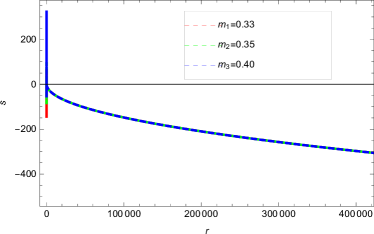
  Figure 20: Plots of intermediate $r-s$ plane for $u=2$ (left) and $-2$ (right).

4.3 Intermediate Scale Factor

For this scale factor, we obtain reconstructed GGPDE $\tilde{F}(T,T_{\mathcal{G}})$ models numerically by using Eq.(11) in (12) as shown in Figure 15. We investigate the behavior of our models by assuming three different values of $m$ as $m_{1}=0.33$, $m_{2}=0.35$, $m_{3}=0.40$ and choose $b=0.1$. The left plot for $u=2$ represents decreasing behavior while the right plot for $u=-2$ expresses increasing behavior.

• Figure 16 confirms the stability of our corresponding model in the range $-0.9\leq z\leq 1.15$ for $u=2$, while for $u=-2$, the model shows instability.

• Figure 17 indicates that for both values of the PDE parameter, the EoS parameter exhibits transition from phantom towards matter dominated era by crossing the phantom divide line for all three values of $m$.

• Figure 18 implies that both plots attain negative values in the range $-0.9\leq z\leq 1.8$ which describe the accelerating behavior of the universe.

• Figure 19 shows the plots for intermediate $\omega_{\Lambda}-\omega^{\prime}_{\Lambda}$ plane that correspond to thawing regions.

• In Figure 20 for $u=2$ (left), we attain the point $(r,s)=(1,0)$ which shows $\Lambda$CDM limit. Also, the statefinder parameters represent phantom and quintessence regions for $0\leq z\leq 1$. On the other hand, these parameters indicate Chaplygin gas model for $1\leq z\leq 2.5$. Similarly, the right plot for $u=-2$ shows Chaplygin gas model.

5 Concluding Remarks

In this paper, we have investigated the behavior of reconstruction models [21] in $\mathcal{F}(T,T_{\mathcal{G}})$ gravity along with GGPDE model as well as three scale factors. For this purpose, we have considered two values of PDE parameter, i.e., $u=2$ and $-2$. We have explored the role of some cosmological parameters versus redshift parameter $z$ in this scenario. We have observed that our models show stability for all the scale factors except power-law and intermediate for $u=-2$. The equation of state parameter in both cases $(u=2,-2)$ represents quintom behavior for all the scale factors. It is found that reconstructed GGPDE $\tilde{F}(T,T_{\mathcal{G}})$ models fulfill the condition of PDE phenomenon. The plot of deceleration parameter versus $z$ exhibits accelerated expansion of the universe.

We have observed that $\omega_{\Lambda}-\omega^{\prime}_{\Lambda}$ plane displays thawing region for power-law as well as intermediate scale factor. The scale factor for two unified phases provides freezing region for $H_{2}=2.8$. The $r-s$ plane shows phantom and quintessence regions for power-law model $(u=2)$ as well as for the scale factor of unified phases $(u=-2)$. For intermediate case, we have achieved $\Lambda$CDM limit. We have found that both the planes, i.e., $\omega_{\Lambda}-\omega_{\Lambda^{\prime}}$ as well as $r-s$ are consistent with the current cosmic behavior.

Sharif and Jawad [17] analyzed GGPDE model by investigating its cosmological consequences in general relativity. Our results are consistent with them for non-interacting case with $\mu=1.55$ and $\nu=1.91$. Jawad and Rani [18] investigated the reconstructed models, their stability and EoS parameter in the modified Horava-Lifshitz $f(\tilde{R})$ gravity. Our results are in great agreement with their work. Sharif and Nazir [19] discussed the same cosmological parameters for GGPDE model in f(T) gravity. We have also compared our results with [19] and found that the EoS parameter and cosmological planes for $u=2$ represent consistency with the same values of model parameters. We have noticed that EoS parameter is also consistent with the observational data [30] given as

$$\omega_{\Lambda} = -1.13^{+0.24}_{-0.25}\quad\text{(Planck +WP+BAO)},$$

$$\omega_{\Lambda} = -1.09\pm 0.17\quad\text{(Planck+WP+Union 2.1)},$$

$$\omega_{\Lambda} = -1.13^{+0.13}_{-0.14}\quad\text{(Planck+WP+SNLS)}.$$

$$\omega_{\Lambda} = -1.24^{+0.18}_{-0.19}\quad\text{(Planck +WP+$H_{0}$)},$$

These constraints have been evaluated by imposing various observational techniques at $95\%$ level of confidence.

References

- [1] Kamenshchik, A.Y., Moschella, U. and Pasquier, V.: Phys. Lett. B 511(2001)265.
- [2] Li, M.: Phys. Lett. B 603(2004)1.
- [3] Cai, R.G.: Phys. Lett. B 657(2007)228.
- [4] Wei, H.: Commun. Theor. Phys. 52(2009)743.
- [5] Sheykhi, A. and Jamil, M.: Gen. Relativ. Gravit. 43(2011)2661.
- [6] Kofinas, G. and Saridakis, E.N.: Phys. Rev. D 90(2014)084044.
- [7] Kofinas, G. and Saridakis, E.N.: Phys. Rev. D 90(2014)084045.
- [8] Kofinas, G., Leon, G. and Saridakis, E.N.: Class. Quantum Grav. 31(2014)175011.
- [9] Waheed, S. and Zubair, M.: Astrophys. Space Sci. 359(2015)47.
- [10] Zubair, M. and Jawad, A.: Astrophys. Space Sci. 360(2015)11.
- [11] Jawad, A.: Eur. Phys. J. Plus 94(2015)130.
- [12] Urban, F.R. and Zhitnitsky, A.R.: Phys. Rev. D 80(2009)063001.
- [13] Cai, R.G., et al.: Phys. Rev. D 86(2012)023511.
- [14] Fernandez, A.R.: Phys. Lett. B 709(2012)313.
- [15] Malekjani, M.: Int. J. Mod. Phys. D 22(2013)1350084.
- [16] Wei, H.: Class. Quantum Grav. 29(2012)175008.
- [17] Sharif, M. and Jawad, A.: Astrophys. Space Sci. 351(2014)321.
- [18] Jawad, A. and Rani, S.: Astrophys. Space Sci. 359(2015)23.
- [19] Sharif, M. and Nazir, K.: Astrophys. Space Sci. 360(2015)57.
- [20] Jawad, A., Rani, S. and Chattopadhyay, S.: Astrophys. Space Sci. 360(2015)37.
- [21] Sharif, M. and Nazir, K.: Mod. Phys. Lett. A 31(2016)1650148.
- [22] Nojiri, S. and Odintsov, S.D.: Gen. Relativ. Gravit. 38(2006)1285.
- [23] Nojiri, S. and Odintsov, S.D.: Phys. Rev. D 74(2006)086005.
- [24] Nojiri, S. and Odintsov, S.D.: Int. J. Geom. Methods Mod. Phys. 4(2007)115.
- [25] Barrow, J.D, Liddle, A.R. and Pahud, C.: Phys. Rev. D 74(2006)127305.
- [26] Nojiri, S. and Odintsov, S.D.: Gen. Relativ. Gravit. 38(2006)1285.
- [27] Jawad, A. and Rani, S.: Adv. High Energy Phys. 2015(2015)952156.
- [28] Caldwell, R.R. and Linder, E.V.: Phys. Rev. Lett. 95(2005)141301.
- [29] Sahni, V., Saini, T.D., Starobinsky, A. A. and Alam, U.: J. Exp. Theor. Phys. Lett. 77(2003)201.
- [30] Ade, P.A.R., et al.: Astron. Astrophys. 571(2014)A16.