Dispersion relation and unphysical poles of Möbius domain-wall fermions in free field theory at finite $L_{s}$

Abstract

We investigate the dispersion relation of Möbius domain-wall fermions in free field theory at finite $L_{s}$. We find that there are $L_{s}-1$ extra poles of Möbius domain-wall fermions in addition to the pole which realizes the physical mode in the continuum limit. The unphysical contribution of these extra poles could be significant when we introduce heavy quarks. We show in this report the fundamental properties of these unphysical poles and discuss the optimal choice of Möbius parameters to minimize their contribution to four-dimensional physics.

1 Introduction

Lattice calculation including the charm quark as well as the lighter quarks is desired to give accurate prediction of the Standard Model, which could play a key role in probing for new physics beyond the Standard Model. Since the charm-quark mass is comparable to currently available lattice cutoffs, the charm quark on the lattice could induce significant discretization errors.

Domain-wall fermions with large input masses are known to have some special difficulties as well as the naïve $O(a)$ discretization errors. Such difficulties were originally suggested Liu:2003kp ; Christ:2004gc by analyzing the eigenvalues of the hermitian version of the domain-wall operator, the five-dimensional Dirac operator multiplied by the chirality operator $\gamma_{5}$ and the five-dimensional reflection operator. That work explained that the hermitian operator involves unphysical modes as well as the physical modes and that the eigenvalues of unphysical modes are largely independent of the input quark mass, while those of physical modes are roughly proportional to the input mass. This implies that the dominance of physical modes would be lost as the input mass increases.

A few years later, Dudek:2006ej observed the oscillatory behavior of correlation functions, which is known as a particular issue of domain-wall fermions and is observed at large values of the domain-wall height such as $M_{5}=1.7$. This oscillatory behavior was described as the result of negative eigenvalues of the transfer matrix Syritsyn:2007mp , which were found to exist at large values of $M_{5}$, $M_{5}>1$ in the case of free field theory.

In this work, we propose another point of view to describe such a curious artifact through an investigation of the pole structure of Möbius domain-wall fermions in free field theory. Although a study of the pole structure of the domain-wall fermion propagator was recently done Liang:2013eoa ; Sufian:2016cft , we find this previous work contains some mistakes in the analytic formula of the quark propagator and the understanding of the pole structure. We provide corrections to these mistakes and discuss the dependence of the pole structure on the domain-wall height $M_{5}$ and the difference between the Möbius parameters $b-c$.

This article is organized as follows. In Section 2, we give definitions and the propagators of Möbius domain-wall fermions both in four and five dimensions. In Section 3, the presence of unphysical poles of domain-wall fermions is demonstrated. In Section 4, we show the energy-momentum dispersion relations for the physical and unphysical poles and discuss their dependence on the parameters of Möbius domain-wall fermions.

2 Definitions and propagator of Möbius domain-wall fermions at finite $L_{s}$

We consider the Möbius domain-wall fermion action $\overline{\psi}D_{\rm MDW}\psi$, where the Dirac operator $D_{\rm MDW}$ in momentum space is given by

$$(D_{\rm MDW})_{s,t}=\tilde{D}\delta_{s,t}-(P_{+}\delta_{s,t+1}+P_{-}\delta_{s,t-1})+m(P_{+}\delta_{s,0}\delta_{t,L_{s}-1}+P_{-}\delta_{s,L_{s}-1}\delta_{t,0}).$$ (1)

Here, we use the chiral projection operators $P_{\pm}=\frac{1}{2}(1\pm\gamma_{5})$ and

$$\tilde{D}=D_{-}^{-1}D_{+},\ \ D_{+}=1+bD_{W},\ \ D_{-}=1-cD_{W},$$ (2)

with the Wilson Dirac operator $D_{W}$ at a negative mass parameter $-M_{5}$,

$$D_{W}={\rm{i}}\hbox to0.0pt{\hbox to5.55557pt{\hfil/\hfil}\hss}\tilde{p}+\sum_{\mu}(1-\cos p_{\mu})-M_{5},$$ (3)

where $\hbox to0.0pt{\hbox to5.55557pt{\hfil/\hfil}\hss}\tilde{p}=\sum_{\mu}\gamma_{\mu}\sin p_{\mu}$. For simplicity, we omit the lattice spacing $a$ and express everything in lattice units throughout this article. As is shown in Brower:2012vk ; Blum:2014tka , if the four-dimensional quark fields are defined as

$$q=P_{-}\psi_{0}+P_{+}\psi_{L_{s}-1},\ \ \overline{q}=\overline{\psi}_{0}P_{+}+\overline{\psi}_{L_{s}-1}P_{-},$$ (4)

the corresponding quark propagator has the form

$$S_{F}^{4d}(p) =P_{-}(D_{\rm MDW}^{-1})_{0,0}P_{+}+P_{+}(D_{\rm MDW}^{-1})_{L_{s}-1,L_{s}-1}P_{-}$$

$$\hskip 11.38109pt+P_{-}(D_{\rm MDW}^{-1})_{0,L_{s}-1}P_{-}+P_{+}(D_{\rm MDW}^{-1})_{L_{s}-1,0}P_{+},$$ (5)

which is the same as the propagator of overlap fermions up to an overall factor and a contact term in the limit of infinite $L_{s}$. Besides the mass parameter, there are four input parameters: the extent of the fifth dimension $L_{s}$, the domain-wall height $M_{5}$, the Möbius parameters $b$ and $c$. Although these parameters characterize the regularization and do not affect any observables in the continuum limit after fermion mass renormalization, discretization errors at finite lattice spacings depend on them.

We can rewrite the five-dimensional Dirac operator $D_{\rm MDW}$ as

$$D_{\rm MDW}={b+c\over D_{-}^{\dagger}D_{-}}{\rm{i}}\hbox to0.0pt{\hbox to5.55557pt{\hfil/\hfil}\hss}\tilde{p}+W^{+}P_{-}+W^{-}P_{+},$$ (6)

where we define

$$W^{\pm}_{s,t} =W\delta_{s,t}-\delta_{s\pm 1,t}+m\delta_{s/t,L_{s}-1}\delta_{t/s,0},$$ (7)

$$W ={-bc(\tilde{p}^{2}+{\cal M}^{2})+(b-c){\cal M}+1\over D_{-}^{\dagger}D_{-}},$$ (8)

$${\cal M} =\sum_{\mu}(1-\cos p_{\mu})-M_{5},$$ (9)

$$D_{-}^{\dagger}D_{-} =c^{2}(\tilde{p}^{2}+{\cal M}^{2})-2c{\cal M}+1,$$ (10)

with $\tilde{p}^{2}=\sum_{\mu}\sin^{2}p_{\mu}$. The five-dimensional propagator of Möbius domain-wall fermions can thus be obtained in the same manner Shamir:1993zy as for Shamir domain-wall fermions:

$$D^{-1}_{\rm MDW} =\left[-{b+c\over D_{-}^{\dagger}D_{-}}{\rm{i}}\hbox to0.0pt{\hbox to5.55557pt{\hfil/\hfil}\hss}\tilde{p}+W^{-}\right]G^{-}P_{-}+\left[-{b+c\over D_{-}^{\dagger}D_{-}}{\rm{i}}\hbox to0.0pt{\hbox to5.55557pt{\hfil/\hfil}\hss}\tilde{p}+W^{+}\right]G^{+}P_{+},$$ (11)

$$G^{\pm}_{s,t} =\left[\bigg{(}{b+c\over D_{-}^{\dagger}D_{-}}\bigg{)}^{2}\tilde{p}^{2}+W^{\mp}W^{\pm}\right]^{-1}_{s,t}$$

$$=A_{0}{\rm{e}}^{-\alpha|s-t|}+A_{\pm}{\rm{e}}^{\alpha(s+t-L_{s}+1)}+A_{\mp}{\rm{e}}^{-\alpha(s+t-L_{s}+1)}+A_{m}\cosh[\alpha(s-t)],$$ (12)

$$\cosh\alpha =\frac{\big{(}{b+c\over D_{-}^{\dagger}D_{-}}\big{)}^{2}\tilde{p}^{2}+W^{2}+1}{2W},$$ (13)

$$A_{0} =\frac{1}{2W\sinh\alpha},$$ (14)

$$A_{\pm} =\frac{A_{0}}{F_{L_{s}}}(1-m^{2})(W-{\rm{e}}^{\mp\alpha}),$$ (15)

$$A_{m} =\frac{A_{0}}{F_{L_{s}}}\left[4mW\sinh\alpha-2(W{\rm{e}}^{-\alpha}-1+m^{2}(1-W{\rm{e}}^{\alpha})){\rm{e}}^{-\alpha L_{s}}\right],$$ (16)

$$F_{L_{s}} ={\rm{e}}^{\alpha L_{s}}(1-W{\rm{e}}^{\alpha}+m^{2}(W{\rm{e}}^{-\alpha}-1))-4mW\sinh\alpha$$

$$\hskip 11.38109pt+{\rm{e}}^{-\alpha L_{s}}(W{\rm{e}}^{-\alpha}-1+m^{2}(1-W{\rm{e}}^{\alpha})).$$ (17)

Inserting this result into (5), we obtain

$$S_{F}^{4d}(p) ={2\sinh(\alpha L_{s})\over F_{L_{s}}}{b+c\over D_{-}^{\dagger}D_{-}}{\rm{i}}\hbox to0.0pt{\hbox to5.55557pt{\hfil/\hfil}\hss}\tilde{p}$$

$$\hskip 11.38109pt+{2\over F_{L_{s}}}\left\{m[W\sinh(\alpha(L_{s}-1))-\sinh(\alpha L_{s})]-W\sinh\alpha\right\}.$$ (18)

3 Unphysical poles at finite $L_{s}$

As is well known, the continuum limit of a lattice fermion reproduces only a relevant Dirac field as long as doublers have been removed. Actual lattice calculations are however carried out at finite lattice spacings, where unphysical extra modes could appear depending on the details of lattice action. Such poles may induce complicated discretization errors which are not easily controlled. In this section, we show the presence of unphysical poles of Möbius domain-wall fermions in free field theory.

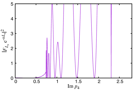
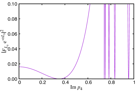
Figure 1: $|F_{L_{s}}{\rm{e}}^{-\alpha L_{s}}|^{2}$ calculated at $L_{s}=8$, $M_{5}=0.9$, $m_{f}^{\rm pole}=0.35$, $b-c=1$, $b+c=1$, $\vec{p}=0$ and ${\rm Re}\leavevmode\nobreak\ p_{4}=0$ plotted as a function of ${\rm Im}\leavevmode\nobreak\ p_{4}$. The lower panels show some magnifications of complicated parts in the top panel, which accommodates all the zero points of $F_{L_{s}}$.

Figure 1 shows $|F_{L_{s}}{\rm{e}}^{-\alpha L_{s}}|^{2}$ calculated at $b=1$, $c=0$, $L_{s}=8$, $M_{5}=0.9$, $\vec{p}=0$ and ${\rm Re}\leavevmode\nobreak\ p_{4}=0$. Here, the input mass parameter $m$ is tuned so that the physical pole mass $m_{f}^{\rm pole}$ reads 0.35. The lower panels show some magnifications of complicated parts in the upper panel, which accommodates all the zero points of $F_{L_{s}}$. Since we find all of the zero points are located on the imaginary axis of $p_{4}$ for this parameter choice, we plot the result only at ${\rm Re}\leavevmode\nobreak\ p_{4}=0$. While the physical pole is seen at ${\rm Im}\leavevmode\nobreak\ p_{4}=m_{f}^{\rm pole}=0.35$, there are nine other zero points of $F_{L_{s}}$. Two of them are identified as the solutions of $\cosh\alpha=1$ or $\cosh\alpha=-1$, which correspond to ${\rm Im}\leavevmode\nobreak\ p_{4}\simeq 2.30$ and 0.74 in the plot, respectively. The other seven zero points are located between these two special zero points.

The special two zero points satisfying $\cosh\alpha=\pm 1$ are not poles of the propagator (18) since the numerator of the propagator also vanishes at these points and the limit $\lim_{\alpha\rightarrow 0,{\rm{i}}\pi}S_{F}^{4d}(p)$ is still finite. On the other hand, the quark propagator at each of the remaining seven zero points is singular, indicating these zero points are unphysical poles. These unphysical poles are located in the region $-1<\cosh\alpha<1$, where $\alpha$ is pure imaginary and therefore any terms in (17) are not suppressed at large values of $L_{s}$, showing some oscillations with varying ${\rm Im}\leavevmode\nobreak\ p_{4}$. Since the number of these oscillations is proportional to $L_{s}$, the number of unphysical poles increases as $L_{s}$ increases and we find $L_{s}-1$ unphysical poles in our analysis.

4 Energy-momentum dispersion relation

As is well known, a pole at $p_{4}=iE$ in Euclidean space behaves $\sim{\rm{e}}^{-Et}$ in coordinate space. If the energy $E$ of the physical pole is close to or larger than that of unphysical poles, the signal of the physical pole may be unclear even at long distances.

The relation between the spatial momentum and the pole energy is represented by the energy-momentum dispersion relation. The dispersion relation on the lattice deviates from that in the continuum limit with $O(a^{2})$ error allowing $O(4)$-violating terms. The dispersion relations for improved overlap fermions using the Brillouin kernel were investigated Cho:2015ffa ; Durr:2017wfi . In this section, we concentrate on unimproved Möbius domain-wall fermions and show the dispersion relation for both the physical and unphysical poles.

Figure 2: Dispersion relation for the domain-wall fermion at $M_{5}=0.9,L_{s}=8,m_{f}^{\rm pole}=0,b+c=1,b-c=1$ and spatial momentum $\vec{p}=({|\vec{p}\,|\over\sqrt{3}},{|\vec{p}\,|\over\sqrt{3}},{|\vec{p}\,|\over\sqrt{3}})$.

Figure 2 shows the dispersion relation for domain-wall fermions at $b=1,c=0$, $M_{5}=0.9$, $L_{s}=8$ and $m_{f}^{\rm pole}=0$. We choose the spatial momentum in the diagonal direction, $\vec{p}=({|\vec{p}\,|\over\sqrt{3}},{|\vec{p}\,|\over\sqrt{3}},{|\vec{p}\,|\over\sqrt{3}})$. At any spatial momenta, there are one physical (solid curve) and seven unphysical poles (dashed curves) on the imaginary axis of $p_{4}$.

As discussed in the previous section, these unphysical poles are located in the region between two curves, $\cosh\alpha=1$ (dashed-dotted curve) and $\cosh\alpha=-1$ (dotted curve). The boundaries $\cosh\alpha=\pm 1$ are analytically given by

$$\cos p_{4}|_{\cosh\alpha=1} =\frac{\sum_{i=1}^{3}\sin^{2}p_{i}+B^{2}+1}{2B},$$ (19)

$$\cos p_{4}|_{\cosh\alpha=-1} =\frac{4+4(b-c)B+(b-c)^{2}(\sum_{i=1}^{3}\sin^{2}p_{i}+B^{2}+1)}{4(b-c)+2(b-c)^{2}B},$$ (20)

$$B =4-M_{5}-\sum_{i=1}^{3}\cos p_{i}.$$ (21)

Note that the solution of $\cosh\alpha=1$, the lower or upper bound on the unphysical poles, depends only on $M_{5}$ and $p_{i}$, while the other bound, the solution of $\cosh\alpha=-1$, depends also on $b-c$. This fact motivates us to vary $b-c$ as well as $M_{5}$, although $b-c$ has not usually been tuned to minimize discretization errors.

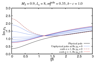
Figure 3: Same as Figure 2 but at $m_{f}^{\rm pole}=0.35$.

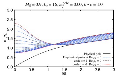
Figure 4: Same as Figure 2 but at $L_{s}=16$.

Before varying $M_{5}$ and $b-c$, which play a key role in determining the region of unphysical pole energies, we briefly show the results of varying the other parameters $m_{f}^{\rm pole}$ and $L_{s}$. Figure 4 shows the result in a massive case at $m_{f}^{\rm pole}=0.35$ with the same values of the other parameters as those in Figure 2. Compared to Figure 2, only the physical pole is supposed to depend significantly on the input mass parameter. The small $m$-dependence of the unphysical poles is compatible with the fact that the boundaries (19) (20) of the unphysical poles are independent of $m$. Therefore, as the physical pole mass $m_{f}^{\rm pole}$ increases, it approaches the unphysical pole masses and the dominance of the physical pole would be lost.

In Figure 4, we show the dispersion relation at $L_{s}=16$. As described in the previous section, $F_{L_{s}}$ oscillates in the region satisfying $-1<\cosh\alpha<1$ with varying $p_{4}$ and the frequency of the oscillation is proportional to $L_{s}$. The number of unphysical poles has therefore increased to 15.

Figure 5: Same as Figure 2 but at $b-c=0.5$.

Figure 6: Same as Figure 2 but at $b-c=0$.

Figure 6 shows the result at $b-c=0.5$. In the plot, one bound on the unphysical poles satisfying $\cosh\alpha=-1$ is larger than that for the Shamir type $b-c=1$ and the lightest unphysical pole mass has been increased to $\sim 1.41$, implying that the contribution of unphysical poles at long distances would be suppressed more rapidly. In Figure 6, which shows the result at $b-c=0$, the curve of $\cosh\alpha=-1$ is infinitely large as (20) indicates. Thus, small values of $b-c$ make the unphysical modes heavy and would realize a small contribution of unphysical poles to four-dimensional physics.

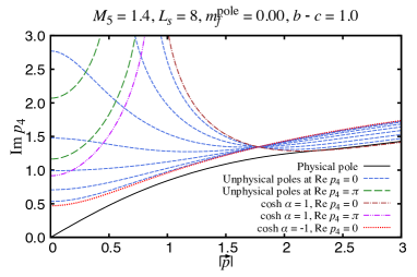
Figure 7: Same as Figure 2 but at $M_{5}=1.4$.

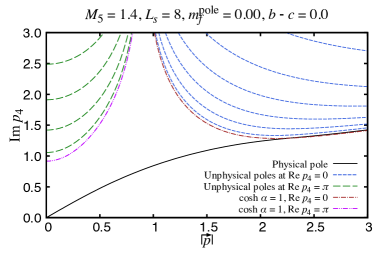
Figure 8: Same as Figure 8 but at $b-c=0$.

So far, we have discussed the case of $M_{5}=0.9$, in which unphysical poles are located only on the imaginary axis of $p_{4}$. If $M_{5}>1$, $\alpha$ could be pure imaginary at ${\rm Re}\leavevmode\nobreak\ p_{4}=\pi$ as well as at ${\rm Re}\leavevmode\nobreak\ p_{4}=0$ and therefore some of the unphysical poles may exist at ${\rm Re}\leavevmode\nobreak\ p_{4}=\pi$. Figure 8 shows the result at $M_{5}=1.4$. There are two separated curves of $\cosh\alpha=1$, which blow up at $|\vec{p}\,|\simeq 0.90$. One of them at smaller spatial momenta (dashed double-dotted curve) is located at ${\rm Re}\leavevmode\nobreak\ p_{4}=\pi$. As suggested in Liang:2013eoa ; Sufian:2016cft , unphysical poles at ${\rm Re}\leavevmode\nobreak\ p_{4}=\pi$ may cause unphysical oscillation since the contribution of a pole at $p_{4}=p_{4}^{\rm pole}$ to the quark propagator for the time direction has a term $\sim{\rm{e}}^{{\rm{i}}p_{4}^{\rm pole}x_{4}}$, which is oscillatory unless ${\rm Re}\leavevmode\nobreak\ p_{4}^{\rm pole}=0$. In Figure 8, the lower bound on the unphysical pole masses at ${\rm Re}\leavevmode\nobreak\ p_{4}=0$ ($\cosh\alpha=-1$) is smaller than that at ${\rm Re}\leavevmode\nobreak\ p_{4}=\pi$ ($\cosh\alpha=1$), indicating that the unphysical contributions from the former type of poles may be more significant than those from the latter type of poles. Figure 8 shows the result at $b-c=0$. Since the boundary of $\cosh\alpha=-1$ goes to infinity at $b-c=0$, there are no unphysical poles on the imaginary axis of $p_{4}$ at small spatial momenta ($|\vec{p}\,|\lesssim 0.90$). All unphysical poles are located at ${\rm Re}\leavevmode\nobreak\ p_{4}=\pi$ for $|\vec{p}\,|\lesssim 0.90$ and at ${\rm Re}\leavevmode\nobreak\ p_{4}=0$ for $|\vec{p}\,|\gtrsim 0.90$.

As we have seen, the lower bound on the unphysical pole energies can be increased by taking $b-c$ smaller when $p_{4}|_{\cosh\alpha=-1}<p_{4}|_{\cosh\alpha=1}$. Since $b-c=1$ satisfies this inequality at zero and small spatial momenta, this fact implies that we can reduce the contamination of unphysical poles by decreasing $b-c$ from 1 at least in free field theory. Non-perturbative effects may slightly change this prospect and this possibility motivates us to implement a non-perturbative study on the effect of unphysical poles, which is on-going.

5 Summary

We have shown that the propagator of domain-wall fermions has $L_{s}-1$ extra poles. Since the energy-momentum dispersion relation for unphysical poles is mostly independent of input physical quark mass, these poles may affect 4D physics significantly when the input quark mass is comparable to the unphysical pole masses, which is $O(a^{-1})$. Examining the dependence on parameters of Möbius domain-wall fermions, we demonstrate that $b-c$ should be smaller than 1 for a rapid suppression of the contamination of unphysical poles at least in free field theory.

It should be also noted that small values of $b-c$ may spoil the approximation of the sign function because the upper limit on the eigenvalues of the Möbius kernel becomes large. Therefore, we need to tune the parameters taking account of the violation of the Ginsparg-Wilson relation as well as of the effects of unphysical poles. A non-perturbative study to tune the parameters of Möbius domain-wall fermions is on-going. The property of unphysical poles is discussed in the full paper Tomii:2017lyo in more detail.

References

- (1) G.f. Liu, Ph.D. thesis, Columbia U. (2003)
- (2) N.H. Christ, G. Liu, Nucl. Phys. Proc. Suppl. 129, 272 (2004)
- (3) J.J. Dudek, R.G. Edwards, D.G. Richards, Phys. Rev. D73, 074507 (2006), hep-ph/0601137
- (4) S. Syritsyn, J.W. Negele, PoS LAT2007, 078 (2007), 0710.0425
- (5) J. Liang, Y. Chen, M. Gong, L.C. Gui, K.F. Liu, Z. Liu, Y.B. Yang, Phys. Rev. D89, 094507 (2014), 1310.3532
- (6) R.S. Sufian, M.J. Glatzmaier, Y.B. Yang (2016), 1603.01591
- (7) R.C. Brower, H. Neff, K. Orginos (2012), 1206.5214
- (8) T. Blum et al. (RBC, UKQCD), Phys. Rev. D93, 074505 (2016), 1411.7017
- (9) Y. Shamir, Nucl. Phys. B406, 90 (1993), hep-lat/9303005
- (10) Y.G. Cho, S. Hashimoto, A. JÃttner, T. Kaneko, M. Marinkovic, J.I. Noaki, J.T. Tsang, JHEP 05, 072 (2015), 1504.01630
- (11) S. Durr, G. Koutsou (2017), 1701.00726
- (12) M. Tomii, Phys. Rev. D96, 074504 (2017), 1706.03099