NNDrone : a toolkit for the mass application of machine learning in High Energy Physics

Abstract

Machine learning has proven to be an indispensable tool in the selection of interesting events in high energy physics. Such technologies will become increasingly important as detector upgrades are introduced and data rates increase by orders of magnitude. We propose a toolkit to enable the creation of a drone classifier from any machine learning classifier, such that different classifiers may be standardised into a single form and executed in parallel. We demonstrate the capability of the drone neural network to learn the required properties of the input neural network without the use of any labels from the training data, only using appropriate questioning of the input neural network.

1 Introduction

Data-collection rates in high energy physics (HEP) experiments, particularly those at the Large Hadron Collider (LHC), are a continuing challenge and resulting datasets require large amounts of computing power to process. For example, the LHCb experiment [1] processes an event rate of 1${\rm\,MHz}$ in a software-based trigger [2]. The purpose of this trigger is to reduce the output data rate to manageable levels, i.e. to fit in the available storage resources offline. This amounts to a reduction from 60 GB per second to an output data rate of 0.6 GB per second. In order to accomplish such a remarkable real-time data reduction in the software based trigger, novel ideas have been introduced, such as the real-time alignment and calibration of the detector [3], in addition to the concept of real-time analysis [4], whereby a subset of the particles from the proton collisions need only be saved, and not the raw data from the sub-detectors. The aforementioned data-reduction strategy is similar across all LHC experiments, where software based selections are applied in low-latency environments.

Machine learning (ML) is becoming an increasingly important tool to filter datasets, be it with the identification of interesting event topologies, or the distinction between individual particle species. For the case of LHCb data-taking, over 600 unique signatures are searched for in parallel in real time, each with its own set of requirements. However only a handful at present make use of machine learning.

A large ecosystem is available for analysts to create machine learning classifiers; the TMVA [5] and Neurobayes [6] tools being among the most widely used. More recent examples gaining popularity include Scikit-Learn [7] and Keras [8]. It has been proven in many LHC analyses that ML classifiers account for differences in the correlations of training variables between signal and background events, therefore enabling more powerful data reduction. Despite this, the majority of searches for interesting signatures are performed without the use of ML classifiers. Often the reason for this is the relative difficulty in the implementation of a preferred ML classifier to the C++/Python combination of event selection frameworks [9]. Another reason is the required algorithm speed. Methods such as Bonsai Boosted Decision Trees (BBDTs) [10] have been developed in order to enable the quick evaluation of models. The BBDT approach relies on the discretization of inputs such that all possible combinations along with the associated classifier response is known before the model is evaluated. One potential drawback of the BBDT approach is that the number of input variables is limited in order to limit the number of possible combinations.

We present in this article a package that allows an analyst to train a drone neural network that learns the important features of a given ML learning classifier from any chosen package such as SciKit-Learn or Keras. The resulting parameters are then fed into a C++ algorithm that performs execution in HEP production environments. The details of the drone training are provided in Sec. 2. This is followed by real examples using simulated data in Sec. 3. The advantages of the approach are discussed in Sec. 4 and a summary is provided in Sec. 5.

2 Drone learning

The training of the drone network requires that the original network is extensively probed in the parameter space in which accuracy is desired. The principle utilised in the training of the drone is that sufficient approximation of the original network is achieved with sufficient expansion of the hyperparameter space of the drone, and that the same global minimum of the loss function can be found, as reported in Ref. [11]. The ability of a neural network with a continuous, bounded, non-constant activation function to approximate functions to an arbitrary degree has been indeed known since the early 1990s [12].

2.1 Initial drone structure and corresponding training

The drone chosen for use in this article is initialised as a neural network with a single intermediate (hidden) layer of 5 nodes using a standard sigmoid activation function. The network has the number of inputs determined from the number of desired characteristics of the decay signature. A single output is taken from the network and a linear model is used to relate layers.

The model is made to approximate the original classifier through a supervised learning technique, though not in the traditional sense. Instead of a label as signal or background taken from the training data, the output of the original classifier is used as a label. This means that the loss function is defined as

$$\mathcal{L}=\sum_{i}\left(F(\vec{x}_{i})-G_{i}(\vec{x}_{i})\right)^{2},$$ (1)

where $F(\vec{x}_{i})$ and $G(\vec{x}_{i})$ are the outputs of the original and drone models on datapoint $i$ of the mini-batch, respectively. The advantage of such a loss function is per-event equivalence of the original and drone model, in addition to equivalence of performance. For the drone training detailed in this article, standard mini-batch stochastic gradient descent is used. A feature of this method is that the drone classifier does not see the labels of the training data, but rather learns the same properties from the original classifier. This is therefore a neural network that learns from another neural network in an empirical manner.

2.2 Model morphing during the learning phase

In order to keep the hyperparameter space to the minimum required level, additional degrees of freedom are added only when required. This removes the possibility of choosing an incorrect size of the drone network. During the learning phase, the following conditions are required to trigger the extension of the hidden layer in the $j^{\rm th}$ epoch:

$$\delta_{j} \equiv|\mathcal{L}_{j}-\mathcal{L}_{j-1}|/\mathcal{L}_{j}<\kappa,$$ (2)

$$\sigma_{j} \equiv m(1-e^{-b(\hat{t}+n)})\delta_{j}\mathcal{L}_{j}$$

$$\mathcal{L}_{j} <\hat{\mathcal{L}}-\sigma_{j},$$ (3)

where $\kappa$ is the required threshold, $\sigma$ is the required minimum improvement of the loss function and $\hat{\mathcal{L}}$ is the value of the loss function when the hidden layer was last extended. The required improvement starts from a minimum at $n$, increases with epoch number after previous extension $\hat{t}$ and steepness $b$ until a maximum at $m$. The precise values of the parameters $\kappa$, $n$, $m$, $b$ are not of particular importance. Rather, the topology described by eqs. 2 and 3 is crucial. The relative loss function improvement, $\delta_{j}$, can never realistically be larger than $1$ and the limit, $\kappa$, at which no significant improvement occurs is acceptably set at 0.02 (smaller than $2\sigma$ standard deviations). The descent in loss space, $\hat{\mathcal{L}}-\mathcal{L}_{j}$, is further required to be significantly large, minimizing the chance of getting stuck in isolated local minima. The function, $\sigma_{j}$, is chosen to increase this requirement with each epoch for two reasons - it is bounded and can approach its asymptote arbitrarily fast. It scales $\delta_{j}$ such that the loss descent must be significant before an update is triggered. Since $\delta_{j}$ is expected to decrease with epoch number, the minumum and maximum values of $\sigma_{j}$ are chosen as such:

$$\sigma_{j}(\hat{t}=0) \equiv min(\sigma_{j})\equiv 2.5\delta_{j}\mathcal{L}_{j}\implies 5\sigma~{}\text{std.dev.}$$ (4)

$$\sigma_{j}(\hat{t}=\infty) \equiv min(\sigma_{j})\equiv 25\delta_{j}\mathcal{L}_{j}\implies 50\sigma~{}\text{std.dev.}$$ (5)

The steepness, $b$, is chosen such that the transition from the minimum to maximum takes on average 50 epochs. This ensures a change cannot be triggered immediately after a previous one and the learning can still proceed if more freedom is indeed required. Also, it allows the network to stabilize after a big change.

When the conditions in eqs. 2 and 3 are met, the linear model is updated to extend the weights matrices and bias vectors to accommodate the layer addition. The associated neurons are initialised with a zero weight to ensure continuity of the loss function value.

3 High energy physics applications

3.1 B physics

3.1.1 Data sample

In order to demonstrate the functionality of the toolkit, data samples generated from the RapidSim package [13] are used. The interesting signal is chosen to be the ${{B}^{0}_{s}}\rightarrow{{J\mskip-3.0mu/\mskip-2.0mu\psi\mskip 2.0mu}}(\rightarrow\mu\mu)\phi(\rightarrow KK)$ decay, and the background is the ${{D}^{0}}\rightarrow\pi\pi\pi\pi$ decay. A total of 10000 candidates is generated for each decay.

3.1.2 Training of the original classifier

The machine learning classifier, using the Keras framework [8, 14], is constructed as a locally connected first layer (in which filters are applied to different regions in contrast to a full convolution layer), followed by a pooling layer, and a standard dense layer. The exact definition can be found below.

⬇

classifier = Sequential()

classifier.add(LocallyConnected1D(

filters = 90, kernel_size = 2,

activation = ’sigmoid’,

input_shape = (len(setTrain[0]), 1)))

classifier.add(GlobalMaxPooling1D())

classifier.add(Dense(30, activation = ’sigmoid’))

classifier.add(Dense(1, activation = ’sigmoid’))

classifier.compile(optimizer = ’adam’,

loss = ’binary_crossentropy’

, metrics = [’accuracy’])

The neural network is trained using kinematic properties of the respective decays. These include the pseudorapidity, $\eta$, and momentum transverse to the direction of the input proton beams, $p_{\rm T}$, of the decaying particle. In addition, the minimum and maximum $p_{\rm T}$ and $\eta$ of the final state particles is used. The signal and background distributions of the input variables are shown in Fig. 1.

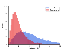
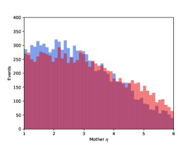
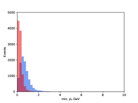
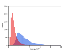
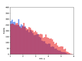
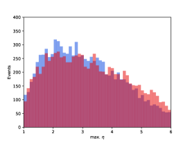
Figure 1: Comparison of the signal and background distributions used to train the Keras B decay classifier.

In the training of the original classifier, half of the data is reserved in order to test for overtraining.

3.2 Jet separation

3.2.1 Data sample

A further demonstration is provided demonstrating a classifiers ability to separate different kinds of jets. The data sample to show this has been generated from Pythia [15] simulating pp collisions at 14$\mathrm{\,Te\kern-1.00006ptV}$. The jets themselves are reconstructed in the Rivet analysis framework [16] and are created using the FastJet [17] package using the $K_{t}$ algorithm [18] (the definition of the $K_{t}$ variable and a review of jet reconstruction algorithms may be found in Refs [19] and [20] respectively). A jet $p_{\rm T}$ requirement of 20$\mathrm{\,Ge\kern-1.00006ptV}$ is imposed on all jets. All other parameters remain at the default values for Rivet version 2.5.4. The signal sample is chosen to correspond to a $qg\rightarrow Wq$ type of interaction, whereas the background is chosen to correspond to a $gg\rightarrow gg$ type. These correspond to the Rivet analyses named MC_WJETS and MC_QCD, respectively. Jets that originate from gluons in the final state form a background to many analyses, therefore efficient rejection of such processes is important in making measurements [21].

3.2.2 Training of the original classifier

The machine learning classifier chosen is also a Keras-based convolutional neural net, constructed in an similar way as described in Sec 3.1.2

⬇

classifier = Sequential()

classifier.add(LocallyConnected1D(

filters = 90, kernel_size = 2,

activation = ’sigmoid’,

input_shape = (len(setTrain[0]), 1)))

classifier.add(GlobalMaxPooling1D())

classifier.add(Dense(30, activation = ’sigmoid’))

classifier.add(Dense(1, activation = ’sigmoid’))

classifier.compile(optimizer = ’adam’,

loss = ’binary_crossentropy’

, metrics = [’accuracy’])

The training data is based around the properties of the measured jets. The list of features taken consists of the azimuthal angle, $\phi$, $\eta$ of the jet; the spread of neutral and hadronic contributions to the jet in the $\phi$, $\eta$ variables, along with average and energy weighted kinematic variables. In total 17 different features are used. The signal and background distributions of the input variables are shown in Fig. 2.

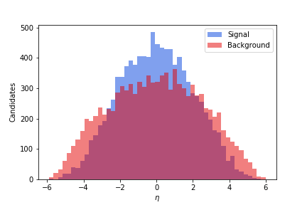
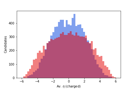
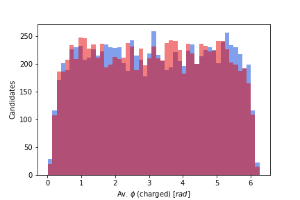
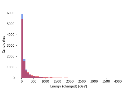
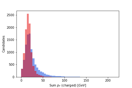
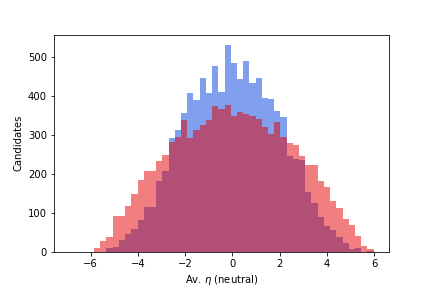
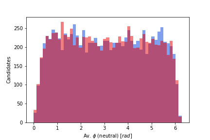
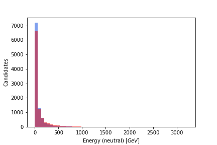
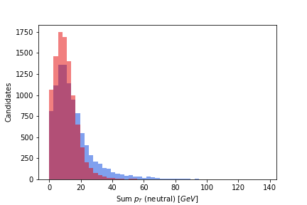
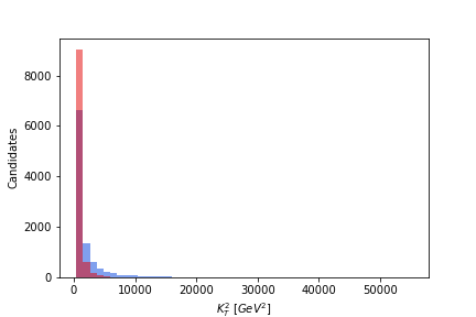
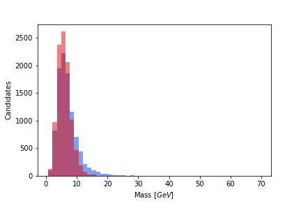
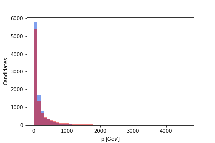
Figure 2: Comparison of the signal and background distributions used to train the Keras jet separation classifier.

3.3 Drone conversions

The drone neural networks are trained following the procedure outlined in Sec. 2, In total, 300 epochs are used with the learning rate of the stochastic gradient descent set to 0.05. The value of $\kappa$ is chosen to be 0.02, the value of $b$ is chosen to be 0.04 and the value of $m$ is chosen to be 50.

The loss history of the drone approximations are shown in Fig. 3 as a function of epoch number. The convergence is also shown in Fig. 4, which shows the difference in the value of the loss function with respect to the previous epoch. The epochs that trigger an increase in the number of hyperparameters are also overlaid. In total for the case of B decays and for the case of the jet separation classifier, an increase was triggered 10 times. The total number of parameters in the final drone neural networks are therefore 121 and 286 for the B decay drone and the jet separation drone, respectively. It is interesting to note that with the algorithm design of Sec. 2, the introduction of the new parameter space causes the drone networks to learn faster, as evidenced by increases in Fig. 4 with continuing descent of the loss functions. The performance of the original classifiers compared to the drone classifiers are shown in Figure 5.

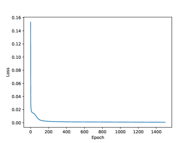
Figure 3: Convergence of the loss function during the drone training for the case of the B decay (left) and jet separation (right) examples.

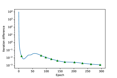
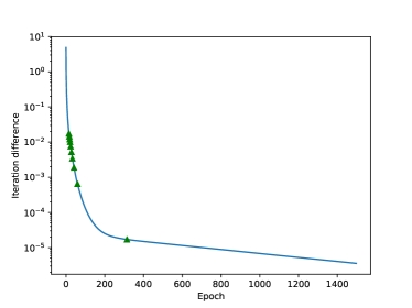
Figure 4: Difference in the loss function with respect to the previous iteration for the case of the B decay (left) and jet separation (right) examples. The green triangles depict the epoch number in which the number of hyperperameters was increased.

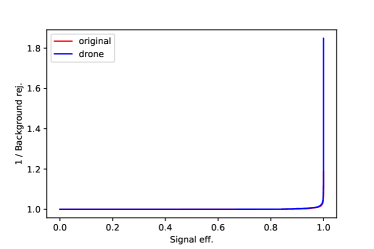
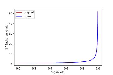
Figure 5: Signal efficiency versus background rejection of the original classifier (red) and drone approximation (blue) for the case of the B decay (left) and jet separation (right) examples.

4 Drone storage and transferability and suitability for low-latency environments

The hyperparameters and structure of the drone are required to be portable and easily stored for later usage. For this the JSON format was chosen as mediator. It is human-readable and easily accessible in the Python and C++ environments commonly used in HEP. Thus, it is readily deployable in both personal and production environments.

Provided is a tool to export and save a drone neural network to a JSON formatted file which preserves the input & output structure, the layers and nodes, all hyperparameters and activation functions. The drone configuration is later read in by an equivalent tool into the production software framework, which then constructs a class object based on the Keras model. The C++ class implements a flexible member structure that is capable of completely reproducing the original drone. The production implementation may be used for all data reduction levels, be it in the form of a low-latency trigger for example up to the latest stages of data handling and output.

A major advantage of this method is that analysts and users have the full freedom of latest developments of industry standards, but need only to support a more manageable implementation in the low-latency software. This is further aided by projects such as ONNX [22], which enable classifiers from a wider range of software packages to be converted to a framework in which an approximation converter is available.

The identical performance show in Fig. 5 is clearly the ideal scenario, even though such good agreement is not always required to give better results than other low-latency methods. However it is worth noting that the drones created in the examples of Sec. 3 are faster to evaluate. The comparison of the time taken for each model evaluation, determined from a desktop using a Intel Core i5-7267U processor is shown in Table 2.

Table 1: Hyperparameter number comparisons of the original models and drone approximations for the HEP examples.

	original model	drone
B decay	4,111	121
jet separation	7081	286

Table 2: Processing time comparisons of the original models and drone approximations for the HEP examples.

	original model	drone
B decay	$3.87\times 10^{-4}$ s	$4.8\times 10^{-5}$ s
jet separation	$4.79\times 10^{-4}$ s	$6.2\times 10^{-5}$ s

5 Summary

It has been demonstrated that for the case of a high energy physics event selection application, a drone neural network is able to accurately approximate and learn the features of a neural network with a different structure. The proposed algorithm design allows the drone to learn the aforementioned features without ever having access to the training data, or indeed any data, but only with appropriate questioning of the original model.

The equivalency of the outputs of the drone and original model enables an analyst to treat both the original and the drone in the same way. The creation of a drone in a standardised form permits an analyst to use any desired machine-learning package to isolate a decay signature, and from this create a classifier guaranteed to be suitable for execution in the C++ real-time data selection frameworks.

References

- [1] A. A. Alves Jr., et al., The LHCb detector at the LHC, JINST 3 (2008) S08005. doi:10.1088/1748-0221/3/08/S08005.
- [2] R. Aaij, et al., LHCb detector performance, Int. J. Mod. Phys. A30 (2015) 1530022. arXiv:1412.6352, doi:10.1142/S0217751X15300227.
- [3] Z. Xu, M. Tobin, Novel real-time alignment and calibration of the LHCb detector in Run II, Nucl. Instrum. Meth. A824 (2016) 70–71. doi:10.1016/j.nima.2015.11.040.
- [4] R. Aaij, et al., Tesla : an application for real-time data analysis in High Energy Physics, Comput. Phys. Commun. 208 (2016) 35–42. arXiv:1604.05596, doi:10.1016/j.cpc.2016.07.022.
- [5] A. Hocker, et al., TMVA - Toolkit for Multivariate Data Analysis, PoS ACAT (2007) 040. arXiv:physics/0703039.
- [6] M. Feindt, U. Kerzel, The NeuroBayes neural network package, Nucl. Instrum. Meth. A559 (2006) 190–194. doi:10.1016/j.nima.2005.11.166.
- [7] F. Pedregosa, et al., Scikit-learn: Machine Learning in Python, J. Machine Learning Res. 12 (2011) 2825–2830. arXiv:1201.0490.
- [8] F. Chollet, et al., Keras, https://github.com/fchollet/keras (2015).
- [9] G. Barrand, et al., GAUDI - A software architecture and framework for building HEP data processing applications, Comput. Phys. Commun. 140 (2001) 45–55. doi:10.1016/S0010-4655(01)00254-5.
- [10] V. V. Gligorov, M. Williams, Efficient, reliable and fast high-level triggering using a bonsai boosted decision tree, JINST 8 (2013) P02013. arXiv:1210.6861, doi:10.1088/1748-0221/8/02/P02013.
-
[11]
A. Choromanska, M. Henaff, M. Mathieu, G. B. Arous, Y. LeCun,
The loss surface of multilayer
networks, CoRR abs/1412.0233.
arXiv:1412.0233.
URL http://arxiv.org/abs/1412.0233 -
[12]
K. Hornik,
Approximation
capabilities of multilayer feedforward networks, Neural Networks 4 (2)
(1991) 251 – 257.
doi:10.1016/0893-6080(91)90009-T.
URL http://www.sciencedirect.com/science/article/pii/089360809190009T - [13] G. A. Cowan, D. C. Craik, M. D. Needham, RapidSim: an application for the fast simulation of heavy-quark hadron decays, Comput. Phys. Commun. 214 (2017) 239–246. arXiv:1612.07489, doi:10.1016/j.cpc.2017.01.029.
-
[14]
D. P. Kingma, J. Ba, Adam: A method for
stochastic optimization, CoRR abs/1412.6980.
arXiv:1412.6980.
URL http://arxiv.org/abs/1412.6980 - [15] T. Sjöstrand, S. Mrenna, P. Skands, A brief introduction to PYTHIA 8.1, Comput. Phys. Commun. 178 (2008) 852–867. arXiv:0710.3820, doi:10.1016/j.cpc.2008.01.036.
- [16] A. Buckley, J. Butterworth, L. Lonnblad, D. Grellscheid, H. Hoeth, J. Monk, H. Schulz, F. Siegert, Rivet user manual, Comput. Phys. Commun. 184 (2013) 2803–2819. arXiv:1003.0694, doi:10.1016/j.cpc.2013.05.021.
- [17] M. Cacciari, G. P. Salam, G. Soyez, FastJet User Manual, Eur. Phys. J. C72 (2012) 1896. arXiv:1111.6097, doi:10.1140/epjc/s10052-012-1896-2.
- [18] G. P. Salam, G. Soyez, A Practical Seedless Infrared-Safe Cone jet algorithm, JHEP 05 (2007) 086. arXiv:0704.0292, doi:10.1088/1126-6708/2007/05/086.
- [19] S. Catani, Y. L. Dokshitzer, M. H. Seymour, B. R. Webber, Longitudinally invariant clustering algorithms for hadron hadron collisions, Nucl. Phys. B406 (1993) 187–224. doi:10.1016/0550-3213(93)90166-M.
- [20] R. Atkin, Review of jet reconstruction algorithms, J. Phys. Conf. Ser. 645 (1) (2015) 012008. doi:10.1088/1742-6596/645/1/012008.
- [21] P. T. Komiske, E. M. Metodiev, M. D. Schwartz, Deep learning in color: towards automated quark/gluon jet discrimination, JHEP 01 (2017) 110. arXiv:1612.01551, doi:10.1007/JHEP01(2017)110.
-
[22]
ONNX: Open Neural Network Exchange Format.
URL http://onnx.ai