Distribution Amplitudes of Heavy Hadrons:
Theory and Applications

Abstract

The physics of heavy quarks becomes a very reach area of study thanks to an excellent operation of hadron colliders and $B$-factories and exciting results from them. Experimental data obtained allows to get some information about the heavy hadron dynamics. In this case, the models for the heavy hadron wave-functions are required to do theoretical predictions for concrete processes under study. In many cases, the light-cone description is enough to obtain theoretical estimates for heavy hadron decays. A discussion of the wave-functions of the $B$-meson and heavy bottom baryons in terms of the light-cone distribution amplitudes is given in this paper. Simple models for the distribution amplitudes are presented and their scale dependence is discussed. Moments of the distribution amplitudes which are entering the branching fractions of radiative, leptonic and semileptonic $B$-mesons decays are also briefly discussed.

1 Introduction

Physics of heavy hadrons, both experimental and theoretical, still remains a hot topic at present. From one side, the remarkable operation of the hadron collider LHC at CERN provides us with a lot of interesting and exciting results and, from the other side, many more results can be obtained from the $B$-factory at KEK which is under construction now and hopefully to be run in a year from now. Among the excellent achievements obtained at the LHC, there is the measurement of the rare purely leptonic decay $B_{s}\to\mu^{+}\mu^{-}$ by the LHCb and CMS collaborations [1] in a nice agreement with the theoretical expectations based on the Standard Model (SM) (see, for example, [2] and reference therein) and the evidence of the similar decay $B^{0}\to\mu^{+}\mu^{-}$ seen by the same collaborations [1] is also in agreement with the SM predictions [2]. Let us note that both decays were considered as a clean candle into possible new physics at the flavor-physics frontue, when predicted branching fractions are substantially larger the SM expectations. At the statistics have been already collected at the LHC, it starts possible to make a detail combine analysis of the rare $B\to K^{(*)}\ell^{+}\ell^{-}$ decays, where $\ell=e,\,\mu$, in the lepton-pair invariant mass squared and spherical angles. In particular, some quantities show a sizable deviation from theoretical predictions and these require theoretical explanation. The other semileptonic decay $B^{+}\to\pi^{+}\mu^{+}\mu^{-}$ have been also observed at the LHC [3] and, on the Run-II statistics, for the first time partially integrated branching fraction over the lepton-pair invariant mass divided into 8 bins have been experimentally obtained [4] in a good agreement with the SM predictions. All these results need to be approved at the $B$-factory SuperKEKB after its operation will start and, in addition, one should wait new exciting results as several $B$-meson decay modes, being unobservable at the LHC, can be measured by the Belle collaboration and are of great importance to get a complete picture of $B$-meson physics. Among them, one can specify the decays like $B\to K^{(*)}\nu\bar{\nu}$ and $B^{0}\to\pi^{0}\ell^{+}\ell^{-}$.

In a difference to $B$-meson decays, the situation with bottom baryons is a little bit worser as the SuperKEKB machine is not designed for the $\Lambda_{b}$ and heavier baryon production. So, the LHC is the only source for the bottom-baryon study for quite some time. As the result, only limited information about this part of the hadronic sector is available and a lot of theoretical predictions will wait their check for future experimental facilities. Interesting processes are the rare semileptonic decays $\Lambda_{b}\to\Lambda\ell^{+}\ell^{-}$ decays, where $\ell=e,\,\mu$, which are the baryonic realization of the flavor-changing neutral current transition $b\to s\ell^{+}\ell^{-}$, quite sensitive to induced by loop diagrams contributions from new physics.

Theoretical predictions for weak decays require some information about the dynamics of light quarks in heavy hadrons — $B_{(s)}$-meson and bottom baryon. Several approaches have been already worked out and, in some cases, experimentally checked like $B\to K^{(*)}\ell^{+}\ell^{-}$ decays, where $\ell=e,\,\mu$, both at $B$-factories at SLAC and KEK and at the hadron colliders at FNAL and CERN. Among them, factorization approaches are of priority. In particular, the Soft-Collinear Effective Theory (SCET) originally suggested for making prediction based on the idea of the energy separation of light degrees of freedom in weak decays, have become a powerful tool for other multiscale processes which are under intensive study at the LHC now. As a byproduct of this theory, one needs to know several moments of the heavy-hadron wave-function which are entering invariant amplitudes of decays. Moreover, even a shape of the heavy-hadron wave-function is required to determine the momentum-squared dependence of the transition form factors. So, a business connected with a study of the dynamical properties of the heavy-hadron wave-functions is a useful direction in theoretical high-energy physics and its basis and some applications, this lecture is devoted.

2 Light-Cone Distribution Amplitudes of $B$-Meson

The dynamics of a light quark inside a heavy meson is convenient to describe within the Heavy Quark Effective Theory (HQET) [5, 6, 7]. In this approach, the heavy antiquark is considered as an external source (either static or slowly moving in dependence on the frame specified) and the light quark completely determines the meson properties. So, HQET is a useful tool in theoretical analysis of heavy hadrons. As the heavy meson is very similar to the hydrogen atom (see Fig. 1), one should use the effective mass of heavy meson $\bar{\Lambda}=m_{M}-m_{Q}$ which is nothing else but the difference between the meson mass $m_{M}$ and the heavy-quark mass $m_{Q}$. Applying the pole scheme for the heavy antiquark, one can get the estimate $\bar{\Lambda}\simeq 0.5$ GeV for the lowest-mass $D$- and $B$-mesons [8]. The analogy between the heavy meson and hydrogen atom can be extended even further taking into account the fact that in the limit of an infinitely large mass of the heavy antiquark the heavy-quark spin does not influence the light-quark dynamics and, so, decouples. Such an approximation is known as the Heavy-Quark-Symmetry (HQS) limit in which the heavy quark can be considered as a spinless particle. In working out the dynamical properties of the meson, one can assume the heavy quark to be a scalar particle and study the so-called “spinor” meson [9]. The realistic quantum numbers of the meson and its wave-function can be obtained after a contraction with the heavy-quark spin.

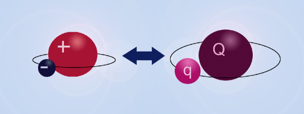
Figure 1: The similarity between the hydrogen atom (left) and heavy meson (right).

The bilocal operator interpolating the heavy meson in the valence quark-antiquark approximation (the lowest Fock state) in the HQS limit is as follows [9]:

$$\widetilde{O}(z)=Q^{*}(0)\,{\cal P}\exp\left\{-ig_{\rm st}\int_{0}^{z}dz^{\prime\mu}A^{a}_{\mu}(z^{\prime})\,\frac{\lambda^{a}}{2}\right\}q(z)=Q^{*}(0)\,E(0,z)\,q(z).$$ (1)

The link between the quarks is the path-ordered exponential called the Wilson line [10], where $A^{a}_{\mu}(z)$ is the gluonic field, $g_{\rm st}$ is the strong coupling, and $\lambda^{a}$ ($a=1,\ldots,8$) are the Gell-Mann matrices. Sometimes it is convenient to use the notation: $A_{\mu}=A^{a}_{\mu}\lambda^{a}/2$.

In many exclusive decays of the $B$-meson only one projection of the light-quark momentum gives the dominant contribution into the decay amplitude. So, it is necessary to find such a direction and study the dependence of the meson quantities on the corresponding momentum projection. On this way, the light-cone representation of four-vectors appears to be very convenient. To get a corresponding decomposition, one needs to introduce a light cone and specify two light-like four-vectors on it, for example, $n_{\pm}^{\mu}=\left(1,0,0,\mp 1\right)/\sqrt{2}$, where $n_{\pm}^{2}=0$ and $(n_{+}n_{-})=1$. They can be related with physical vectors presented in a problem. In particular, if one assumes that the light quark in the bilocal operator (1) is a massless particle situated on the light cone and the gauge link is a straight line connecting its position with the origin, the four-vector $n_{+}^{\mu}$ can be directed along this link. In this case, $dz^{\prime\mu}=dz^{\prime}_{-}n_{+}^{\mu}$ in (1) and the variable $z^{\prime}_{-}$ specifies the position of the gluon field on the line. The decomposition of an arbitrary four-vector is as follows:

$$A^{\mu}=A_{+}n^{\mu}_{-}+A_{-}n^{\mu}_{+}+A_{\perp}^{\mu},$$ (2)

where $A_{\pm}=n^{\mu}_{\pm}A_{\mu}$ are two light-cone projections. Note that the scalar product $(A^{a}(z^{\prime})dz^{\prime})=A_{+}^{a}(z^{\prime}_{-})dz^{\prime}_{-}$ in the exponential in (1) and turns out to be zero in the Fock-Schwinger gauge $A_{+}^{a}(z^{\prime}_{-})=0$. In this gauge, adopted further in this paper, the gauge link becomes trivial, $E(0,z)=1$, and the expression for the meson bilocal current (1) simplifies.

The meson-to-vacuum transition matrix element at $z^{2}=0$ [9] is of our interest:

$$\langle 0|Q^{*}(0)\,q(z)|M(v)\rangle=f_{M}\left\{\tilde{\varphi}_{+}(t)+\left[\tilde{\varphi}_{-}(t)-\tilde{\varphi}_{+}(t)\right]\frac{\hat{z}}{2t}\right\}U(v),$$ (3)

where $f_{M}$ is a constant with the dimension of a mass, $t=(vz)$ is the time in the heavy-meson rest frame, where the meson four-velocity is $v^{\mu}=(1,0,0,0)$, the bispinor $U(v)$ is the non-relativistic wave-function of the “spinor-like” meson, and $\tilde{\varphi}_{\pm}(t)$ are the distribution amplitudes (DAs) of the heavy meson. The Fourier transforms of DAs are usually required in constructing matrix elements of heavy meson decays:

$$\tilde{\varphi}_{\pm}(t)=\int_{0}^{\infty}d\omega\,{\rm e}^{-i\omega t}\phi_{\pm}(\omega).$$ (4)

In performing calculations, it is convenient to introduce the projection operator onto the $B^{(*)}$-meson state. Note that the heavy $B$- and $B^{*}$-mesons are degenerate in this approach. The $B$-meson-to-vacuum transition matrix element at $z^{2}=0$ in the real world after the heavy-quark spin is taken into account can be written in the form [9, 11]:

$$\langle 0|\bar{q}_{\alpha}(z)\,h_{v,\beta}(0)|\bar{B}^{(*)}(v)\rangle=\eta_{B^{(*)}}\frac{if_{B^{(*)}}m_{B^{(*)}}}{4}\left[\left(1+\hat{v}\right)\left\{\tilde{\varphi}^{B}_{+}(t)-\left[\tilde{\varphi}^{B}_{+}(t)-\tilde{\varphi}^{B}_{-}(t)\right]\frac{\hat{z}}{2t}\right\}\gamma_{5}(\hat{\varepsilon})\right]_{\beta\alpha}\!\!\!,$$ (5)

where $\varepsilon^{\mu}$ is the polarization vector of the $B^{*}$-meson, $\eta_{B}=-1$ for the $B$-meson and $\eta_{B^{*}}=1$ for the $B^{*}$-meson. The HQS gives the relations $f_{B^{*}}=f_{B}$ and $\tilde{\varphi}^{B^{*}}_{\pm}(t)=\tilde{\varphi}^{B}_{\pm}(t)$.

The projection operator onto the three-particle state can be also determined through the $B$-meson-to-vacuum transition matrix element at $z^{2}=0$ both for the “spinor-like” meson and after the spin of the heavy quark is switched on. For this matrix element one needs to introduce four distribution amplitudes [12]: $\tilde{\Psi}_{A}^{B}(t,u)$, $\tilde{\Psi}_{V}^{B}(t,u)$, $\tilde{X}_{A}^{B}(t,u)$, and $\tilde{Y}_{A}^{B}(t,u)$. The corresponding projection operator $\langle 0|\bar{q}_{\alpha}(z)\,G_{\lambda\rho}(uz)\,h_{v,\beta}(0)|\bar{B}(v)\rangle$ was also worked out and can be found in [13]: A similar projection operator for $B^{*}$-meson-to-vacuum transition matrix element at $z^{2}=0$ can be easily obtained from the above one after making the replacement $\gamma_{5}\to\hat{\varepsilon}^{*}$ as in (5).

Equations of motion (EoM) for heavy and light quarks which are assumed to be on the mass shell result into relations among the $B$-meson DAs [12]:

$$\phi^{B}_{+}(\omega)+\omega\,\frac{d\phi^{B}_{-}(\omega)}{d\omega}=I(\omega),\quad\left(\omega-2\bar{\Lambda}\right)\phi^{B}_{+}(\omega)+\omega\,\phi^{B}_{-}(\omega)=J(\omega),$$ (6)

where $I(\omega)$ and $J(\omega)$ are determined by the three-particle quark-antiquark-gluon DAs [12]. The Wandzura-Wilczek [9] relation follows from the first equation in (6) when $I(\omega)=0$:

$$\phi^{B}_{-}(\omega)=\int_{\,\omega}^{\infty}\frac{\phi^{B}_{+}(\omega^{\prime})}{\omega^{\prime}}\,d\omega^{\prime}.$$ (7)

The basic property of the $B$-meson DAs is their scale dependence and one needs to know corresponding evolution equations. For the leading $B$-meson DA, this equation was worked out by B. Lange and M. Neubert [14]:

$$\frac{d\phi^{B}_{+}(\omega;\mu)}{d\ln\mu}=-\frac{\alpha_{\rm st}(\mu)\,C_{F}}{\pi}\int_{0}^{\infty}d\omega^{\prime}\,\gamma^{\rm LN}(\omega,\omega^{\prime};\mu)\,\phi^{B}_{+}(\omega^{\prime};\mu),$$ (8)

where $C_{F}=4/3$. The Lange-Neubert anomalous dimension is as follows [14]:

$$\gamma^{\rm LN}(\omega,\omega^{\prime};\mu)=\left(\ln\frac{\mu}{\omega}-\frac{5}{4}\right)\delta\left(\omega-\omega^{\prime}\right)-\Gamma_{\rm LN}(\omega^{\prime},\omega),$$ (9)

$$\Gamma_{\rm LN}(\omega^{\prime},\omega)=\left[\frac{\omega}{\omega^{\prime}}\,\frac{\Theta\left(\omega^{\prime}-\omega\right)}{\omega^{\prime}-\omega}+\frac{\Theta\left(\omega-\omega^{\prime}\right)}{\omega-\omega^{\prime}}\right]_{\oplus}.$$ (10)

Here, the $\oplus$-convention is introduced:

$$\int_{0}^{\infty}d\omega^{\prime}f(\omega^{\prime})\left[\gamma(\omega^{\prime},\omega)\right]_{\oplus}=\int_{0}^{\infty}d\omega^{\prime}\left[f(\omega^{\prime})-f(\omega)\right]\gamma(\omega^{\prime},\omega).$$ (11)

It was also shown in [14] that the Lange-Neubert kernel factorizes in the space of moments:

$$\tilde{\Gamma}_{\rm LN}(N)=\int_{0}^{\infty}d\omega\left(\frac{\omega}{\omega^{\prime}}\right)^{N-1}\Gamma_{\rm LN}(\omega^{\prime},\omega)=-\Psi(N)-\Psi(-N)-2\gamma_{\rm E},$$ (12)

where $\gamma_{\rm E}=0.577216$ is the Euler’s constant and $\Psi(x)=\Gamma^{\prime}(x)/\Gamma(x)$ is the digamma function. The analytic solution of the evolution equation can be written in the integral form as follows:

$$\phi^{B}_{+}(\omega;\mu)=\frac{1}{2\pi}\int_{-\infty}^{+\infty}dt\,\varphi_{0}(t)\,f(\omega,\mu,\mu_{0},it).$$ (13)

It depends on the function $f(\omega,\mu,\mu_{0},it)$ which can be calculated in the perturbation theory. The other function $\varphi_{0}(t)$ is arbitrary and fixed by the condition $\varphi_{0}(0)=\lambda_{B}^{-1}$ only. The shape of $\varphi_{0}(t)$ can be determined after a model for $\phi^{B}_{+}(\omega;\mu)$ is specified.

3 Applications of $B$-meson DAs

The $B$-meson distribution amplitudes, usually in the form of inverse moments, are entering the exclusive decay amplitudes of $B$-mesons. In this section some processes where the distribution amplitudes are important, are presented and briefly discussed.

3.1 $B^{+}\to\ell^{+}\nu_{\ell}\gamma$ Decay

Let us start the discussion with one of the most clean $B$-meson decay modes — the radiative leptonic $B^{+}\to\ell^{+}\nu_{\ell}\gamma$ decay. In the leading order in the perturbation theory, the decay amplitude is presented by two Feynman diagrams shown in Fig. 2 and can be written as follows:

$${\cal M}=\frac{4G_{F}}{\sqrt{2}}\,V_{ub}^{*}\left\langle\gamma(p,\epsilon)\left|\bar{b}\gamma_{\mu}\left(1-\gamma_{5}\right)u\right|B^{+}(v)\right\rangle\left[\bar{u}(q_{\ell})\gamma^{\mu}\left(1-\gamma_{5}\right)u(q_{\nu})\right].$$ (14)

Figure 2: The $B^{+}\to\ell^{+}\nu_{\ell}\gamma$ decay amplitudes in the leading order in perturbation theory.

The $B^{+}\to\gamma$ transition matrix element entering this amplitude can be parameterized by two form factors $F_{V}(E_{\gamma})$ and $F_{A}(E_{\gamma})$ [15]:

$$\left\langle\gamma(p,\epsilon)\left|\bar{b}(0)\gamma^{\mu}\left(1-\gamma_{5}\right)u(0)\right|B^{+}(v)\right\rangle$$ (15)

$$=\sqrt{4\pi\alpha}\left\{\varepsilon^{\mu\rho\sigma\tau}v_{\rho}p_{\sigma}\epsilon_{\tau}^{*}\,F_{V}(E_{\gamma})-i\left[(vp)\epsilon^{*\mu}-(v\epsilon^{*})p^{\mu}\right]F_{A}(E_{\gamma})\right\},$$

where $E_{\gamma}=(vp)=m_{B}\left(1-q^{2}/m_{B}^{2}\right)/2$ is the photon energy. The kinematical region of the process is determined by the condition $E_{\gamma}\gg\Lambda_{\rm QCD}$, with $\Lambda_{\rm QCD}$ being the QCD parameter, where perturbative QCD methods for exclusive processes can be applied.

It was demonstrated that in this order the factorization approach is applicable and the most convenient tool for the QCD factorization implementation is the Soft-Collinear Effective Theory (SCET) [16, 17, 18]. We are not going to discuss this theory in details but give the following references [19, 20], where a detail discussion of this theory can be found.

The differential width of the $B^{+}\to\ell^{+}\nu_{\ell}\gamma$ decay calculated within the SCET can be written in the form [21]:

$$\frac{d\Gamma}{dE_{\gamma}}=\frac{\alpha G_{F}^{2}f_{B}^{2}|V_{ub}|^{2}m_{B}^{4}}{54\pi^{2}}\,\left(C_{3}^{\rm SCET}\right)^{2}\frac{x_{\gamma}\left(1-x_{\gamma}\right)}{\Lambda_{B}^{2}(E_{\gamma})},$$ (16)

where $x_{\gamma}=2E_{\gamma}/m_{B}$ is the reduced photon energy. The coefficient $C_{3}^{\rm SCET}$ results after matching QCD and SCET operators at the hard scale $\mu_{F}=m_{B}$:

$$C_{3}^{\rm SCET}=1+\frac{\alpha_{s}(m_{B})C_{F}}{4\pi}\left[-2\log^{2}x_{\gamma}-2\,{\rm Li}_{2}(1-x_{\gamma})+\frac{3x_{\gamma}-2}{x_{\gamma}-1}\log x_{\gamma}-6-\frac{\pi^{2}}{12}\right].$$ (17)

The differential decay width (16) depends on non-perturbative parameters — the first inverse moment of the leading DA $\phi^{B}_{+}(k_{+};\mu_{F})$ and its logarithmic extensions in the form [21]:

$$\Lambda_{B}^{-1}(E_{\gamma})=e^{-S(E_{\gamma};\mu_{F})}\int\frac{dk_{+}}{k_{+}}\,\phi^{B}_{+}(k_{+};\mu_{F})\left\{1+\frac{\alpha_{s}C_{F}}{4\pi}\left[\log^{2}\frac{2E_{\gamma}k_{+}}{\mu_{F}^{2}}-\frac{\pi^{2}}{12}-1\right]\right\}.$$ (18)

Here, the exponential factor $e^{-S(E_{\gamma};\mu_{F})}$ appears after resummation of large Sudakov logarithms. It should be noted that power corrections of order of ${\cal O}(1/m_{B},1/(2E_{\gamma}))$ to the decay rate are also calculated recently [22].

The $B^{+}\to\ell^{+}\nu_{\ell}\gamma$ decay was a subject of intensive experimental searches on the $B$-factories at SLAC and KEK. In particular, the experimental analysis for the partial branching fraction in the photon-energy interval $E_{\gamma}^{\rm sig}=[1~{}{\rm GeV},m_{B}/2]$ with the full dataset of $(771.6\pm 10.6)\times 10^{6}$ $B\bar{B}$ pairs has been reported by the Belle collaboration recently [23]. The upper limits ($@\,90\%$ C. L.) presented are as follows: ${\cal B}(B^{+}\to e^{+}\nu_{e}\gamma)<6.1\times 10^{-6}$, ${\cal B}(B^{+}\to\mu^{+}\nu_{\mu}\gamma)<3.4\times 10^{-6}$, and ${\cal B}(B^{+}\to\ell^{+}\nu_{\ell}\gamma)<3.5\times 10^{-6}$. The last one was translated into the restriction on the first inverse moment [23]:

$$\lambda_{B}=\left[\int_{0}^{\infty}\frac{dk_{+}}{k_{+}}\,\phi^{B}_{+}(k_{+})\right]^{-1}>238~{}{\rm MeV}.$$ (19)

This result is in good agreement with the theoretical estimates being within the interval : $300~{}{\rm MeV}<\lambda_{B}<600~{}{\rm MeV}$.

The related topic is the shape of the $B^{+}\to\gamma$ form factors entering the transition matrix element (15). Both the vector and axial-vector form factors with account of the soft contribution are known [24]. Neglecting radiative and $1/m_{B}$ corrections, the form factors are equal $F_{V}^{(0)}=F_{A}^{(0)}=F_{B\to\gamma^{*}}^{(0)}$. The corresponding soft contribution is estimated by the LCSRs method [24]:

$$F_{B\to\gamma^{*}}^{(0)}(E_{\gamma})=\frac{Q_{u}f_{B}m_{B}}{2E_{\gamma}\lambda_{B}(\mu)}+\frac{Q_{u}f_{B}m_{B}}{2E_{\gamma}}\int_{0}^{\omega_{0}}d\omega\left[\frac{2E_{\gamma}}{m_{\rho}^{2}}\,e^{-(2E_{\gamma}\omega-m_{\rho}^{2})/M^{2}}-\frac{1}{\omega}\right]\phi^{B}_{+}(\omega,\mu),$$ (20)

where $Q_{u}=2/3$ is the electric charge of the $u$-quark, $M$ is the Borel parameter, and $m_{\rho}\simeq 775$ MeV is the $\rho$-meson mass [8]. Note that the isospin symmetry is implicitly assumed which means that the difference between the $\rho$- and $\omega$-mesons is neglected. The soft part of the form factor (the second term in (20)) is also dependent on the other non-perturbative parameter — the effective threshold $s_{0}=1.2$ GeV, where $\omega_{0}=s_{0}/(2E_{\gamma})$. It was also demonstrated that a choice of a model for the $B$-meson DA influences a result for the form factor but this dependence is not substantial.

3.2 $B_{q}\to\gamma\gamma$ and $B_{q}\to\ell^{+}\ell^{-}\gamma$ Decays

The interesting problem within the SCET is the universality of non-perturbative effects in leptonic and radiative $B$-meson decays. Let us start with the radiative $B_{q}\to\gamma\gamma$ decay, where $q=d$ or $s$, the decay width of which can be written as follows [25]:

$$\Gamma=\frac{\alpha^{2}G_{F}^{2}f_{B}^{2}m_{B}^{5}}{144\pi^{3}}\,|V_{tq}V_{tb}^{*}|^{2}\left|C_{7}^{\rm eff}C_{9}^{\rm SCET}\right|^{2}\frac{1}{\Lambda_{B}^{2}(m_{B}/2)}.$$ (21)

Similar processes are the ones where one of the photons is virtual and decaying into the lepton pair. The differential decay width of $B_{q}\to\ell^{+}\ell^{-}\gamma$, where $\ell=e,\,\mu$, has the form [25]:

$$\frac{d\Gamma}{dE_{\gamma}}=\frac{\alpha^{3}G_{F}^{2}f_{B}^{2}m_{B}^{4}}{1728\pi^{4}}\,|V_{tq}V_{tb}^{*}|^{2}\frac{x_{\gamma}\left(1-x_{\gamma}\right)}{\Lambda_{B}^{2}(E_{\gamma})}\left[\left|C_{9}^{\rm eff}C_{3}^{\rm SCET}+\frac{2C_{7}^{\rm eff}}{1-x_{\gamma}}\,C_{9}^{\rm SCET}\right|^{2}+\left|C_{10}C_{3}^{\rm SCET}\right|^{2}\right],$$ (22)

where $x_{\gamma}=2E_{\gamma}/m_{B}$. The coefficient $C_{3}^{\rm SCET}$ (17) determines the differential width of the $B^{+}\to\ell^{+}\nu_{\ell}\gamma$ decay while the decays considered above are dependent on the other coefficient $C_{9}^{\rm SCET}$ which also results after perturbative matching of QCD and SCET operators at the scale $\mu_{F}=m_{B}$:

$$C_{9}^{\rm SCET}=1+\frac{\alpha_{s}(m_{B})C_{F}}{4\pi}\left[\log\frac{m_{B}^{2}}{\mu_{R}}-2\log^{2}x_{\gamma}+2\log x_{\gamma}-2\,{\rm Li}_{2}(1-x_{\gamma})-6-\frac{\pi^{2}}{12}\right].$$ (23)

These examples explicitly show the necessity to know two coefficients $C_{3}^{\rm SCET}$ and $C_{9}^{\rm SCET}$ only for performing theoretical analysis of the radiative and leptonic radiative $B$-mesons decays. As for the $B$-meson DAs, all three decays considered are dependent on $\Lambda_{B}^{-1}(\mu)$ (18) and this quantity can be independently determined from the analysis of each decay. This can be a good universality test of the soft contribution determined by the $B$-meson dynamics.

3.3 $B^{+}\to\pi^{+}\ell^{+}\ell^{-}$ Decays

The other good example of the $B$-meson decays which are sensitive to the $B$-meson distribution amplitudes are rare semileptonic decays like the $B^{+}\to P\,\ell^{+}\ell^{-}$ decay, where $P=\pi,\,K,\,\eta^{(\prime)}$ and $\ell=e,\,\mu$. In this lecture some details of the $B^{+}\to\pi^{+}\ell^{+}\ell^{-}$ decay are presented.

Detailed perturbative analysis in full kinematical region of $q^{2}$, the lepton-pair invariant mass squared, was undertaken in [26]. The differential branching fraction is as follows:

$$\frac{d\mbox{Br}\left(B^{+}\to\pi^{+}\ell^{+}\ell^{-}\right)}{dq^{2}}=\frac{G_{F}^{2}\alpha_{\rm em}^{2}\tau_{B}}{1024\pi^{5}m_{B}^{3}}|V_{tb}V_{td}^{*}|^{2}\sqrt{\lambda(q^{2})}\sqrt{1-\frac{4m_{\ell}^{2}}{q^{2}}}F(q^{2}).$$ (24)

This expression contains the dynamical function:

$$F(q^{2}) = \frac{2}{3}\,\lambda(q^{2})\left(1+\frac{2m_{\ell}^{2}}{q^{2}}\right)\left|C_{9}^{\rm eff}f_{+}(q^{2})+\frac{2m_{b}}{m_{B}+m_{\pi}}\,C_{7}^{\rm eff}f_{T}(q^{2})\right|^{2}$$

$$+ \frac{2}{3}\,\lambda(q^{2})\left(1-\frac{4m_{\ell}^{2}}{q^{2}}\right)\left|C_{10}^{\rm eff}\right|^{2}f_{+}^{2}(q^{2})+\frac{4m_{\ell}^{2}}{q^{2}}\left(m_{B}^{2}-m_{\pi}^{2}\right)^{2}\left|C_{10}^{\rm eff}\right|^{2}f_{0}^{2}(q^{2}),$$

where $C_{i}^{\rm eff}$ are the effective Wilson coefficients which are specific combinations of Wilson coefficients entering the effective weak $b\to d$ Hamiltonian:

$${\cal H}_{\rm eff}^{(b\to d)}=-\frac{4G_{F}}{\sqrt{2}}\!\biggl{[}V_{tb}^{*}V_{td}\sum\limits_{i=1}^{10}\!C_{i}(\mu){\cal O}_{i}(\mu)+V_{ub}^{*}V_{ud}\sum\limits_{i=1}^{2}\!C_{i}(\mu)\!\left(\!{\cal O}_{i}(\mu)-{\cal O}_{i}^{(u)}(\mu)\!\right)\!\biggr{]}+{\rm h.\,c.}$$ (26)

Here, $G_{F}$ is the Fermi constant, $C_{i}(\mu)$ are Wilson coefficients, ${\cal O}_{i}(\mu)$ are the dimension-six operators, and $V_{ij}$ are Cabibbo-Kobayashi-Maskawa (CKM) matrix elements. One can easily recognize that the products $V_{tb}^{*}V_{td}\sim V_{ub}^{*}V_{ud}\sim\lambda^{3}$ are of the same order in $\lambda=\sin\theta_{C}$, where $\theta_{C}$ is the Cabibbo angle.

The dynamical function (3.3) is depended on three form factors $f_{+}(q^{2})$, $f_{0}(q^{2})$, and $f_{T}(q^{2})$ which are non-perturbative scalar functions of the momentum transfered squared. They are entering the vector and tensor $B\to\pi$ transition matrix elements. The Heavy-Quark Symmetry (HQS) is applicable in the large-recoil limit (small $q^{2}$-values) and relates these form factors [11]:

$$f_{0}(q^{2}) = \left(\frac{m_{B}^{2}+m_{\pi}^{2}-q^{2}}{m_{B}^{2}}\right)\Biggl{[}\left\{1+\frac{\alpha_{s}(\mu)C_{F}}{4\pi}\left(2-2L(q^{2})\right)\right\}f_{+}(q^{2})$$ (27)

$$+ \frac{\alpha_{s}(\mu)C_{F}}{4\pi}\frac{m_{B}^{2}(q^{2}-m_{\pi}^{2})}{(m_{B}^{2}+m_{\pi}^{2}-q^{2})^{2}}\Delta F_{\pi}\Biggr{]},$$

$$f_{T}(q^{2}) = \left(\frac{m_{B}+m_{\pi}}{m_{B}}\right)\Biggl{[}\left(1+\frac{\alpha_{s}(\mu)C_{F}}{4\pi}\left(\ln\frac{m_{b}^{2}}{\mu^{2}}+2L(q^{2})\right)\right)f_{+}(q^{2})$$ (28)

$$- \frac{\alpha_{s}(\mu)C_{F}}{4\pi}\frac{m_{B}^{2}}{m_{B}^{2}+m_{\pi}^{2}-q^{2}}\Delta F_{\pi}\Biggr{]},$$

where for simplicity the following quantities are introduced:

$$L(q^{2})=\left(1+\frac{m_{B}^{2}}{m_{\pi}^{2}-q^{2}}\right)\ln\!\left(1+\frac{m_{\pi}^{2}-q^{2}}{m_{B}^{2}}\right),\qquad\Delta F_{\pi}=\frac{8\pi^{2}f_{B}f_{\pi}}{N_{c}m_{B}\lambda_{B}}\left<\bar{u}^{-1}\right>_{\pi}.$$ (29)

The last quantity $\Delta F_{\pi}$ contains the first inverse moments of $\pi$- and $B$-meson:

$$\left<\bar{u}^{-1}\right>_{\pi}=\int\!du\frac{\phi_{\pi}(u)}{1-u},\qquad\lambda_{B}^{-1}\equiv\left<\bar{\omega}^{-1}\right>_{+}=\int\!d\omega\frac{\phi^{B}_{+}(\omega)}{\omega}.$$ (30)

Only one form factor $f_{+}(q^{2})$ is required for getting the $q^{2}$-distribution in this decay which can be fitted from the data on the $B\to\pi\ell^{+}\nu_{\ell}$ decays [26].

Within the factorization approach, it is also possible to calculate some types of power-suppressed corrections in the $B\to\pi\ell^{+}\ell^{-}$ decay, in particular, the annihilation contributions. This type of corrections contains the $q^{2}$-dependent first inverse moment of the sub-leading $B$-meson LCDA:

$$\lambda_{B,-}^{-1}(q^{2})=\int_{0}^{\infty}\!\!\frac{\phi^{B}_{-}(\omega)\,d\omega}{\omega-q^{2}/M_{B}-i\epsilon}.$$ (31)

Note the specific feature of this moment: it is logarithmically divergent at $q^{2}\to 0$ because the sub-leading LCDA $\phi^{B}_{-}(\omega)$ turns out to be constant at small $\omega$, $\phi^{B}_{-}(\omega)|_{\omega\to 0}\sim{\rm const}$. Nevertheless, such a fiture does not result a problem in the numerical analysis of the differential branching fraction as the kinematical lower cut $q^{2}\geq 4m_{\ell}^{2}$ exists in the semileptonic $B\to\pi\ell^{+}\ell^{-}$ decay. Annihilation contributions of a similar type enter also in decay amplitudes of similar semileptonic $B\to V_{\|}\ell^{+}\ell^{-}$ decays, where $V_{\|}$ is the longitudinally polarized light vector meson [27]. Decays with a transversely polarized vector meson in the final state are dependent on $\phi^{B}_{+}(\omega)$ to the leading order. In the limit $q^{2}=0$, the corresponding branching fraction is finite and can be related with the branching ratios of rare radiative $B\to V\gamma$ decays.

3.4 Models for the $B$-Meson Distribution Amplitudes

The distribution amplitudes are non-perturbative quantities and usual perturbative methods of QFT [10] are inapplicable. The commonly used method of their calculation is the QCD Sum Rules [9, 28]. To combine these distribution amplitudes with hard kernels in amplitudes of physical processes, one needs to model them by some analytical expressions called the distribution amplitude models. At present, several models for the distribution amplitudes have been suggested. Two simplest ones are the exponential models [9]:

$$\phi^{+}_{B}(\omega)=\frac{\omega}{\omega_{0}^{2}}\,e^{-\omega/\omega_{0}},\qquad\phi^{-}_{B}(\omega)=\frac{1}{\omega_{0}}\,e^{-\omega/\omega_{0}},$$ (32)

where $\omega_{0}=2\bar{\Lambda}/3$, which appeared to be the most popular in physical applications, and the light-meson-like models [12]:

$$\phi^{+}_{B}(\omega)=\frac{\omega}{2\bar{\Lambda}^{2}}\,\theta(2\bar{\Lambda}-\omega),\qquad\phi^{-}_{B}(\omega)=\frac{2\bar{\Lambda}-\omega}{2\bar{\Lambda}^{2}}\,\theta(2\bar{\Lambda}-\omega),$$ (33)

which is also simple and explicitly based on the light-meson distribution amplitude. The energy dependence of these distribution amplitudes is presented in Fig. 3.

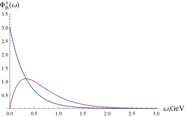
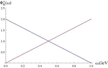
Figure 3: The energy dependence of of both leading and non-leading distribution amplitude models where the exponential ones are presented on the left panel and the light-meson-like models are on the right panel.

More involved models are the two-parametric model by Braun, Ivanov, and Korchemsky (BIK) [28] and improved exponential model by Lee and Neubert [29]. The later one matches the exponential behavior at low momenta of light quark and QCD-based behavior (the radiative tail) at large momenta. For these models the leading distribution amplitude only was studied while the non-leading amplitude was skipped.

As mentioned above, one needs moments of these amplitudes in getting decay widths of heavy mesons. Among moments, first inverse ones are of special interest. The uncertainty induced by a choice of the distribution amplitude model of the heavy meson on the semileptonic decay rates of $B$-mesons is also interesting to study which is not yet been worked out.

4 Light-Cone Distribution Amplitudes of Heavy Baryons

Light-cone distribution amplitudes (LCDAs) of heavy baryons are the transition matrix elements from the baryonic state to vacuum of non-local light-ray operators built off an effective heavy quark and two light quarks. The content of such operators supports a similarity in the construction of the heavy-baryon LCDAs to both the $B$-meson (within the HQET) [9, 28] and the nucleon (within QCD) [30, 31] LCDAs descriptions. An important simplifying feature of the operators containing one or more heavy quarks is an existence of the Heavy Quark Symmetry (HQS) which results into the decoupling of the heavy-quark spin from the system dynamics in the limit $m_{Q}\to\infty$, where $m_{Q}$ is the heavy-quark mass. So, to understand the properties of heavy baryons in this limit, it is enough to switch off the heavy-quark spin and to introduce a total set of two-particle LCDAs corresponding to the light-quark system, called diquark, which quantum numbers completely determine a number of LCDAs and their asymptotic behavior.

In this simplified picture, there are the $SU(3)_{F}$ antitriplet of “scalar baryons” with the $J^{P}=0^{+}$ spin-parity determined by the diquark spin-parity $j^{p}=0^{+}$ and the $SU(3)_{F}$ sextet of “axial-vector baryons” with the $J^{P}=1^{+}$ spin-parity which follows from the diquark spin-parity $j^{p}=1^{+}$. It is reasonable to start with the description of the “scalar baryons” and then to generalize the procedure on the “axial-vector baryons”. The changes originated by an account of the heavy-quark spin can be done after the total sets of the non-local operators and corresponding LCDAs are introduced in the decoupling limit. All these steps are discussed briefly in this section.

4.1 “Scalar Baryons”

The “scalar baryons” are combined into the $SU(3)_{F}$ antitriplet with $J^{P}=0^{+}$ in which the light diquark states are also the scalar states with $j^{p}=0^{+}$.

The set of the LCDAs is determined by the matrix elements between the baryonic state and vacuum of the four independent non-local light-ray operators [32, 33, 34]:

$$\epsilon^{abc}\langle 0|\left(q_{1}^{a}(t_{1}n)C\gamma_{5}\hat{n}q_{2}^{b}(t_{2}n)\right)h^{c}_{v}(0)|H(v)\rangle = f^{(2)}_{H}\,\Psi_{2}(t_{1},t_{2}),$$ (34)

$$\epsilon^{abc}\langle 0|\left(q_{1}^{a}(t_{1}n)C\gamma_{5}q_{2}^{b}(t_{2}n)\right)h^{c}_{v}(0)|H(v)\rangle = f^{(1)}_{H}\,\Psi_{3}^{s}(t_{1},t_{2}),$$

$$\epsilon^{abc}\langle 0|\left(q_{1}^{a}(t_{1}n)C\gamma_{5}i\sigma_{\bar{n}n}q_{2}^{b}(t_{2}n)\right)h^{c}_{v}(0)|H(v)\rangle = 2f^{(1)}_{H}\,\Psi_{3}^{\sigma}(t_{1},t_{2}),$$

$$\epsilon^{abc}\langle 0|\left(q_{1}^{a}(t_{1}n)C\gamma_{5}\hat{\bar{n}}q_{2}^{b}(t_{2}n)\right)h^{c}_{v}(0)|H(v)\rangle = f^{(2)}_{H}\Psi_{4}(t_{1},t_{2}),$$

where $q_{i}(x)=u(x),\,d(x),\,s(x)$ are the light-quark fields, $h_{v}(0)$ is the static heavy-quark field situated at the origin of the position-space frame, $C$ is the charge conjugation matrix, $n^{\mu}$ and $\bar{n}^{\mu}$ are two light-like vectors normalized by the condition $(n\bar{n})=2$, and $\sigma_{\bar{n}n}=i\left(\hat{\bar{n}}\hat{n}-\hat{n}\hat{\bar{n}}\right)/2$. In addition, the frame is adopted where the heavy-meson velocity is related to the light-like vectors as follows: $v^{\mu}=\left(n^{\mu}+\bar{n}^{\mu}\right)/2$. The light-quark fields on the light cone are assumed to be multiplied by the Wilson lines:

$$q(tn)=\left[0,tn\right]q(tn)={\rm P}\exp\left\{-ig_{\rm st}t\int_{0}^{1}d\alpha n^{\mu}\,A_{\mu}(\alpha tn)\right\}q(tn)=\sum_{N=0}^{\infty}\frac{t^{N}}{N!}\,\left(n^{\mu}D_{\mu}\right)^{N}q(0),$$

where the following definition of the covariant derivative $D_{\mu}=\partial_{\mu}-ig_{\rm st}A_{\mu}$ is accepted. The static heavy-quark field living on the light cone also includes the Wilson line but of the other type with the time-like link [35]:

$$h_{v}(0)={\rm P}\exp\left\{ig_{\rm st}\int_{-\infty}^{0}d\alpha v^{\mu}\,A_{\mu}(\alpha v)\right\}\phi(-\infty),$$

with which it is connected with the sterile field $\phi(-\infty)$.

The couplings $f^{(i)}_{H}$ introduced in Eqs. (34) to make the LCDAs dimensionless are defined by local operators [36, 37, 38, 39]:

$$\epsilon^{abc}\langle 0|\left(q_{1}^{a}(0)C\gamma_{5}q_{2}^{b}(0)\right)h^{c}_{v}(0)|H(v)\rangle=f^{(1)}_{H},$$

$$\epsilon^{abc}\langle 0|\left(q_{1}^{a}(0)C\gamma_{5}\hat{v}q_{2}^{b}(0)\right)h^{c}_{v}(0)|H(v)\rangle=f^{(2)}_{H}.$$

The scale dependences of these couplings are governed by the anomalous dimensions $\gamma^{(i)}$ of local operators as follows:

$$\frac{d\ln f_{H}^{(i)}(\mu)}{d\ln\mu}\equiv-\gamma^{(i)}=-\sum_{k}\gamma^{(i)}_{k}\,a^{k}(\mu),\qquad a(\mu)\equiv\frac{\alpha_{s}^{\overline{\rm MS}}(\mu)}{4\pi},$$

where the strong coupling is determined in the $\overline{\rm MS}$-scheme. This equation can be solved order by order in the $a(\mu)$-power expansion and in the NLO order, one can use the following formula:

$$f^{(i)}_{H}(\mu)=f^{(i)}_{H}(\mu_{0})\left(\frac{\alpha_{s}(\mu)}{\alpha_{s}(\mu_{0})}\right)^{\gamma^{(i)}_{1}/\beta_{0}}\left[1-\frac{\alpha_{s}(\mu_{0})-\alpha_{s}(\mu)}{4\pi}\,\frac{\gamma^{(i)}_{1}}{\beta_{0}}\left(\frac{\gamma^{(i)}_{2}}{\gamma^{(i)}_{1}}-\frac{\beta_{1}}{\beta_{0}}\right)\right],$$

where $\beta_{0,1}$ are the first two coefficient in the perturbative expansion of the $\beta$-function. As the evolution to the required scale can be easily done now, one needs to know numerical values of the couplings $f^{(i)}_{H}(\mu)$ at some representative scale $\mu_{0}$, say $\mu_{0}=1$ GeV. As this scale is rather low to use the perturbation theory, non-perturbative techniques are necessary to calculate the value. In particular, the QCD sum rules method in NLO for the $\Lambda_{b}$-baryon results [39]:

$$f^{(1)}_{\Lambda_{b}}(\mu_{0}=1~{}{\rm GeV})\simeq f^{(2)}_{\Lambda_{b}}(\mu_{0}=1~{}{\rm GeV})\simeq 0.030\pm 0.005~{}\mbox{\rm GeV}^{3}.$$

Non-relativistic constituent-quark picture of heavy baryons $H$ suggests that $f^{(2)}_{H}\simeq f^{(1)}_{H}$ at low scales of order 1 GeV, and this expectation is supported by numerous QCD sum rule calculations [37, 36, 38, 39]. These couplings $f^{(i)}_{H}(\mu)$ cannot coincide at all scales because of different anomalous dimensions $\gamma^{(i)}$ of local operators.

Similar to the couplings $f^{(i)}_{H}(\mu)$, the LCDAs $\Psi_{i}(t_{1},t_{2})$ introduced in Eq. (34) are also scale-dependent functions. To find their scale evolution, it is convenient to make their Fourier transform to the momentum space:

$$\Psi(t_{1},t_{2})=\int_{0}^{\infty}\!\!d\omega_{1}\int_{0}^{\infty}\!\!d\omega_{2}\,e^{-it_{1}\omega_{1}-it_{2}\omega_{2}}\psi(\omega_{1},\omega_{2})=\int_{0}^{\infty}\!\!\omega\,d\omega\int_{0}^{1}du\,e^{-i\omega(t_{1}u+t_{2}\bar{u})}\,\widetilde{\psi}(\omega,u),$$

where $\bar{u}=1-u$. In the first representation $\omega_{1}=u\omega$ and $\omega_{2}=\left(1-u\right)\omega=\bar{u}\omega$ are the energies of the light quarks $q_{1}$ and $q_{2}$. The leading-order evolution equation for $\psi_{2}(\omega_{1},\omega_{2};\mu)$ can be derived by identifying the ultra-violet singularities of the one-gluon-exchange diagrams [32]. The evolution equation in the leading order is expressed in terms of two-particle kernels:

$$\mu\frac{d}{d\mu}\,\psi_{2}(\omega_{1},\omega_{2};\mu)=-\frac{\alpha_{s}(\mu)}{2\pi}\,\frac{4}{3}\,\Bigg{\{}\int_{0}^{\infty}d\omega_{1}^{\prime}\,\gamma^{\rm LN}(\omega_{1}^{\prime},\omega_{1};\mu)\,\psi_{2}(\omega^{\prime}_{1},\omega_{2};\mu)$$

$$\hskip 8.53581pt+\int_{0}^{\infty}d\omega_{2}^{\prime}\,\gamma^{\rm LN}(\omega_{2}^{\prime},\omega_{2};\mu)\,\psi_{2}(\omega_{1},\omega^{\prime}_{2};\mu)-\int_{0}^{1}dv\,V(u,v)\,\psi_{2}(v\omega,\bar{v}\omega;\mu)+\frac{3}{2}\,\psi_{2}(\omega_{1},\omega_{2};\mu)\Bigg{\}},$$

where the kernel $\gamma^{\rm LN}(\omega^{\prime},\omega;\mu)$ controls the evolution of the $B$-meson LCDA [14] and $V(u,v)$ is the Efremov-Radyushkin-Brodsky-Lepage (ER-BL) kernel [40, 41]. The term $3\psi_{2}(\omega_{1},\omega_{2};\mu)/2$ results from the one-loop $f^{(2)}_{H}$ renormalization subtraction. The evolution equation above can be solved either numerically or semi-analytically [32, 34].

The next step in working out solutions of the heavy-baryon evolution equations analytically was undertaken in [42]. In particular, the eigenfunctions of the Lange-Neubert evolution kernel were found and used for a systematic implementation of the renormalization-group effects for both the $B$-meson and $\Lambda_{b}$-baryon wave-function evolutions. Based on these foundations, the new strategy to construct the LCDA models in accordance with the Wandzura-Wilczek-like relations was presented. As a possible extension of the above analysis in application to baryons, the classification of the non-local baryonic operators constructed from four particles (three quarks and a gluon) is required to work out equations involving explicitly the there-particle LCDAs and twist-four four-particle ones which should reduce to the Wandzura-Wilczek relations after four-particle LCDAs are neglected.

4.2 “Axial-Vector Baryons”

The “axial-vector baryons” are components of the $SU(3)_{F}$ sextet with $J^{P}=1^{+}$ in which the light diquark states are the axial-vector states with $j^{p}=1^{+}$. In a difference to the “scalar baryons” case, one needs to consider the baryons with the longitudinal and transverse polarizations separately.

The set of the longitudinal LCDAs is determined by the matrix elements between the baryonic state with the appropriate polarization and vacuum of the four independent non-local light-ray operators [33, 34]:

$$\epsilon^{abc}\langle 0|\left(q_{1}^{a}(t_{1})C\,\hat{n}q_{2}^{b}(t_{2})\right)h_{v}^{c}(0)|H(v,\varepsilon)\rangle = \left(\bar{v}\varepsilon\right)f^{(2)}_{H}\,\Psi_{2}^{\|}(t_{1},t_{2})$$

$$\epsilon^{abc}\langle 0|\left(q_{1}^{a}(t_{1})C\,q_{2}^{b}(t_{2})\right)h_{v}^{c}(0)|H(v,\varepsilon)\rangle = \left(\bar{v}\varepsilon\right)f^{(1)}_{H}\,\Psi_{3}^{\|s}(t_{1},t_{2})$$

$$\epsilon^{abc}\langle 0|\left(q_{1}^{a}(t_{1})C\,i\sigma_{\bar{n}n}q_{2}^{b}(t_{2})\right)h_{v}^{c}(0)|H(v,\varepsilon)\rangle = 2\left(\bar{v}\varepsilon\right)f^{(1)}_{H}\,\Psi_{3}^{\|a}(t_{1},t_{2})$$

$$\epsilon^{abc}\langle 0|\left(q_{1}^{a}(t_{1})C\,\hat{\bar{n}}q_{2}^{b}(t_{2})\right)h_{v}^{c}(0)|H(v,\varepsilon)\rangle = -\left(\bar{v}\varepsilon\right)f^{(2)}_{H}\,\Psi_{4}^{\|}(t_{1},t_{2})$$

where $\bar{v}^{\mu}=\left(\bar{n}^{\mu}-n^{\mu}\right)/2$ is the four-vector normalized as $(\bar{v}\bar{v})=-1$ and orthogonal to the four-velocity $(v\bar{v})=0$. In the LCDA definitions above, the baryonic state is assumed to have a pure longitudinal polarization $\varepsilon_{\|}^{\mu}=\bar{v}^{\mu}$ and the prefactor on the r.h.s. is simply $(\bar{v}\varepsilon)=-1$.

The similar set of the transverse LCDAs is determined as follows [33, 34]:

$$\epsilon^{abc}\langle 0|\left(q_{1}^{a}(t_{1})C\,\gamma_{\perp}^{\mu}\hat{n}q_{2}^{b}(t_{2})\right)h_{v}^{c}(0)|H(v,\varepsilon)\rangle = f^{(2)}_{H}\,\Psi_{2}^{\perp}(t_{1},t_{2})\,\varepsilon_{\perp}^{\mu}$$

$$\epsilon^{abc}\langle 0|\left(q_{1}^{a}(t_{1})C\,\gamma_{\perp}^{\mu}q_{2}^{b}(t_{2})\right)h_{v}^{c}(0)|H(v,\varepsilon)\rangle = f^{(1)}_{H}\,\Psi_{3}^{\perp s}(t_{1},t_{2})\,\varepsilon_{\perp}^{\mu}$$

$$\epsilon^{abc}\langle 0|\left(q_{1}^{a}(t_{1})C\,\gamma_{\perp}^{\mu}i\sigma_{\bar{n}n}q_{2}^{b}(t_{2})\right)h_{v}^{c}(0)|H(v,\varepsilon)\rangle = 2f^{(1)}_{H}\,\Psi_{3}^{\perp a}(t_{1},t_{2})\,\varepsilon_{\perp}^{\mu}$$

$$\epsilon^{abc}\langle 0|\left(q_{1}^{a}(t_{1})C\,\gamma_{\perp}^{\mu}\hat{\bar{n}}q_{2}^{b}(t_{2})\right)h_{v}^{c}(0)|H(v,\varepsilon)\rangle = f^{(2)}_{H}\,\Psi_{4}^{\perp}(t_{1},t_{2})\,\varepsilon_{\perp}^{\mu}$$

where $\gamma_{\perp}^{\mu}=\gamma^{\mu}-\left(\hat{\bar{n}}\hat{n}+\hat{n}\hat{\bar{n}}\right)/2$ and $\varepsilon_{\perp}^{\mu}=\varepsilon^{\mu}-\varepsilon_{\|}^{\mu}$ is the transverse polarization of the baryon.

4.3 Real Baryons

As far as all the sets of the LCDAs are determined, it necessary to generalize their definitions to real baryons which simply means that the spin of the heavy quark should be included into the baryon wave function. In other words, the r. h. s. of matrix elements of all non-local operators must be multiplied on the Dirac spinor $U(v)$ of the heavy quark $h_{v}$, satisfying the conditions: $\hat{v}\,U(v)=U(v)$ and $\overline{U}(v)\,U(v)=1$. After these modifications, the “scalar baryons” transform to the baryons with the spin-parity $J^{P}=1/2^{+}$ and the heavy-quark Dirac spinor $U(v)$ is nothing else but the heavy-baryon spinor $H(v)$, i. e. the spin of the heavy quark completely determines the spin structure of the heavy-baryon wave function. The case of “axial-vector baryons” is a little bit more complicated. It is well-known from quantum mechanics that the direct product of two angular momenta $j_{1}=1/2$ and $j_{2}=1$ is decomposed into two irreducible representations with the momenta $J_{1}=1/2$ and $J_{2}=3/2$. That is exactly the situation after the heavy-quark spin is switched on in the heavy baryon with the diquark in the axial-vector state $j^{p}=1^{+}$:

$$\varepsilon_{\mu}\,U(v)=\left[\varepsilon_{\mu}\,U(v)-\frac{1}{3}\left(\gamma_{\mu}+v_{\mu}\right)\hat{\varepsilon}\,U(v)\right]+\frac{1}{3}\left(\gamma_{\mu}+v_{\mu}\right)\hat{\varepsilon}\,U(v)\equiv R^{3/2}_{\mu}(v)+\frac{1}{3}\left(\gamma_{\mu}+v_{\mu}\right)H(v).$$

As the result, there are two states with the spin-parities $J^{P}=1/2^{+}$ and $J^{P}=3/2^{+}$. The former one is described by the Dirac spinor $H(v)$ and for the $J^{P}=3/2^{+}$ state the Rarita-Schwinger vector-spinor $R^{3/2}_{\mu}(v)$, which satisfies the relations $\hat{v}\,R^{3/2}_{\mu}(v)=R^{3/2}_{\mu}(v)$, $v^{\mu}\,R^{3/2}_{\mu}(v)=0$, and $\gamma^{\mu}\,R^{3/2}_{\mu}(v)=0$, is introduced.

4.4 QCD Sum Rules

In applications to a calculation of amplitudes with heavy baryons, one needs to know realistic models for LCDAs. Such models can be obtained by matching several few moments of LCDA models and the corresponding ones calculated by some non-perturbative methods, say by the QCD sum rules. The later method requires a calculation of a two-point correlator which involve the non-local light-ray operator and a suitable local current $J^{\Gamma^{\prime}}(x)$. The general structure of the heavy-baryon local current can be chosen as follows:

$$\bar{J}^{\Gamma^{\prime}}(x)=\epsilon^{abc}\left(\bar{q}_{2}^{a}(x)\left[A+B\,\hat{v}\right]\Gamma^{\prime}C^{T}\bar{q}_{1}^{b}(x)\right)\bar{h}_{v}^{c}(x),$$

where $A$ and $B$ are two constants satisfying the constraint $A+B=1$ which accounts for an arbitrariness in the choice of a local current. The variation in $A\in[0,1]$ is adopted as a systematic error of numerical estimations. Note that the central value $A=B=1/2$ corresponds to the constituent quark model picture [32]. The Dirac matrix $\Gamma^{\prime}$ is a suitable structure determined by the spin-parity of the baryon, in particular, $\Gamma^{\prime}=\gamma_{5}$ for baryons from the $SU(3)_{F}$ antitriplet ($j^{p}=0^{+}$) and $\Gamma^{\prime}=\gamma_{\|},\,\gamma_{\perp}$ for the $SU(3)_{F}$-sextet baryons with $j^{p}=1^{+}$.

In calculations of the correlation functions, one tacitly assumes that baryons are bound states of quarks which are not free particles inside but couple by virtue of the gluonic field. So, light quark propagators $\tilde{S}_{q}(x)$, being very sensitive to the influence of the background gluonic field, should be modified accordingly while for the heavy quark this effect is sub-dominant and to leading order in the heavy-quark mass $m_{Q}$ expansion can be neglected. To take effects of the QCD background inside baryons into account, the method of non-local condensates [43, 44, 45] is used. In this approach the light-quark propagator can be decomposed into two parts: the perturbative $S_{q}(x)$ and non-perturbative $\mathcal{C}_{q}(x)$ ones, and the later accumulates an information about the background inside the baryon in terms of non-local quark condensate $\langle\bar{q}(x)q(0)\rangle$.

To obtain the QCD sum rules, it is convenient to make the double Fourier transform of the correlation function:

$$\Pi_{\Gamma\Gamma^{\prime}}(\omega_{1},\omega_{2};E)=i\int_{-\infty}^{\infty}\frac{dt_{1}\,dt_{2}}{(2\pi)^{2}}\,e^{i(\omega_{1}t_{1}+\omega_{2}t_{2})}\int d^{4}x\,e^{-iE(vx)}\,\langle 0|{\cal O}^{\Gamma}(t_{1},t_{2})\,\bar{J}^{\Gamma^{\prime}}(x)|0\rangle$$

As it is well-known from the QCD-SR analysis within the HQET, the heavy-quark condensate term is suppressed by $1/m_{Q}$ and absent in the Heavy-Quark Symmetry limit. So, the QCD Sum Rules can be read off after the phenomenological and perturbatively calculated considerations of the correlation function are equated based on the idea of the quark-hadron duality [46]:

$$|f_{H}|^{2}\,\psi^{\Gamma}(\omega,u)\,e^{-\bar{\Lambda}_{H}/\tau}=\mathds{B}[\Pi](\omega,u;\tau,s_{0}),$$

where symbol $\mathds{B}$ means the Borel-transform, $\bar{\Lambda}_{H}=m_{H}-m_{Q}$ is the effective baryon mass in the HQET, and $s_{0}$ is the momentum cutoff resulting from applying the quark-hadron duality. The explicit QCD-SRs for all the baryonic non-local operators can be found in [34].

The numerical values of first several moments of the bottom-baryon LCDAs estimated by the QCD-SRs are presented in [34]. These moments should be matched to the corresponding moments of the model functions for the LCDAs. The general presentation of the model functions for the $b$-baryon LCDAs is governed by their scale evolution and can be composed of the exponential part corresponding to the heavy-light interaction and the Gegenbauer polynomials to the light-light interaction. The order of the polynomials is determined by the twist of the diquark system. Motivated by the analysis done for the $\Lambda_{b}$-baryon [32], the following simple models for the LCDAs have proposed [33, 34]:

$$\tilde{\psi}_{2}(\omega,u) = \omega^{2}u(1-u)\,\sum_{n=0}^{2}\frac{a^{(2)}_{n}}{{\epsilon^{(2)}_{n}}^{4}}\,C^{3/2}_{n}(2u-1)\,{\rm e}^{-\omega/\epsilon^{(2)}_{n}},$$

$$\tilde{\psi}_{3s}(\omega,u) = \frac{\omega}{2}\,\sum_{n=0}^{2}\frac{a^{(3)}_{n}}{{\epsilon^{(3)}_{n}}^{3}}\,C^{1/2}_{n}(2u-1)\,{\rm e}^{-\omega/\epsilon^{(3)}_{n}},$$

$$\tilde{\psi}_{3\sigma}(\omega,u) = \frac{\omega}{2}\,\sum_{n=0}^{3}\frac{b^{(3)}_{n}}{{\eta^{(3)}_{n}}^{3}}\,C^{1/2}_{n}(2u-1)\,{\rm e}^{-\omega/\eta^{(3)}_{n}},$$

$$\tilde{\psi}_{4}(\omega,u) = \sum_{n=0}^{2}\frac{a^{(4)}_{n}}{{\epsilon^{(4)}_{n}}^{2}}\,C^{1/2}_{n}(2u-1)\,{\rm e}^{-\omega/\epsilon^{(4)}_{n}}.$$

The qualitative behavior of the twist-2 LCDAs is presented in Fig. 4.

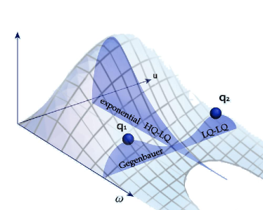
Figure 4: The general representation of the model functions for the heavy-baryon LCDAs with the $\omega$-dependence specific for the $B$-meson LCDAs and the $u$-dependence in terms of an expansion in the Gegenbauer polynomials similar to the ones for the light mesons.

The estimates of the parameters entering the theoretical models for the heavy-baryon LCDAs at the scale $\mu_{0}=1$ GeV can be found in [33, 34]. The $SU(3)_{F}$-symmetry breaking in LCDAs based on taking into account the $s$-quark difference from the $u$- and $d$-quarks is estimated to be approximately $15\%$ [33, 34].

5 Conclusions

A brief introduction into the heavy hadron wave-functions is given in the present lecture. The discussion is started from the simplest hadronic system — the heavy meson which is the bound state of the light quark and the heavy antiquark. An example of such a system are the $D$- and $B$-mesons which are containing the heavy $c$- and $b$-antiquarks, respectively. In the HQET, the dynamics in the heavy mesons is mainly determined by a motion of the light quark while the heavy antiquark can be considered as a static source. In many cases, not all the light-quark degrees of freedom are equally important and the dominant ones can be separated from the sub-dominant. Within this picture, it is possible to determine the so-called Light-Cone Distribution Amplitudes (LCDAs) of the heavy meson. Analysis shows that there are only two LCDAs in the lowest (two-particle) Fock decomposition and four more LCDAs in the three-particle heavy-meson state. The former two are mainly discussed in this lecture as well as their importance in calculations of branching fractions of radiative, leptonic and semileptonic $B$-meson decays. The last part is devoted to the bottom baryons which are the bound states of a heavy quark and two light ones. The total sets of the non-local light-ray operators for the ground-state heavy baryons with $J^{P}=1/2^{+}$ and $J^{P}=3/2^{+}$ are constructed in QCD in the heavy-quark limit. Matrix elements of these operators sandwiched between the heavy-baryon state and vacuum determine the LCDAs of different twist through the diquark current. Simple theoretical models for the LCDAs have been proposed and are briefly discussed. $SU(3)_{F}$ breaking effects result a correction of order 10%. Their application, for example, to transition matrix elements of heavy baryons is a good topic for future theoretical studies.

References

• [1] V. Khachatryan et al. [CMS and LHCb Collaborations], Nature 522, 68 (2015) [arXiv:1411.4413].
• [2] C. Bobeth et al., Phys. Rev. Lett.  112, 101801 (2014) [arXiv:1311.0903].
• [3] R. Aaij et al. [LHCb Collaboration], JHEP 1212, 125 (2012) [arXiv:1210.2645].
• [4] R. Aaij et al. [LHCb Collaboration], JHEP 1510, 034 (2015) [arXiv:1509.00414].
• [5] A. V. Manohar and M. B. Wise, “Heavy quark physics,” Camb. Monogr. Part. Phys. Nucl. Phys. Cosmol.  10, 1 (2000).
• [6] A. G. Grozin, “Heavy quark effective theory,” Springer Tracts Mod. Phys.  201, 1 (2004).
• [7] T. Mannel, “Effective Field Theories in Flavor Physics,” Springer Tracts Mod. Phys.  203, 1 (2004).
• [8] C. Patrignani et al. [Particle Data Group Collaboration], Chin. Phys. C 40, 100001 (2016).
• [9] A. G. Grozin and M. Neubert, Phys. Rev. D55, 272 (1997) [arXiv:hep-ph/9607366].
• [10] M. E. Peskin and D. V. Schroeder, “An Introduction to quantum field theory,” Reading, USA: Addison-Wesley (1995). 842 p.
• [11] M. Beneke and T. Feldmann, Nucl. Phys. B592, 3 (2001) [arXiv:hep-ph/0008255].
• [12] H. Kawamura, J. Kodaira, C. F. Qiao and K. Tanaka, Phys. Lett. B523, 111 (2001) [Erratum-ibid. B536, 344 (2002)] [arXiv:hep-ph/0109181].
• [13] A. Khodjamirian, T. Mannel and N. Offen, Phys. Rev. D75, 054013 (2007) [arXiv:hep-ph/0611193]
• [14] B. O. Lange and M. Neubert, Phys. Rev. Lett. 91 (2003) 102001 [arXiv:hep-ph/0303082].
• [15] G. P. Korchemsky, D. Pirjol, and T. M. Yan, Phys. Rev. D61, 114510 (2000) [arXiv:hep-ph/9911427].
• [16] C. W. Bauer, S. Fleming, D. Pirjol and I. W. Stewart, Phys. Rev. D63, 114020 (2001) [arXiv:hep-ph/0011336].
• [17] C. W. Bauer, D. Pirjol and I. W. Stewart, Phys. Rev. D65, 054022 (2002) [arXiv:hep-ph/0109045].
• [18] M. Beneke, A. P. Chapovsky, M. Diehl and T. Feldmann, Nucl. Phys. B643, 431 (2002) [arXiv:hep-ph/0206152].
• [19] T. Becher, A. Broggio and A. Ferroglia, Lect. Notes Phys.  896, pp. 1 (2015) [arXiv:1410.1892].
• [20] A. Grozin, arXiv:1611.08828 (this Proceedings).
• [21] S. Descotes-Genon and C. T. Sachrajda, Nucl. Phys. B650, 356 (2003) [arXiv:hep-ph/0209216].
• [22] M. Beneke and J. Rohrwild, Eur. Phys. J. C71, 1818 (2011) [arXiv:1110.3228].
• [23] A. Heller et al. [Belle Collaboration], Phys. Rev. D91, 112009 (2015) [arXiv:1504.05831].
• [24] V. M. Braun and A. Khodjamirian, Phys. Lett. B718, 1014 (2013) [arXiv:1210.4453].
• [25] S. Descotes-Genon and C. T. Sachrajda, Phys. Lett. B557, 213 (2003) [arXiv:hep-ph/0212162].
• [26] A. Ali, A. Y. Parkhomenko, and A. V. Rusov, Phys. Rev. D89, 094021 (2014) [arXiv:1312.2523].
• [27] M. Beneke, T. Feldmann and D. Seidel, Eur. Phys. J. C 41, 173 (2005) doi:10.1140/epjc/s2005-02181-5 [hep-ph/0412400].
• [28] V. M. Braun, D. Y. Ivanov and G. P. Korchemsky, Phys. Rev. D69, 034014 (2004) [arXiv:hep-ph/0309330].
• [29] S. J. Lee and M. Neubert, Phys. Rev. D 72, 094028 (2005) [arXiv:hep-ph/0509350].
• [30] V. M. Braun, S. E. Derkachov, G. P. Korchemsky and A. N. Manashov, Nucl. Phys. B553, 355 (1999) [arXiv:hep-ph/9902375].
• [31] V. Braun, R. J. Fries, N. Mahnke and E. Stein, Nucl. Phys. B589, 381 (2000) [Erratum-ibid. B607, 433 (2001)] [arXiv:hep-ph/0007279].
• [32] P. Ball, V. M. Braun and E. Gardi, Phys. Lett. B665, 197 (2008) [arXiv:0804.2424].
• [33] A. Ali, C. Hambrock, and A. Ya. Parkhomenko, Theor. Math. Phys. 170, 2 (2012) [Teor. Mat. Fiz. 170, 5 (2012)].
• [34] A. Ali, C. Hambrock, A. Ya. Parkhomenko, and W. Wang, Eur. Phys. J. C73, 2302 (2013) [arXiv:1212.3280].
• [35] G. P. Korchemsky and A. V. Radyushkin, Phys. Lett. B279, 359 (1992) [arXiv:hep-ph/9203222].
• [36] A. G. Grozin and O. I. Yakovlev, Phys. Lett. B285, 254 (1992) [arXiv:hep-ph/9908364].
• [37] E. Bagan, M. Chabab, H. G. Dosch and S. Narison, Phys. Lett. B301 (1993) 243.
• [38] S. Groote, J. G. Korner and O. I. Yakovlev, Phys. Rev. D55 (1997) 3016 [arXiv:hep-ph/9609469].
• [39] S. Groote, J. G. Korner and O. I. Yakovlev, Phys. Rev. D56, 3943 (1997) [arXiv:hep-ph/9705447].
• [40] A. V. Efremov and A. V. Radyushkin, Theor. Math. Phys. 42, 97 (1980) [Teor. Mat. Fiz. 42, 147 (1980)]; Phys. Lett. B94, 245 (1980).
• [41] G. P. Lepage and S. J. Brodsky, Phys. Lett. B87, 359 (1979); Phys. Rev. D22 (1980) 2157.
• [42] G. Bell, T. Feldmann, Y.-M. Wang and M. W. Y. Yip, JHEP 1311, 191 (2013) [arXiv:1308.6114].
• [43] S. V. Mikhailov and A. V. Radyushkin, JETP Lett. 43, 712 (1986) [Pisma Zh. Eksp. Teor. Fiz.  43, 551 (1986)].
• [44] S. V. Mikhailov and A. V. Radyushkin, Phys. Rev. D45, 1754 (1992).
• [45] A. P. Bakulev and S. V. Mikhailov, Phys. Rev. D65, 114511 (2002) [arXiv:hep-ph/0203046].
• [46] M. A. Shifman, A. I. Vainshtein and V. I. Zakharov, Nucl. Phys. B147, 385 (1979); Nucl. Phys. B147, 448 (1979).