Quantum Interval-Valued Probability: Contextuality and the Born Rule

Résumé

We present a mathematical framework based on quantum interval-valued probability measures to study the effect of experimental imperfections and finite precision measurements on defining aspects of quantum mechanics such as contextuality and the Born rule. While foundational results such as the Kochen-Specker and Gleason theorems are valid in the context of infinite precision, they fail to hold in general in a world with limited resources. Here we employ an interval-valued framework to establish bounds on the validity of those theorems in realistic experimental environments. In this way, not only can we quantify the idea of finite-precision measurement within our theory, but we can also suggest a possible resolution of the Meyer-Mermin debate on the impact of finite-precision measurement on the Kochen-Specker theorem.

I Introduction

In this investigation, we explore the implications of extending conventional quantum-mechanical probability measures to include the effect of imperfect measurements. There are long-standing debates in the foundations of quantum mechanics regarding the tension between finite precision measurement and contextuality Barrett and Kent (2004); Appleby (2005). The outcome of a theory that is contextual depends upon whether compatible sets of observables are measured together or separately; a non-contextual theory gives the same results in either case. A classic example of the varying opinions on the impact of imprecision is the claim by Meyer Meyer (1999) that finite-precision measurements invalidate the spirit of the Kochen-Specker theorem. This claim was countered in the same year by Havlicek et al. Havlicek et al. (1999) and Mermin Mermin (1999) and the debate continues to be an active topic of research Kent (1999); Simon et al. (2001); Cabello (2002); Larsson (2002); Appleby (2002); Barrett and Kent (2004); Appleby (2005); Spekkens (2005); Gühne et al. (2010); Mazurek et al. (2016).

The Kochen-Specker theorem Bell (1966); Kochen and Specker (1968); Redhead (1987); Mermin (1990); Peres (1995); Jaeger (2007); Held (2016) is in essence a mathematical statement about contextuality, asserting that in a Hilbert space of dimension $d\geq 3$, it is impossible to associate determinate probabilities, $\mu(P_{i})=0$ or $1$, with every projection operator $P_{i}$, in such a way that, if a set of commuting $P_{i}$ satisfies $\sum_{i}P_{i}=\mathbb{1}$, then $\sum_{i}\mu(P_{i})=1$. Meyer showed that one can assign determinate probabilities $0$ or $1$ to the measurement outcomes when the Hilbert space is defined over the field of rational numbers, therefore nullifying the theorem Meyer (1999). However, Mermin then argued that measurement outcomes must depend smoothly on slight changes in the experimental configuration, leading him to assert that the impact of Meyer’s negative result is “unsupportable” on physical grounds Mermin (1999). The question of how to address this controversy, and the effect of finite precision on measurements in general, is therefore a fundamental problem of physics. How does one develop mathematical theories of quantum mechanics that are intrinsically, rather than only implicitly, consistent with the resources available for the realistic accuracy of an actual measurement?

In this paper, we extend our previous work on the foundations of computability in quantum physics by exploring the application of interval-valued probability measures (IVPMs) to achieving a coherent formulation of finite-resource quantum mechanics. From this starting point, we develop a mathematical framework that includes the uncertainties of finite precision and imperfections in the quantum measurement process. In particular, we are able to suggest a way to quantify the concept of imperfect quantum measurement and its impact on the interpretation of the Kochen-Specker and Gleason theorems and their implications for the foundations of quantum mechanics. We have reason to believe that essential objectives of our program to achieve a computable theory of quantum mechanics and finite-resource measurement, attempted previously with computable number systems Willcock and Sabry (2011); Hanson et al. (2013, 2014), may be achievable by extending classical IVPMs Jamison and Lodwick (2004) to the quantum domain. We thus begin by axiomatizing a quantum interval-valued probability measure (QIVPM) framework.

To put our investigation in perspective, we note that Meyer attributes finite-precision errors exclusively to the description of the states defined in a general Hilbert space. Mermin’s response argues against Meyer’s interpretation but, indeed, accepts his framework. Others, however, have argued that the effect of finite-precision measurements on the Kochen-Specker theorem requires a different approach altogether (see for example Ax and Kochen’s communication cited by Cabello Cabello (2002)). Here, we propose such a new approach.

Our approach, based on QIVPMs, introduces the concept of $\delta$-determinism, where $\delta$ quantifies the effect of finite-precision uncertainties on measurement outcomes. Our parameter $\delta$ is not necessarily related to the description of states; we are agnostic about attributing elements of reality to the state function. Instead, we attribute lack of certainty to the uncertain results obtained through the use of a measuring instrument. Thus, the parameter $\delta$ in our framework reflects insufficient knowledge of the experimenter, which could be due to a variety of reasons related to imperfections of devices. For example, a typical question that an experimenter may not be able to answer accurately would be “did an electron land in the left half or the right half of the screen?” There are cases in which the electron would land too close to the middle of the screen for the experimenter to be able to determine with certainty that it was left or right of the center. We simply record this imprecision by generalizing the probabilities assigned to events to intervals reflecting the uncertainties.

We then recast the Kochen-Specker theorem using $\delta$-determinism to quantify the effects of finite precision and imperfections on contextuality. When $\delta=0$, the generalized theorem reduces to the conventional one, but as $\delta$ varies from 0 to 1 we note a transition from contextuality to non-contextuality. For a non-vanishing range of $\delta$, quantum-mechanical contextuality continues to hold, maintaining the Kochen-Specker result, but at a certain fixed value, $\delta=\frac{1}{3}$, there is a sharp transition to non-contextuality, parallel in spirit to a phase transition. These results provide a new insight into the Meyer-Mermin debate by presenting a theory in which there is a parameter interpolating between what appeared previously to be irreconcilable aspects of contextuality.

We also investigate the second key aspect of imprecise quantum measurement, which is its statistical nature as reflected in the application of the Born rule Born (1983); Mermin (2007); Jaeger (2007) determining the probability of a given measurement outcome. Here, Gleason’s theorem Gleason (1957); Redhead (1987); Peres (1995) establishes that there is no alternative to the Born rule by demonstrating, using reasonable continuity arguments in Hilbert spaces of dimension $d\geq 3$, the existence of a unique state $\rho$ consistent with the statistical predictions computed from the Born rule. Our question then concerns what happens when infinite precision cannot be achieved. We are able to show that, while a QIVPM incorporating the effects of finite precision might not be consistent with Gleason’s unique state $\rho$ on all projectors defined on a Hilbert space $\mathcal{H}$ of dimension $d\geq 3$, there is a mathematically precise sense in which one recovers the original Gleason theorem asymptotically. Specifically, it is possible to construct a class of QIVPMs representing bounded resources that is parameterized by the size of the intervals. We then demonstrate that all QIVPMs in this class are consistent with a non-empty “ball” of quantum states whose radius is defined by the maximal length of the intervals characterizing the uncertainties. As the size of the intervals goes to zero, this ball of quantum states converges to a point representing the unique state consistent with the Born rule and Gleason’s theorem.

The paper is organized as follows. In Sec. II we begin by introducing the foundations of quantum probability space and fuzzy measurement. We then move on to introduce the concept of quantum interval-valued probability measures in Sec. III. These QIVPMs will provide the mathematical framework we need to quantify the impact of finite precision measurements on quantum mechanics. For instance, in Sec. IV, we quantify the domain of validity of a contextual measurement, thus addressing the conditions under which the Kochen-Specker theorem applies. This provides a way not only of resolving the Meyer-Mermin debate, but also of revealing a precise transition to non-contextuality; these are the results of our Thm. 3. In Sec. V, we study Gleason’s theorem in the context of imprecise measurements, concluding that QIVPMs provide a framework with quantitative bounds in which Gleason’s theorem, while formally invalid in a universe with bounded resources, holds asymptotically in a mathematically precise way. Finally, we present our conclusions in Sec. VI.

II Fuzzy Measurements

A probability space is a mathematical abstraction specifying the necessary conditions for reasoning coherently about collections of uncertain events Kolmogorov (1950); Nielsen and Chuang (2000); Griffiths (2003); Grabisch (2016). In the quantum case, the events of interest are specified by projection operators $P$ satisfying the condition $P^{2}=P$. These include the empty projector $\mathbb{0}$, the identity projector $\mathbb{1}$, projectors of the form $\op{\phi}{\phi}$ where $\ket{\phi}$ is a pure quantum state (an element of a Hilbert space ${\cal H}$), sums of orthogonal projectors $P_{0}$ and $P_{1}$ with $P_{0}P_{1}=\mathbb{0}$, and products of commuting projectors $P_{0}$ and $P_{1}$ with $P_{0}P_{1}=P_{1}P_{0}$. In a quantum probability space Mackey (1957); Gleason (1957); Redhead (1987); Maassen (2010); Abramsky (2012), each event $P_{i}$ is mapped to a probability $\mu(P_{i})$ using a probability measure $\mu:\mathcal{E}\rightarrow[0,1]$, where $\mathcal{E}$ is the set of all events, (i.e., projectors on a given Hilbert space), subject to the following constraints: $\mu(\mathbb{0})=0$, $\mu(\mathbb{1})=1$, $\mu\left(\mathbb{1}-P\right)=1-\mu\left(P\right)$, and for each pair of orthogonal projectors $P_{0}$ and $P_{1}$:

$${\mu}\left(P_{0}+P_{1}\right)={\mu}\left(P_{0}\right)+{\mu}\left(P_{1}\right)\,.$$ (1)

Given a Hilbert space ${\cal H}$ of dimension $d$ and a probability assignment for every projector $P$, we can define the expectation value of an observable $\mathbf{O}$ having spectral decomposition $\mathbf{O}=\sum_{i=1}^{d}\lambda_{i}P_{i}$, with eigenvalues $\lambda_{i}\in\mathbb{R}$, as Nielsen and Chuang (2000); Jaeger (2007):

$$\expval{\mathbf{O}}_{\mu}=\sum_{i=1}^{d}\lambda_{i}\mu(P_{i})\,.$$ (2)

A conventional quantum probability measure can easily be constructed using the Born rule if one knows the current pure normalized quantum state $\ket{\phi}\in{\cal H}$; then the Born rule induces a probability measure $\mu^{B}_{\phi}$ defined as $\mu^{B}_{\phi}(P)=\melem{\phi}{P}{\phi}$. For mixed states $\rho=\sum_{j=1}^{N}q_{j}\op{\phi_{j}}{\phi_{j}}$, where $\ket{\phi_{j}}\in{\cal H}$, $q_{j}>0$, and $\sum_{j=1}^{N}q_{j}=1$, the generalized Born rule induces a probability measure $\mu^{B}_{\rho}$ defined as $\mu^{B}_{\rho}\left(P\right)=\mathop{\mathrm{Tr}}\nolimits\left(\rho P\right)=\sum_{j=1}^{N}q_{j}\mu^{B}_{\phi_{j}}\left(P\right)$ Born (1983); Mermin (2007); Jaeger (2007).

The quantum probability postulates assume a mathematical idealization in which quantum states and measurements are both infinitely precise, i.e., sharp. In an actual experimental setup with an ensemble of quantum states that would ideally be identical, but are not actually identically prepared, with imperfections and inaccuracies in measuring devices, an experimenter might only be able to determine that the probability of an event $P$ is concentrated in the range $[0.49,0.51]$ instead of being precisely $0.5$. The spread in this range depends on the amount of resources (time, energy, money, etc.) that are devoted to the experiment. In the classical setting, this “fuzziness” can be formalized by moving to interval-valued probability measures (IVPMs), which we explore in the next section, along with our proposed extension to the quantum domain.

III Intervals of Uncertainty

We will start by reviewing classical IVPMs and then propose our quantum generalization. In the classical setting, there are several proposals for “imprecise probabilities” Dempster (1967); Shafer (1976); Gilboa and Schmeidler (1994); Marinacci (1999); Weichselberger (2000); Jamison and Lodwick (2004); Huber and Ronchetti (2009); Grabisch (2016). Although these proposals differ in some details, they all share the fact that the probability $\mu(E)$ of an event $E$ is generalized from a single real number to an interval $[\ell,r]$, where $\ell$ intuitively corresponds to the strength of evidence for the event $E$ and $1-r$ corresponds to the strength of evidence against the same event. Under some additional assumptions, this interval could be interpreted as the Gaussian width of a probability distribution.

We next introduce probability axioms for IVPMs. First, for each interval $[\ell,r]$ we have the natural constraint $0\leq\ell\leq r\leq 1$ that guarantees that every element of the interval can be interpreted as a conventional probability. We also include ${\textsf{{F}}}=[0,0]$ and ${\textsf{{T}}}=[1,1]$ as limiting intervals that refer, respectively, to the probability interval for impossible events and for events that are certain. We can write the latter as $\mu(\emptyset)={\textsf{{F}}}$ and $\mu(\Omega)={\textsf{{T}}}$, where $\emptyset$ is the empty set and $\Omega$ is the event covering the entire sample space. For each interval $[\ell,r]$, we also need the dual interval $[1-r,1-\ell]$ so that if one interval refers to the probability of an event $E$, the dual refers to the probability of the event’s complement $\overline{E}$. For example, if we discover as a result of an experiment that $\mu(E)=[0.2,0.3]$ for some event $E$, we may conclude that $\mu\left(\overline{E}\right)=[0.7,0.8]$ for the complementary event $\overline{E}$. In addition to these simple conditions, there are some subtle conditions on how intervals are combined, which we discuss next.

Let $E_{1}$ and $E_{2}$ be two disjoint events with probabilities $\mu(E_{1})=[\ell_{1},r_{1}]$ and $\mu(E_{2})=[\ell_{2},r_{2}]$. A first attempt at calculating the probability of the combined event that either $E_{1}$ or $E_{2}$ occurs might be $\mu(E_{1}\cup E_{2})=[\ell_{1}+\ell_{2},r_{1}+r_{2}]$. In some cases, this is indeed a sensible definition. For example, if $\mu(E_{1})=[0.1,0.2]$ and $\mu(E_{2})=[0.3,0.4]$ we get $\mu(E_{1}\cup E_{2})=[0.4,0.6]$. But consider an event $E$ such that $\mu(E)=[0.2,0.3]$ and hence $\mu\left(\overline{E}\right)=[0.7,0.8]$. The two events $E$ and $\overline{E}$ are disjoint; the naïve addition of intervals would give $\mu\left(E\cup\overline{E}\right)=[0.9,1.1]$, which is not a valid probability interval. Moreover the event $E\cup\overline{E}$ is the entire space; its probability interval should be T which is sharper than $[0.9,1.1]$. The problem is that the two intervals are correlated: there is more information in the combined event than in each event separately so the combined event should be mapped to a sharper interval. In our example, even though the “true” probability of $E$ can be anywhere in the range $[0.2,0.3]$ and the “true” probability of $\overline{E}$ can be anywhere in the range $[0.7,0.8]$, the values are not independent. Any value of $\mu(E)\leq 0.25$ will force $\mu\left(\overline{E}\right)\geq 0.75$. To account for such subtleties, the axioms of interval-valued probability do not use a strict equality for the combination of disjoint events. The correct constraint enforcing coherence of the probability assignment for $E_{1}\cup E_{2}$ when $E_{1}$ and $E_{2}$ are disjoint is taken to be:

$$\mu(E_{1}\cup E_{2})\subseteq[\ell_{1}+\ell_{2},r_{1}+r_{2}]\,.$$ (3)

Note that for any event $E$ with $\mu(E)=[\ell,r]$, we always have $\mu(\Omega)={\textsf{{T}}}\subseteq[\ell,r]+[1-r,1-\ell]=\mu(E)\cup\mu\left(\overline{E}\right)$.

When combining non-disjoint events, there is a further subtlety whose resolution will give us the final general condition for IVPMs. For events $E_{1}$ and $E_{2}$, not necessarily disjoint, we have:

$$\mu(E_{1}\cup E_{2})+\mu(E_{1}\cap E_{2})\subseteq\mu(E_{1})+\mu(E_{2})\,,$$ (4)

which is a generalization of the classical inclusion-exclusion principle that uses $\subseteq$ instead of $=$ for the same reason as before. The new condition, known as convexity Shapley (1971); Gilboa and Schmeidler (1994); Ng et al. (1997); Marinacci (1999); Marinacci and Montrucchio (2005); Grabisch (2016), reduces to the previously motivated Eq. (3) when the events are disjoint, i.e., when $\mu(E_{1}\cap E_{2})=0$.

We now have the necessary ingredients to define the quantum extension, QIVPMs, as a generalization of both classical IVPMs and conventional quantum probability measures. We will show that QIVPMs reduce to classical IVPMs when the space of quantum events $\mathcal{E}$ is restricted to mutually commuting events $\mathcal{E}_{C}$, i.e., to compatible events that can be measured simultaneously. In Sec. V we will discuss the connection between QIVPMs and conventional quantum probability measures in detail.

Definition 1 (QIVPM).

Assume a collection of intervals $\mathscr{I}$ including F and T with addition and scalar multiplication defined as follows:

$$[\ell_{1},r_{1}]+[\ell_{2},r_{2}]=[\ell_{1}+\ell_{2},r_{1}+r_{2}]\textrm{ and}$$ (5a)

$$x[\ell,r]=\begin{cases}[x\ell,xr]&\textrm{for }x\geq 0\,;\\ {}[xr,x\ell]&\textrm{for }x\leq 0\,.\end{cases}$$ (5b)

Then we take a QIVPM $\bar{\mu}$ to be an assignment of an interval to each event (projection operator $P$) subject to the following constraints:

$$\bar{\mu}(\mathbb{0})={\textsf{{F}}}\,,$$ (6a)

$$\bar{\mu}(\mathbb{1})={\textsf{{T}}}\,,$$ (6b)

$$\bar{\mu}\left(\mathbb{1}-P\right)={\textsf{{T}}}-\bar{\mu}\left(P\right)\,,$$ (6c)

and satisfying for each pair of commuting projectors $P_{0}$ and $P_{1}$ with $P_{0}P_{1}=P_{1}P_{0}$,

$$\bar{\mu}\left(P_{0}+P_{1}-P_{0}P_{1}\right)+\bar{\mu}\left(P_{0}P_{1}\right)\subseteq\bar{\mu}\left(P_{0}\right)+\bar{\mu}\left(P_{1}\right)\,.$$ (7)

The first three constraints, Eqs. (6), are the direct counterpart of the corresponding ones for classical IVPMs. Note that the minus sign appearing in Eq. (6c) is accommodated by the $x\leq 0$ case in Eq. (5b). With the understanding that the union of classical sets $E_{1}\cup E_{2}$ is replaced by $P_{0}+P_{1}-P_{0}P_{1}$ in the case of quantum projection operators Griffiths (2003), the last condition, Eq. (7), is a direct counterpart of the convexity condition of Eq. (4). Thus our definition of QIVPMs merges aspects of both classical IVPMs and quantum probability measures.

Our definition of QIVPMs is consistent with classical IVPMs in the sense that a restriction of QIVPMs to mutually commuting events, $\mathcal{E}_{C}$, recovers the definition of classical IVPMs Jamison and Lodwick (2004). The proof of this fact is included in the forthcoming thesis by the first author Tai (forthcoming). A consequence is that known properties of classical IVPMs directly hold for QIVPMs when one restricts to mutually commuting events, $\mathcal{E}_{C}$. In particular, in the classical world, it is impossible for experiments to result in probabilities that are inconsistent with some state of the system under consideration, i.e., all IVPMs must have a non-empty “core” . Interestingly, as we show in Sec. V, it is possible in the quantum world for the probabilities associated with some events to be inconsistent with any quantum state, i.e., for the QIVPM to have an empty core; in that case, one cannot guarantee non-empty cores for finite-precision attempts at proving Gleason’s theorem by extending the Born measure $\mu^{B}_{\rho}\left(P\right)$ to QIVPMs $\bar{\mu}\left(P\right)$. However, if we restrict ourselves to the set $\mathcal{E}_{C}$ of mutually commuting events, the situation reverts to the classical case in which probabilities always determine at least one state.

We now give the necessary technical definitions to prove this non-empty core property.

Definition 2 (Consistency).

We say a QIVPM $\bar{\mu}$ is consistent with a state $\rho$ and a projector $P$ if the interval $\bar{\mu}(P)$ contains the exact probability calculated by the Born rule Born (1983); Mermin (2007); Jaeger (2007), i.e.,

$$\mu^{B}_{\rho}\left(P\right)=\mathop{\mathrm{Tr}}\nolimits\left(\rho P\right)\in\bar{\mu}\left(P\right)\ .$$ (8)

In contrast with classical probability spaces Note (1), there is no guarantee that there exists a state $\rho$ that satisfies Eq. (8) and therefore is consistent with a QIVPM.

We next refine the concept of consistency by introducing the idea of a “core” set of states relative to subspaces. First, we define $\mathcal{E}^{\prime}$ as a subspace of a set of events $\mathcal{E}$ if $\mathcal{E}^{\prime}$ contains the projectors $\mathbb{0}$ and $\mathbb{1}$ and is closed under complements, sums, and products. In particular, for any projector $P\in\mathcal{E}^{\prime}$, we have $\mathbb{1}-P\in\mathcal{E}^{\prime}$ and for each pair of commuting projectors $P_{0}\in\mathcal{E}^{\prime}$ and $P_{1}\in\mathcal{E}^{\prime}$, we have $P_{0}+P_{1}-P_{0}P_{1}$ and $P_{0}P_{1}\in\mathcal{E}^{\prime}$.

Definition 3 (The core of a probability measure).

The core $\overline{\mathcal{H}}\left(\bar{\mu},\mathcal{E}^{\prime}\right)$ of a probability measure $\bar{\mu}$ relative to a subspace of events $\mathcal{E}^{\prime}$ is the collection of all states $\rho$ that are consistent with $\bar{\mu}$ on every projector in $\mathcal{E}^{\prime}$, that is

$$\overline{\mathcal{H}}\left(\bar{\mu},\mathcal{E}^{\prime}\right)=\left\{{\rho}\mathrel{}\middle|\mathrel{}{\forall P\in\mathcal{E}^{\prime},\leavevmode\nobreak\ \mu^{B}_{\rho}\left(P\right)\in\bar{\mu}\left(P\right)}\right\}\ .$$ (9)

We are now in position to state and prove that, for the special case of commuting events, a QIVPM will always have a non-empty core.

Theorem 1 (Non-empty Core for Compatible Measurements).

For every QIVPM $\bar{\mu}:\mathcal{E}\rightarrow\mathscr{I}$, if a subspace of events $\mathcal{E}_{C}\subseteq\mathcal{E}$ commutes, then $\overline{\mathcal{H}}\left(\bar{\mu},\mathcal{E}_{C}\right)\neq\emptyset$.

An outline of the proof, detailed in the forthcoming thesis Tai (forthcoming), proceeds as follows. From a subspace $\mathcal{E}_{C}$ of mutually commuting events, one can construct a partial orthonormal basis by diagonalization, and complete this to a full orthonormal basis $\overline{\mathcal{E}_{C}}$. We can then build a bijection between the QIVPM on the set of projectors associated with this basis and the set of classical events corresponding to this basis. Using this correspondence together with the classical result by Shapley Shapley (1971); Gilboa and Schmeidler (1994); Ng et al. (1997); Grabisch (2016), we can establish that for the special case of commuting events, a QIVPM will always have a non-empty core.

We conclude this section with a generalization of expectation values of observables in the context of QIVPMs. In conventional quantum mechanics the expectation value of an observable as defined in Eq. (2) is a unique real number. The generalization to QIVPMs implies that this expectation value will itself become bounded by an interval.

Definition 4 (Expectation Value of Observables over QIVPMs).

Let $\mathscr{I}$ be a set of intervals; $\mathcal{H}$ a Hilbert space of dimension $d$ with event space $\mathcal{E}$; and $\mathbf{O}$ an observable with spectral decomposition $\sum_{i=1}^{d}\lambda_{i}P_{i}$. Let $\mathcal{E}^{\prime}$ be the minimal subspace of events containing all the projectors $P_{i}$ in the spectral decomposition of $\mathbf{O}$ and define:

$$\expval{\mathbf{O}}_{\bar{\mu}}=\left[\min_{\rho\in\overline{\mathcal{H}}\left(\bar{\mu},\mathcal{E}^{\prime}\right)}\expval{\mathbf{O}}_{\mu^{B}_{\rho}},\max_{\rho\in\overline{\mathcal{H}}\left(\bar{\mu},\mathcal{E}^{\prime}\right)}\expval{\mathbf{O}}_{\mu^{B}_{\rho}}\right]\,.$$ (10)

Intuitively the expectation value of an observable relative to a QIVPM $\bar{\mu}$ lies between two possible outcomes, which themselves lie between the minimum and maximum bounds of the probability intervals associated with each state $\rho$ that is consistent with $\bar{\mu}$ on every projector in the spectral decomposition of the observable. If $\bar{\mu}$ is a conventional (Born) probability measure induced by a state $\rho$, then the Born rule probability induced by every state in $\overline{\mathcal{H}}\left(\bar{\mu},\mathcal{E}^{\prime}\right)$ will be $\mu^{B}_{\rho}$ and the interval collapses to a point, thus reducing the definition to that of Eq. (2) Tai (forthcoming). We also note that, when restricted to commuting projectors, Eq. (10) is consistent with the classical notion of the Choquet integral Choquet (1954); Gilboa and Schmeidler (1994); Grabisch (2016) which is used to calculate the expectation value of random variables as a weighted average Tai (forthcoming).

IV The Kochen-Specker Theorem and Contextuality

Our generalization of quantum probability measures to QIVPMs allows us to strengthen the scope of one of the fundamental theorems of quantum physics: the Kochen-Specker theorem Bell (1966); Kochen and Specker (1968); Redhead (1987); Mermin (1990); Peres (1995); Jaeger (2007); Held (2016). Our finite-precision extension of that theorem will suggest a resolution to the debate initiated by Meyer and Mermin on the relevance of the Kochen-Specker to experimental, and hence finite-precision, quantum measurements Meyer (1999); Havlicek et al. (1999); Mermin (1999); Kent (1999); Simon et al. (2001); Cabello (2002); Larsson (2002); Appleby (2002); Barrett and Kent (2004); Appleby (2005); Spekkens (2005); Gühne et al. (2010); Mazurek et al. (2016). Specifically, the original Kochen-Specker theorem is formulated using a model quantum mechanical system that has definite values at all times Held (2016), i.e., its observables have infinitely precise values at all times. Our interval-valued probability framework will allow us to state, and prove, a stronger version of the theorem that holds even if the observables have values that are only definite up to some precision specified by a parameter $\delta$. Our approach provides a quantitative realization of Mermin’s intuition Mermin (1999):

…although the outcomes deduced from such imperfect measurements will occasionally differ dramatically from those allowed in the ideal case, if the misalignment is very slight, the statistical distribution of outcomes will differ only slightly from the ideal case.

IV.1 Finite-Precision Extension of the Kochen-Specker Theorem

The first step in our formalization is to introduce a family of QIVPMs parameterized by an uncertainty $\delta$, which we call $\delta$-deterministic QIVPMs.

Definition 5 ($\delta$-Determinism).

A QIVPM $\bar{\mu}:\mathcal{E}\rightarrow\mathscr{I}$ is $\delta$-deterministic if, for every event $P\in\mathcal{E}$, we have that either $\bar{\mu}\left(P\right)\subseteq\left[0,\delta\right]$ or $\bar{\mu}\left(P\right)\subseteq\left[1-\delta,1\right]$.

This definition puts no restrictions on the set of intervals itself, only on which intervals are assigned to events. When $\delta=0$, every event must be assigned a probability either in F or in T, i.e., every event is completely determined with certainty. As $\delta$ gets larger, the QIVPM allows for more indeterminate behavior.

The expectation value of an observable $\mathbf{O}$ in a Hilbert space ${\cal H}$ of dimension $d$ relative to a 0-deterministic QIVPM is fully determinate and is equal to one of the eigenvalues $\lambda_{i}$ of that observable. To see this, note that given an orthonormal basis $\Omega=\{\ket{\psi_{0}},\ket{\psi_{1}},\ldots,\ket{\psi_{d-1}}\}$, a 0-deterministic QIVPM must map exactly one of the projectors $\op{\psi_{i}}{\psi_{i}}$ to T and all others to F. This is because, by Eq. (6b), we have $\bar{\mu}\left(\sum_{j=0}^{d-1}{\op{\psi_{j}}{\psi_{j}}}\right)={\textsf{{T}}}$ and by inductively applying Eq. (7), we must have one of the $\bar{\mu}(\op{\psi_{i}}{\psi_{i}})={\textsf{{T}}}$ and all others mapped to F. Given any state $\rho$ that is consistent with this QIVPM on all the projectors in $\Omega$, we have by Eq. (9) that $\mu^{B}_{\rho}$ must also map exactly one of the projectors in $\Omega$ to 1 and all others to 0. If an observable has a spectral decomposition along $\Omega$ then, by Eq. (2), its expectation value relative to $\mu^{B}_{\rho}$ is the eigenvalue $\lambda_{i}$ whose projector is mapped to 1. It therefore follows, by Eq. (10), that the expectation value relative to the 0-deterministic ${\bar{\mu}}$ is fully determinate and lies in the interval $[\lambda_{i},\lambda_{i}]$.

We can now proceed with the main technical result of this section. We first observe that the original Kochen-Specker theorem is a statement regarding the non-existence of a $0$-deterministic QIVPM, and generalize to a corresponding statement about $\delta$-deterministic QIVPMs.

Theorem 2 (0-Deterministic Variant of the Kochen-Specker Theorem).

Given a Hilbert space $\mathcal{H}$ of dimension $d\geq 3$, there is no $0$-deterministic measure $\bar{\mu}$ mapping every event to either F or T.

To explain why this result is equivalent to the original Kochen-Specker theorem and to prove it at the same time, we proceed by assuming a 0-deterministic QIVPM $\bar{\mu}$ and derive the same contradiction as the original Kochen-Specker theorem. Instead of adapting the more complicated proof for $d=3$, the counterexample presented below uses the simpler proof for a Hilbert space of dimension $d=4$ and is constructed as follows.

We consider a two spin-$\frac{1}{2}$ Hilbert space $\mathcal{H}=\mathcal{H}_{1}\otimes\mathcal{H}_{2}$ of dimension $d=4$. We use the same nine observables $\mathbf{O}_{ij}$ with $i$ and $j$ ranging over $\{0,1,2\}$ from the Mermin-Peres “magic square” used to prove the Kochen-Specker theorem Mermin (1990); Peres (1995); Griffiths (2003):

$\mathbf{O}_{ij}$	$j=0$	$j=1$	$j=2$
$i=0\leavevmode\nobreak\$	$\mathbb{1}\otimes\sigma_{z}$	$\sigma_{z}\otimes\mathbb{1}$	$\sigma_{z}\otimes\sigma_{z}$
$i=1\leavevmode\nobreak\$	$\sigma_{x}\otimes\mathbb{1}$	$\mathbb{1}\otimes\sigma_{x}$	$\sigma_{x}\otimes\sigma_{x}$
$i=2\leavevmode\nobreak\$	$\sigma_{x}\otimes\sigma_{z}$	$\sigma_{z}\otimes\sigma_{x}$	$\sigma_{y}\otimes\sigma_{y}$

The observables are constructed using the Pauli matrices $\left\{\mathbb{1},\sigma_{x},\sigma_{y},\sigma_{z}\right\}$ whose eigenvalues are all either $1$ or $-1$ Redhead (1987); Nielsen and Chuang (2000); Griffiths (2003); Jaeger (2007); Mermin (2007). They are arranged such that in each row and column, except the column $j=2$, every observable is the product of the other two. In the $j=2$ column, we have instead that $\left(\sigma_{z}\otimes\sigma_{z}\right)\left(\sigma_{x}\otimes\sigma_{x}\right)=-\sigma_{y}\otimes\sigma_{y}$. Now assume a 0-deterministic QIVPM ${\bar{\mu}}$; the expectation values of the observables in each row relative to this 0-deterministic QIVPM are fully determinate and must lie in either the interval $[1,1]$ or the interval $[-1,-1]$ depending on which eigenvalue is the one whose associated projector is certain. Since the product of any two observables in a row is equal to the third, there must be an even number of occurrences of the interval $[-1,-1]$ in each row and hence in the entire table Tai (forthcoming). However, looking at the expectation values of the observables in each column, there must be an even number of occurrences of the interval $[-1,-1]$ in the first two columns and an odd number in the $j=2$ column and hence in the entire table Tai (forthcoming). The contradiction implies the non-existence of the assumed 0-deterministic QIVPM.

Our framework allows us to generalize the above theorem to state that for small enough $\delta$, it is impossible to have $\delta$-deterministic QIVPMs.

We next prove a main result of this paper which is a stronger statement of contextuality that includes the effects of finite-precision. Every QIVPM must map some events to truly uncertain intervals, not just “almost definite intervals.” The proof requires two simple lemmas that we present first.

The first lemma shows a simpler way to prove the convexity condition. Recall that the convexity condition for a QIVPM $\bar{\mu}:\mathcal{E}\rightarrow\mathscr{I}$ states that for each pair of commuting projectors $P$ and $P^{\prime}$ with $PP^{\prime}=P^{\prime}P$, the following equation holds:

$$\bar{\mu}\left(P+P^{\prime}-PP^{\prime}\right)+\bar{\mu}\left(PP^{\prime}\right)\subseteq\bar{\mu}\left(P\right)+\bar{\mu}\left(P^{\prime}\right)\,.$$ (11)

Lemma 1.

To verify the convexity condition of a QIVPM $\bar{\mu}:\mathcal{E}\rightarrow\mathscr{I}$, it is sufficient to check that:

$$\bar{\mu}\left(P_{0}+P_{1}\right)=\bar{\mu}\left(P_{0}\right)+\bar{\mu}\left(P_{1}\right)$$ (12)

for all orthogonal projectors $P_{0}$ and $P_{1}$.

The proof follows the outline of the proof of the classical inclusion-exclusion principle. From the commuting projectors $P$ and $P^{\prime}$, we construct the following three orthogonal projectors: $PP^{\prime}$, $P(\mathbb{1}-P^{\prime})$, and $(\mathbb{1}-P)P^{\prime}$. Then we proceed as follows:

$$$\bar{\mu}\left(P+P'-PP'\right)+\bar{\mu}\left(PP'\right)$$$

$$\qquad\qquad=\leavevmode\nobreak\ \leavevmode\nobreak \bar{\mu}\left(PP^{\prime}+P(\mathbb{1}-P^{\prime})+P^{\prime}-PP^{\prime}\right)+\bar{\mu}\left(PP^{\prime}\right) (\mbox{because }P=PP^{\prime}+P-PP^{\prime})$$

$$=\leavevmode\nobreak\ \leavevmode\nobreak \bar{\mu}\left(P(\mathbb{1}-P^{\prime})+P^{\prime}\right)+\bar{\mu}\left(PP^{\prime}\right)$$

$$=\leavevmode\nobreak\ \leavevmode\nobreak \bar{\mu}\left(P(\mathbb{1}-P^{\prime})+PP^{\prime}+(\mathbb{1}-P)P^{\prime}\right)+\bar{\mu}\left(PP^{\prime}\right) (\mbox{because }P^{\prime}=PP^{\prime}+P^{\prime}-PP^{\prime})$$

$$=\leavevmode\nobreak\ \leavevmode\nobreak \bar{\mu}(P(\mathbb{1}-P^{\prime}))+\bar{\mu}(PP^{\prime})+\bar{\mu}((\mathbb{1}-P)P^{\prime})+\bar{\mu}\left(PP^{\prime}\right) (\mbox{using Eq.\leavevmode\nobreak\ (\ref{amr}) twice})$$

$$=\leavevmode\nobreak\ \leavevmode\nobreak \bar{\mu}(P(\mathbb{1}-P^{\prime})+PP^{\prime})+\bar{\mu}((\mathbb{1}-P)P^{\prime}+PP^{\prime}) (\mbox{using Eq.\leavevmode\nobreak\ (\ref{amr}) twice})$$

$$=\leavevmode\nobreak\ \leavevmode\nobreak \bar{\mu}(P)+\bar{\mu}(P^{\prime})$$

The next lemma relates $\delta$-deterministic QIVPMs with $\delta<\frac{1}{3}$ to 0-deterministic QIVPMs.

Lemma 2.

From any $\delta$-deterministic QIVPM $\bar{\mu}:\mathcal{E}\rightarrow\mathscr{I}$ with $\delta<\frac{1}{3}$, we can construct a $0$-deterministic QIVPM $\bar{\mu}^{D}:\mathcal{E}\rightarrow\left\{{\textsf{{F}}},{\textsf{{T}}}\right\}$ defined as follows:

$$\bar{\mu}^{D}\left(P\right)=\begin{cases}{\textsf{{F}}}&\textrm{ if }\bar{\mu}\left(P\right)\subseteq\left[0,\delta\right]\>;\\ {\textsf{{T}}}&\textrm{ if }\bar{\mu}\left(P\right)\subseteq\left[1-\delta,1\right]\>.\end{cases}$$ (13)

The most important part of the proof is to verify the convexity condition for $\bar{\mu}^{D}$. By Lemma 1, it is sufficient to verify the following equation for orthogonal projectors $P_{0}$ and $P_{1}$,

$$\bar{\mu}^{D}\left(P_{0}+P_{1}\right)=\bar{\mu}^{D}\left(P_{0}\right)+\bar{\mu}^{D}\left(P_{1}\right)\,,$$ (14)

for two conditions, which we now examine in detail.

When one of $\bar{\mu}^{D}\left(P_{0}\right)$ and $\bar{\mu}^{D}\left(P_{1}\right)$ is T, say $\bar{\mu}^{D}\left(P_{0}\right)={\textsf{{F}}}$ and $\bar{\mu}^{D}\left(P_{1}\right)={\textsf{{T}}}$, we have $\bar{\mu}\left(P_{0}\right)\subseteq\left[0,\delta\right]$ and $\bar{\mu}\left(P_{1}\right)\subseteq\left[1-\delta,1\right]$ which implies $\bar{\mu}\left(P_{0}+P_{1}\right)\subseteq\left[1-\delta,1+\delta\right]$. Since $\bar{\mu}\left(P_{0}+P_{1}\right)$ is a subset of $\left[0,1\right]$, $\bar{\mu}\left(P_{0}+P_{1}\right)$ must be a subset of $\left[1-\delta,1\right]$, which implies $\bar{\mu}^{D}\left(P_{0}+P_{1}\right)$ is also T, thus satisfying Eq. (14).

When both $\bar{\mu}^{D}\left(P_{0}\right)$ and $\bar{\mu}^{D}\left(P_{1}\right)$ are F, we have both $\bar{\mu}\left(P_{0}\right)$ and $\bar{\mu}\left(P_{1}\right)\subseteq\left[0,\delta\right]$ which implies $\bar{\mu}\left(P_{0}+P_{1}\right)\subseteq\left[0,2\delta\right]$. Since we assume $\delta<\frac{1}{3}$, $\left[0,2\delta\right]$ and $\left[1-\delta,1\right]$ are disjoint, which implies $\bar{\mu}\left(P_{0}+P_{1}\right)$ and $\left[1-\delta,1\right]$ are disjoint. Together with the fact that $\bar{\mu}\left(P_{0}+P_{1}\right)$ is a subset of either $\left[0,\delta\right]$ or $\left[1-\delta,1\right]$, $\bar{\mu}\left(P_{0}+P_{1}\right)$ must be a subset of $\left[0,\delta\right]$, which implies $\bar{\mu}^{D}\left(P_{0}+P_{1}\right)={\textsf{{F}}}$, and hence also Eq. (14) is again satisfied.

Theorem 3 (Finite-precision Extension of the Kochen-Specker Theorem).

Given a Hilbert space $\mathcal{H}$ of dimension $d\geq 3$, there is no $\delta$-deterministic QIVPM for $\delta<\frac{1}{3}$.

The proof is by contradiction: Suppose there is a $\delta$-deterministic QIVPM $\bar{\mu}:\mathcal{E}\rightarrow\mathscr{I}$. By Lemma 2, we can construct a 0-deterministic QIVPM; however, by Thm. 2, such 0-deterministic QIVPMs do not exist.

The bound $\delta<\frac{1}{3}$ is tight as it is possible to construct a $\frac{1}{3}$-deterministic QIVPM $\bar{\mu}:\mathcal{E}\rightarrow\mathscr{I}$. For example, consider a three-dimensional Hilbert space $\mathcal{H}$ with orthonormal basis $\left\{\ket{0},\ket{1},\ket{2}\right\}$ and a state $\rho=\frac{1}{3}\op{0}{0}+\frac{1}{3}\op{1}{1}+\frac{1}{3}\op{2}{2}$. Let $P$ be an operator projecting onto an $n$-dimensional subspace of $\mathcal{H}$, where $n\leq 3$. It is straightforward to check that $\mu^{B}_{\rho}\left(P\right)=\frac{n}{3}$. Therefore, $\bar{\mu}\left(P\right)=\left[\mu^{B}_{\rho}\left(P\right),\mu^{B}_{\rho}\left(P\right)\right]$ is a valid $\frac{1}{3}$-deterministic QIVPM.

When $\delta\geq\frac{1}{3}$, i.e, when the uncertainty in measurements becomes so large, it becomes possible to map every observable to some (quite inaccurate) probability interval, thus invalidating the Kochen-Specker theorem.

We can summarize and illustrate the above arguments using Fig. 1.

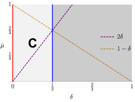
Figure 1: The region to the left of the vertical line at $\delta=\frac{1}{3}$ is where we assume small measurement degradation; in that region our extension of the KS theorem definitely demonstrates contextuality (C). In the region to the right, the degradation of the data is large and our extension of the KS theorem no longer refutes other explanations for the experimental data.

As is the case for conventional, infinitely-precise, quantum probability measures, the theorem is only applicable to dimensions $d\geq 3$. Indeed when the Hilbert space has dimension 2, it is straightforward to construct a 0-deterministic QIVPM as follows. Consider a non-contextual hidden variable model for $d=2$ (e.g., as proposed by Bell or Kochen-Specker Bell (1966); Kochen and Specker (1968)). Such a two-dimensional model assigns definite values to all observables at all times, and hence assigns a determinate probability (0 or 1) to each event. This probability measure directly induces a 0-deterministic QIVPM by changing 0 to F and 1 to T. It follows that every 0-deterministic QIVPM is $\delta$-deterministic.

IV.2 Experimental Data and $\delta$-determinism

Table 1: Possible probability measures on a Hilbert space of dimension $d=3$, where $\bar{\mu}_{2}^{\prime}$ and $\bar{\mu}_{3}$ are QIVPMs while $\bar{\mu}_{0}$, $\bar{\mu}_{1}$, and $\bar{\mu}_{2}$ are not. Events are listed in the column labeled by $P$.

$P$	$\bar{\mu}_{0}\left(P\right)$	$\bar{\mu}_{1}\left(P\right)$	$\bar{\mu}_{2}\left(P\right)$	$\bar{\mu}_{2}^{\prime}\left(P\right)$	$\bar{\mu}_{3}\left(P\right)$
$\mathbb{0}$	F	F	F	F	F
All one-dimensional projectors	$\left[0,0\right]$	$\left[0,\tfrac{1}{4}\right]$	$\left[0,\tfrac{1}{3}\right]$	$\left[\tfrac{1}{3},\tfrac{1}{3}\right]$	$\left[0,\tfrac{1}{2}\right]$
All two-dimensional projectors	$\left[1,1\right]$	$\left[\tfrac{3}{4},1\right]$	$\left[\tfrac{2}{3},1\right]$	$\left[\tfrac{2}{3},\tfrac{2}{3}\right]$	$\left[\tfrac{1}{2},1\right]$
$\mathbb{1}$	T	T	T	T	T

We have thus quantified one important aspect of uncertainty in quantum mechanics—the effect of the imprecise nature of devices—which is a novel addition to the theory of measurement. Indeed, as Heisenberg emphasized in his famous microscope example Heisenberg (1983), the conventional theory of measurement states that it is impossible to precisely measure any property of a system without disturbing it somewhat. Thus, there are fundamental limits to what one can measure and these limits have traditionally been attributed to complementarity. Our imprecision represents an additional source of indeterminacy beyond the inherent probabilistic nature of quantum mechanics.

In an experimental setup, $\delta$ is calculated as follows. To determine the probability of any event, we typically repeat an experiment $m$ times and count the number of times we witness the event. This assumes that for each run of the experiment we can determine, using our apparatus, whether the event occurred or not. Assume an event has an ideal mathematical probability of $0$, and we repeat the experiment $100$ times. In a perfect world we should be able to refute the event $100$ times and calculate that the probability is $0$. We might also observe the event $2$ times and refute it $98$ times and therefore calculate the probability to be $0.02$. Note that this situation assumes perfect measurement conditions and remains within the context of conventional (real-valued) probability theory. The question we focus on is what happens if we are only able to refute it $97$ times and are uncertain $3$ times? This is quite common in actual experiments. Mathematically we can model this idea by stating that the probability of the event is in the range $\left[0,0.03\right]$ which says that the probability of the event could be $0$, $0.01$, $0.02$, or $0.03$ as each the three uncertain records could either be evidence for the event or against it. We just cannot nail it down given the current experimental results and therefore represent the evidence as a ($\delta=$)$0.03$-deterministic probability measure. The interesting observation is that the axioms of probability theory (like additivity and convexity) impose enough constraints on the structure of interval-valued quantum probability measures to make them robust in the face of small non-vanishing $\delta$’s.

To see this idea in the context of a quantum experiment, consider a three-dimensional Hilbert space with one-dimensional projectors $P_{\rho}$, two-dimensional projectors $P_{\rho}+P_{\sigma}$, and an experiment that is repeated $12$ times. By the Kochen-Specker theorem, it is impossible to build a probability measure that maps every projection to either $0=\frac{0}{12}$ or $1=\frac{12}{12}$. That is, the assignment $\bar{\mu}_{0}$ defined in Table 1 is not a QIVPM.

Now consider what happens if $\frac{1}{4}$ of the data for every one-dimensional projector is uncertain. A potential account of this degradation is to assign to each event $P$ the entire range of possibilities $\bar{\mu}_{1}(P)$ as defined in Table 1. This measure is not a valid QIVPM because it does not satisfy the convexity condition: for any two orthogonal one-dimensional events $P_{0}$ and $P_{1}$, the convexity condition requires $\bar{\mu}_{1}\left(P_{0}+P_{1}\right)\subseteq\bar{\mu}_{1}\left(P_{0}\right)+\bar{\mu}_{1}\left(P_{1}\right)$, but $\bar{\mu}_{1}\left(P_{0}+P_{1}\right)=\left[\tfrac{3}{4},1\right]$ which is not a subset of $\left[0,\tfrac{1}{2}\right]=\bar{\mu}_{1}\left(P_{0}\right)+\bar{\mu}_{1}\left(P_{1}\right)$. Interestingly, it is impossible to find any probability measure that would be consistent with these observations, as the interval $\left[\tfrac{3}{4},1\right]$ is completely disjoint from the interval $\left[0,\tfrac{1}{2}\right]$ and no amount of shifting of assumptions regarding the precise outcome of the uncertain observations could change that disjointness. However, as shown next, a sharp transition occurs when $\delta=\tfrac{1}{3}$.

When the proportion of uncertain data reaches $\frac{1}{3}$, the probability measure that assigns to each event the entire range of possibilities is $\bar{\mu}_{2}$ defined in Table 1. This is also not a valid probability measure by the same argument as above. However, in this case $\bar{\mu}_{2}\left(P_{0}+P_{1}\right)=\left[\tfrac{2}{3},1\right]$ and $\left[0,\tfrac{2}{3}\right]=\bar{\mu}_{2}\left(P_{0}\right)+\bar{\mu}_{2}\left(P_{1}\right)$ have a common point. Hence, by assuming that the uncertain data for one-dimensional projectors always support the associated event, while those for two-dimensional projectors always refute the event, we can find the probability measure $\bar{\mu}_{2}^{\prime}$ that can verified to be a valid QIVPM and is consistent with the experimental data.

A similar situation happens when more than $\frac{1}{3}$ of data is uncertain. In particular, if half of the data is uncertain, the probability measure $\bar{\mu}_{3}$ that assigns to each event the entire range of possibilities is already a QIVPM.

V The Born Rule and Gleason’s Theorem

A conventional quantum probability measure can be easily constructed from a state $\rho$ according to the Born rule Born (1983); Mermin (2007); Jaeger (2007). According to Gleason’s theorem Gleason (1957); Redhead (1987); Peres (1995), this state $\rho$ is also the unique state consistent with any possible probability measure.

V.1 Finite-Precision Extension of Gleason’s Theorem

In order to re-examine these results in our framework, we first reformulate Gleason’s theorem in QIVPMs using infinitely precise uncountable intervals $\mathscr{I}_{\infty}=\left\{{\left[x,x\right]}\mathrel{}\middle|\mathrel{}{x\in\left[0,1\right]}\right\}$:

Theorem 4 ($\mathscr{I}_{\infty}$ Variant of the Gleason Theorem).

In a Hilbert space $\mathcal{H}$ of dimension $d\geq 3$, given a QIVPM $\bar{\mu}:\mathcal{E}\rightarrow\mathscr{I}_{\infty}$, the state $\rho$ consistent with $\bar{\mu}$ on every projector is unique, i.e., there exists a unique state $\rho$ such that $\overline{\mathcal{H}}\left(\bar{\mu},\mathcal{E}\right)=\{\rho\}$.

Now let us consider relaxing $\mathscr{I}$ to a countable set of finite-width intervals. As the intervals in the image of a QIVPM become less and less sharp, we expect more and more states to be consistent with it. In the limit of minimal sharpness, all states $\rho$ are consistent with the QIVPM

$$\bar{\mu}\left(P\right)=\begin{cases}{\textsf{{F}}}&\textrm{ if }P=\mathbb{0}\,;\\ {\textsf{{T}}}&\textrm{ if }P=\mathbb{1}\,;\\ {\textsf{{U}}}=\left[0,1\right]&\textrm{ otherwise}\end{cases}$$ (15)

mapping nearly all projections to the unknown interval U. There is however a subtlety: as shown in the theorem below, it is possible for an arbitrary assignment of intervals to projectors to be globally inconsistent.

Theorem 5 (Empty Cores Exist for General QIVPMs).

There exists a Hilbert space ${\cal H}$ and a QIVPM $\bar{\mu}:\mathcal{E}\rightarrow\mathscr{I}$ such that $\overline{\mathcal{H}}\left(\bar{\mu},\mathcal{E}\right)=\emptyset$.

To prove this theorem, we need to construct a QIVPM on some Hilbert space, and verify that there are no states that are consistent (see Defs. 2 and 3) with it on all possible events. Assume a Hilbert space of dimension $d=3$ with orthonormal basis $\left\{\ket{0},\ket{1},\ket{2}\right\}$, let $\ket{\texttt{+}}=\left(\ket{0}+\ket{1}\right)/\sqrt{2}$, $\ket{\texttt{+}^{\prime}}=\left(\ket{0}+\ket{2}\right)/\sqrt{2}$, and assign

$$\mathscr{I}_{0}=\left\{{\textsf{{T}}},{\textsf{{F}}},{\textsf{{U}}}\right\}\,.$$ (16)

The map $\bar{\mu}:\mathcal{E}\rightarrow\mathscr{I}_{0}$ defined in Table 2 can be verified to be a QIVPM Tai (forthcoming).

Table 2: QIVPM $\bar{\mu}:\mathcal{E}\rightarrow\mathscr{I}_{0}$ on a Hilbert space of dimension $d=3$. Events are listed in the column labeled by $P$.

$P$	$\bar{\mu}\left(P\right)$
$\mathbb{0}$, $\op{0}{0}$, $\op{\texttt{+}}{\texttt{+}}$, $\op{\texttt{+}^{\prime}}{\texttt{+}^{\prime}}$	F
$\mathbb{1}$, $\mathbb{1}-\op{0}{0}$, $\mathbb{1}-\op{\texttt{+}}{\texttt{+}}$, $\mathbb{1}-\op{\texttt{+}^{\prime}}{\texttt{+}^{\prime}}$	T
All other projectors	U

Next we will prove by contradiction that $\overline{\mathcal{H}}\left(\bar{\mu},\mathcal{E}\right)$ is the empty set. Suppose there is a state $\rho=\sum_{j=1}^{N}q_{j}\op{\phi_{j}}{\phi_{j}}\in\overline{\mathcal{H}}\left(\bar{\mu},\mathcal{E}\right)$, where $\sum_{j=1}^{N}q_{j}=1$ and $q_{j}>0$. Since we assumed the core $\overline{\mathcal{H}}\left(\bar{\mu},\mathcal{E}\right)$ is non-empty, so $\mu^{B}_{\rho}(P)\in\bar{\mu}(P)$, and Table 2 tells us that $\bar{\mu}(\op{0}{0})={\textsf{{F}}}=[0,0]$, we must conclude that $\mu^{B}_{\rho}(\op{0}{0})=0\in[0,0]$, and similarly for $\op{\texttt{+}}{\texttt{+}}$ and $\op{\texttt{+}^{\prime}}{\texttt{+}^{\prime}}$. If this is true, then $\ip{0}{\phi_{j}}=\ip{\texttt{+}}{\phi_{j}}=\ip{\texttt{+}^{\prime}}{\phi_{j}}=0$ for all $j$, and thus

$$\ip{1}{\phi_{j}}=\sqrt{2}\ip{\texttt{+}}{\phi_{j}}-\ip{0}{\phi_{j}}=0\,,$$ (17a)

$$\ip{2}{\phi_{j}}=\sqrt{2}\ip{\texttt{+}^{\prime}}{\phi_{j}}-\ip{0}{\phi_{j}}=0\,.$$ (17b)

The above equations imply $\ket{\phi_{j}}=\ket{0}\ip{0}{\phi_{j}}+\ket{1}\ip{1}{\phi_{j}}+\ket{2}\ip{2}{\phi_{j}}=0$, violating the assumption that $\ket{\phi_{j}}$ is a normalized state, and thus the theorem is proved.

The fact that a collection of poor measurements on a quantum system cannot reveal the underlying state is not surprising. Under certain conditions, we can however guarantee that the uncertainty in measurements is consistent with some non-empty collection of quantum states. Furthermore, we can relate the uncertainty in measurements to the volume of quantum states such that, in the limit of infinitely precise measurements, the volume of states collapses to a single state.

To that end, we introduce the concept of interval maps, which we can use to construct a consistent family of QIVPMs. An interval map $f:\left[0,1\right]\rightarrow\mathscr{I}$ maps every real-valued probability $x\in\left[0,1\right]$ to a set of intervals $f\left(x\right)=\left[\ell,r\right]$ containing $x$, where $\left[0,1\right]$ denotes the set of real-valued probabilities (this should not be confused with the interval-valued probability U). We also need a notion of norm to quantify the distance between (pure or mixed) states. The norm of a pure state $\rho=\op{\psi}{\psi}$ is defined as usual by $\left\|\psi\right\|=\sqrt{\ip{\psi}{\psi}}$. For any given Hermitian operator $A$, we choose the operator norm $\left\|A\right\|=\max_{\left\|\psi\right\|=1}\left\|A\ket{\psi}\right\|$, which is also known as the $2$-norm or the spectral norm Roberts and Varberg (1973); Peres (1995); Golub and Loan (1996); Foucart (2012). In fact, for any such matrix, including the density matrix $\rho$, this norm is the eigenvalue with maximum absolute value. Then, a finite-precision extension of Gleason’s theorem can be stated as follows:

Theorem 6 (Finite-Precision Extension of the Gleason Theorem).

Let $f:\left[0,1\right]\rightarrow\mathscr{I}$ be an interval map and let the composition $f\circ\mu^{B}_{\rho}$ be a QIVPM, where $\mu^{B}_{\rho}$ is the probability measure induced by the Born rule for a given state $\rho$. Let $\alpha$ be the maximum length of intervals in $\mathscr{I}$. If a state $\rho^{\prime}$ is consistent with $f\circ\mu^{B}_{\rho}$ on all events, i.e., $\rho^{\prime}\in\overline{\mathcal{H}}\left(f\circ\mu^{B}_{\rho},\mathcal{E}\right)$, then the norm of their difference is bounded by $\alpha$, i.e., $\left\|\rho-\rho^{\prime}\right\|\leq\alpha$.

The proof proceeds as follows. Given a state $\rho^{\prime}$ consistent with $f\circ\mu^{B}_{\rho}$, we have $\mu^{B}_{\rho^{\prime}}\left(\op{\psi}{\psi}\right)\in f\left(\mu^{B}_{\rho}\left(\op{\psi}{\psi}\right)\right)$ for any one-dimensional projector $P=\op{\psi}{\psi}$. Since the maximum length of the intervals in $\mathscr{I}$ is $\alpha$, it is also the upper bound of the difference:

$$\left|\mu^{B}_{\rho^{\prime}}\left(\op{\psi}{\psi}\right)-\mu^{B}_{\rho}\left(\op{\psi}{\psi}\right)\right|=\left|\melem{\psi}{\rho-\rho^{\prime}}{\psi}\right|\leq\alpha\,.$$

Since $\rho-\rho^{\prime}$ is Hermitian, $\max_{\left\|\psi\right\|=1}\left|\melem{\psi}{\rho-\rho^{\prime}}{\psi}\right|$ is the maximum absolute value of the eigenvalues of $\rho-\rho^{\prime}$ Nielsen and Chuang (2000), and equal to $\left\|\rho-\rho^{\prime}\right\|$ Golub and Loan (1996); Foucart (2012). Hence, $\left\|\rho-\rho^{\prime}\right\|\leq\alpha$.

V.2 Ultramodular Functions

Theorem 6 generalizes Gleason’s theorem in the sense that it accounts for a larger class of probability measures that includes the conventional one as a limit. The theorem is however “special” in the sense that it only applies to the particular class of QIVPMs constructed by composing an interval map with a conventional quantum probability measure. QIVPMs constructed in this manner have some peculiar properties that we examine next.

An interval map is called ultramodular if it satisfies the following properties:

Definition 6 (Ultramodular Functions).

Given a collection of intervals $\mathscr{I}$ including F and T, an interval map $\mathcal{M}:\left[0,1\right]\rightarrow\mathscr{I}$ is called ultramodular if:

$$\mathcal{M}(0)={\textsf{{F}}}\,,$$ (18a)

$$\mathcal{M}(1)={\textsf{{T}}}\,,$$ (18b)

$$\mathcal{M}\left(1-x\right)={\textsf{{T}}}-\mathcal{M}\left(x\right)\,,$$ (18c)

and for any three numbers $x_{0}$, $x_{1}$, and $x_{2}\in\left[0,1\right]$ such that $y=x_{0}+x_{1}+x_{2}\in\left[0,1\right]$, we have:

$$\mathcal{M}\left(y\right)+\mathcal{M}\left(x_{2}\right)\subseteq\mathcal{M}\left(x_{0}+x_{2}\right)+\mathcal{M}\left(x_{1}+x_{2}\right)\,.$$ (19)

The first three constraints, Eqs. (18), are the direct counterpart of the corresponding QIVPM constraints, Eqs. (6); the last condition, Eq. (19), is the direct counterpart of the convexity conditions, Eqs. (4) and (7) Choquet (1954); Shapley (1971); Ng et al. (1997); Marinacci and Montrucchio (2005). Therefore, these conditions guarantee that, for any conventional quantum probability measure $\mu$, the composition $\mathcal{M}\circ\mu$ defines a valid QIVPM. Conversely, if for every quantum probability measure $\mu$, it is the case that $f\circ\mu$ is a QIVPM, then the interval map $f$ is an ultramodular function. Formally, we have the following result:

Theorem 7 (Equivalence of Ultramodular Functions and IVPMs).

The following three statements are equivalent:

1. A function $\mathcal{M}:\left[0,1\right]\rightarrow\mathscr{I}$ is ultramodular.

2. The composite function $\mathcal{M}\circ\mu:\mathcal{E}_{C}\rightarrow\mathscr{I}$ is a classical IVPM for all classical probability measures $\mu:\mathcal{E}_{C}\rightarrow\left[0,1\right]$.

3. The composite function $\mathcal{M}\circ\mu:\mathcal{E}\rightarrow\mathscr{I}$ is a QIVPM for all quantum probability measures $\mu:\mathcal{E}\rightarrow\left[0,1\right]$.

Statement 1 implies 2 and 3 as we have outlined above. Conversely, for the quantum case, we want to show that if $\mathcal{M}$ is not ultramodular, then for some quantum probability measure $\mu$, the composite $\mathcal{M}\circ\mu$ might not be a QIVPM. Suppose there are three particular numbers $x_{0}$, $x_{1}$, and $x_{2}\in\left[0,1\right]$ such that $y=x_{0}+x_{1}+x_{2}\in\left[0,1\right]$, but they don’t satisfy Eq. (19). Consider the state:

$$\rho=x_{0}\op{0}{0}+x_{1}\op{1}{1}+x_{2}\op{2}{2}+\left(1-y\right)\op{3}{3}\,.$$

The induced map $\mathcal{M}\circ\mu^{B}_{\rho}$ constructed using the Born rule and blurred by $\mathcal{M}$ fails to satisfy Eq. (7) when $P_{0}=\op{0}{0}+\op{2}{2}$ and $P_{1}=\op{1}{1}+\op{2}{2}$. In other words, this induced map fails to be a QIVPM. For the classical case, if $\mathcal{M}$ is not ultramodular, we also want to find a classical probability measure $\mu:\mathcal{E}_{C}\rightarrow\left[0,1\right]$ such that $\mathcal{M}\circ\mu$ is not a classical IVPM. This can be done by restricting our previous quantum probability measure $\mu^{B}_{\rho}$ to the space of events $\mathcal{E}_{C}$ generated by the mutually commuting projectors $\op{0}{0}$, $\op{1}{1}$, $\op{2}{2}$, and $\op{3}{3}$. The restricted function $\mu=\mu^{B}_{\rho}|_{\mathcal{E}_{C}}$ is then a classical probability measure, and the induced map $\mathcal{M}\circ\mu$ fails to be a classical IVPM for the same reason as in the quantum case.

In other words, essential properties of QIVPMs constructed using interval maps can be gleaned from the properties of ultramodular functions. The following is a most interesting property in our setting:

Theorem 8 (Range of Ultramodular Functions).

For any ultramodular function $\mathcal{M}:\left[0,1\right]\rightarrow\mathscr{I}$, either $\mathscr{I}=\mathscr{I}_{0}$ as defined in Eq. (16) or $\mathscr{I}$ contains uncountably many intervals.

Since $\mathcal{M}$ maps to intervals, we can decompose it into two functions: its left-end and right-end, where $\left[\mathcal{M}^{L{}}\left(x\right),\mathcal{M}^{R{}}\left(x\right)\right]=\mathcal{M}\left(x\right)$. By Eq. (19), the left-end function $\mathcal{M}^{L{}}:\left[0,1\right]\rightarrow\left[0,1\right]$ is Wright-convex Wright (1954); Roberts and Varberg (1973); Pečarić et al. (1992), i.e.,

$$\mathcal{M}^{L{}}\left(y\right)+\mathcal{M}^{L{}}\left(x_{2}\right)\geq\mathcal{M}^{L{}}\left(x_{0}+x_{2}\right)+\mathcal{M}^{L{}}\left(x_{1}+x_{2}\right)$$

for three numbers $x_{0}$, $x_{1}$, and $x_{2}\in\left[0,1\right]$ with $y=x_{0}+x_{1}+x_{2}\in\left[0,1\right]$. Together with the fact that $\mathcal{M}^{L{}}$ maps to a bounded interval $\left[0,1\right]$, the left-end function $\mathcal{M}^{L{}}$ must be continuous on the unit open interval $\left(0,1\right)$ Marinacci and Montrucchio (2005). Therefore, either $\mathcal{M}$ maps every number in $\left(0,1\right)$ to the same interval, or the number of intervals to which $\mathcal{M}$ maps must be uncountable.

To summarize, a conventional quantum probability measure has an uncountable range $[0,1]$. A QIVPM constructed by blurring such a conventional quantum probability measure must also have an uncountable range of intervals. Of course, any particular QIVPM, or any particular experiment, will use a fixed collection of intervals appropriate for the resources and precision of the particular experiment.

VI Conclusion

Foundational concepts in quantum mechanics, such as the Kochen-Specker and Gleason theorems, rely in subtle ways on the use of unbounded resources. By assuming infinitely precise measurements, these two insightful theorems form the foundations of two fundamental aspects of quantum mechanics. On the one hand, the Kochen-Specker result reveals a distinctive aspect of physical reality, the fact that it is contextual, and, on the other hand, Gleason’s theorem establishes a relationship between quantum states and probabilities uniquely defined by Born’s rule. Our goal in this paper has been to analyze the physical consequences of a mathematical framework that allows for finite precision measurements by introducing the concept of quantum interval-valued probability. This framework incorporates uncertainty in the measurement results by defining fuzzy probability measures, and includes standard quantum measurement as the particular instance of sharp, infinitely precise, intervals.

In addition, we showed how these two theorems emerge as limiting cases of this same framework, thus connecting two seemingly unrelated aspects of quantum physics. We noted that arbitrary finite precision measurement conditions can nullify the main tenets of both theorems. However, by carefully specifying experimental uncertainties, we were able to establish rigorous bounds on the validity of these two theorems. Therefore, we have established a context in which infinite precision quantum mechanical theories can be reconciled with finite precision quantum mechanical measurements, and have provided a possible resolution of the Meyer-Mermin debate on the impact of finite precision on the Kochen-Specker theorem Meyer (1999); Mermin (1999).