Efficient Algorithms for t-distributed Stochastic Neighborhood Embedding

Abstract.

t-distributed Stochastic Neighborhood Embedding (t-SNE) is a method for dimensionality reduction and visualization that has become widely popular in recent years. Efficient implementations of t-SNE are available, but they scale poorly to datasets with hundreds of thousands to millions of high dimensional data-points. We present Fast Fourier Transform-accelerated Interpolation-based t-SNE (FIt-SNE), which dramatically accelerates the computation of t-SNE. The most time-consuming step of t-SNE is a convolution that we accelerate by interpolating onto an equispaced grid and subsequently using the fast Fourier transform to perform the convolution. We also optimize the computation of input similarities in high dimensions using multi-threaded approximate nearest neighbors. We further present a modification to t-SNE called “late exaggeration,” which allows for easier identification of clusters in t-SNE embeddings. Finally, for datasets that cannot be loaded into the memory, we present out-of-core randomized principal component analysis (oocPCA), so that the top principal components of a dataset can be computed without ever fully loading the matrix, hence allowing for t-SNE of large datasets to be computed on resource-limited machines.

1. Introduction

In many fields, the visualization of large, high-dimensional datasets is essential. t-distributed Stochastic Neighborhood Embedding (t-SNE), introduced by van der Maaten and Hinton (2008), has become enormously popular in many fields, such as in the analysis of single-cell RNA-sequencing (scRNA-seq) data, where it is used to discover the subpopulations among large numbers of cells in an unsupervised fashion. Unfortunately, even efficient methods for approximate t-SNE require many hours to embed datasets on the order of hundreds of thousands to millions of points, as often encountered in scRNA-seq and elsewhere. In this paper, we present Fast Fourier Transform-accelerated Interpolation-based t-SNE (FIt-SNE) for fast and accurate computation of t-SNE, essentially making it feasible to use t-SNE on datasets of this scale. Furthermore, we build on recent theoretical advances to more clearly separate clusters in t-SNE embeddings. Finally, we present an out-of-core implementation of randomized principal component analysis (oocPCA) so that users can embed datasets that are too large to load in the memory.

1.1. t-distributed Stochastic Neighborhood Embedding

Given a $d$-dimensional dataset $X=\{x_{1},x_{2},...,x_{N}\}\subset\mathbb{R}^{d}$, t-SNE aims to compute the low dimensional embedding $Y=\{y_{1},y_{2},...,y_{N}\}\subset\mathbb{R}^{s}$ where $s\ll d$, such that if two points $x_{i}$ and $x_{j}$ are close in the input space, then their corresponding points $y_{i}$ and $y_{j}$ are also close. Affinities between points $x_{i}$ and $x_{j}$ in the input space, $p_{ij}$, are defined as

$$p_{i|j}=\frac{\exp{(-\|x_{i}-x_{j}\|^{2}/2\sigma_{i}^{2})}}{\sum_{k\neq i}\exp{(-\|x_{i}-x_{k}\|^{2}/2\sigma_{i}^{2}})}\qquad\mbox{and}\qquad p_{ij}=\frac{p_{i|j}+p_{j|i}}{2N}.$$

$\sigma_{i}$ is the bandwidth of the Gaussian distribution, and it is chosen using such that the perplexity of $P_{i}$ matches a given value, where $P_{i}$ is the conditional distribution of all the other points given $x_{i}$. Similarly, the affinity between points $y_{i}$ and $y_{j}$ in the embedding space is defined using the Cauchy kernel

$$q_{ij}=\frac{(1+\|y_{i}-y_{j}\|^{2})^{-1}}{\sum_{k\neq l}(1+\|y_{k}-y_{l}\|^{2})^{-1}}.$$

t-SNE finds the points $\{y_{1},...,y_{n}\}$ that minimize the Kullback-Leibler divergence between the joint distribution of points in the input space $P$ and the joint distribution of the points in the embedding space $Q$,

$$C(\mathcal{Y})=KL(P||Q)=\sum_{i\neq j}p_{ij}\log\frac{p_{ij}}{q_{ij}}.$$

Starting with a random initialization, the cost function $C(\mathcal{Y})$ is minimized by gradient descent, with the gradient (as derived by van der Maaten and Hinton (2008))

$$\frac{\partial C}{\partial y_{i}}=4\sum\limits_{j\neq i}(p_{ij}-q_{ij})q_{ij}Z(y_{i}-y_{j}),$$

where $Z$ is a global normalization constant

$$Z=\sum_{k\neq l}{\left(1+\|y_{k}-y_{l}\|^{2}\right)^{-1}}.$$

We split the gradient into two parts

$$\frac{1}{4}\frac{\partial C}{\partial y_{i}}=\sum_{j\neq i}{p_{ij}q_{ij}Z(y_{i}-y_{j})}-\sum_{j\neq i}{q_{ij}^{2}Z(y_{i}-y_{j})}$$

where the first sum $F_{\text{attr},i}$ corresponds to an attractive force between points and the second sum $F_{\text{rep},i}$ corresponds to a repulsive force

$$\frac{1}{4}\frac{\partial C}{\partial y_{i}}=F_{\text{attr},i}-F_{\text{rep},i}.$$

The computation of the gradient at each step is an $n$-body simulation, where the position of each point is determined by the forces exerted on it by all other points. Exact computation of $n$-body simulations scales as $O(n^{2})$, making exact t-SNE computationally prohibitive for datasets with tens of thousands of points. Accordingly, van der Maaten (2014)’s popular implementation of t-SNE produces an approximate solution, and can be used on larger datasets. In that implementation, they approximate $F_{\text{attr},i}$ by nearest neighbors as computed using vantage-point trees (Yianilos (1993)). Since the input similarities do not change, they can be precomputed, and hence do not dominate the computational time. On the other hand, the repulsive forces $F_{\text{rep},i}$ are approximated at each iteration using the Barnes-Hut Algorithm (Barnes and Hut (1986)), a tree-based algorithm which scales as $O(n\log n)$. Despite these accelerations, it can still take many hours to run t-SNE on large scRNA-seq datasets. Furthermore, given that t-SNE is often run many times with different initializations to find the best embedding, faster algorithms are needed. In this work, we present an approximate nearest neighbor based implementation for computing $F_{\text{attr},i}$ and an interpolation-based fast Fourier transform accelerated algorithm for computing $F_{\text{repul},i}$, both of which are significantly faster than current methods.

1.2. Early exaggeration

van der Maaten (2014) and van der Maaten and Hinton (2008) note that as the number of points $n$ increases, the convergence rate slows down. To circumvent this problem, implementations of t-SNE multiply the $F_{\text{attr},i}$ term by a constant $\alpha>1$ during the first $250$ iterations of gradient descent:

$$\frac{1}{4}\frac{\partial C}{\partial y_{i}}=\alpha F_{\text{attr},i}-F_{\text{rep},i}$$

This “early exaggeration” forces the points into tight clusters which can move more easily, and are hence less likely to get trapped in local minima. Linderman and Steinerberger (2017) showed that this early exaggeration phase is essential for convergence of the algorithm and that when the exaggeration coefficient $\alpha$ is set optimally, t-SNE is guaranteed to recover well-separated clusters. In Section §4 we show that late exaggeration (i.e. setting $\alpha>1$ during the last several hundred iterations) is also useful, and can result in improved separation of clusters.

1.3. Organization

The organization of this paper is as follows: we first present and benchmark a fast Fourier transform accelerated interpolation-based method for optimizing the computation of $F_{\text{rep},i}$ in Section §2. Section §3 describes methods for accelerating the computation of input similarities $p_{ij}$ required for $F_{\text{attr},i}$. Section §4 describes “late exaggeration” for improving separation of clusters in t-SNE embeddings. Section §5 describes t-SNE heatmaps, an application of 1-dimensional t-SNE to the visualization of single-cell RNA-sequencing data. Finally, Section §6 presents an implementation of out-of-core PCA for the analysis of datasets too large to fit in the memory.

2. The repulsive forces $F_{\text{rep},i}$

Suppose $\{y_{1},y_{2},\dots,y_{N}\}$ is an $s$-dimensional embedding of a collection of $d$-dimensional vectors $\{x_{1},\dots,x_{N}\}.$ At each step of gradient descent, the repulsive forces are given by

(1) $$F_{\text{rep},k}(m)=\left(\sum_{\begin{subarray}{c}\ell=1\\ \ell\neq k\end{subarray}}^{N}\frac{y_{\ell}(m)-y_{k}(m)}{\left(1+\|y_{\ell}-y_{k}\|^{2}\right)^{2}}\right)\Bigg{/}\left(\mathop{\sum_{\begin{subarray}{c}j=1\end{subarray}}^{N}\sum_{\begin{subarray}{c}\ell=1\end{subarray}}^{N}}_{\ell\neq j}\frac{1}{(1+\|y_{\ell}-y_{j}\|^{2})}\right)\,,$$

where $k=1,2,\ldots N$, $m=1,2\ldots s,$ and $y_{i}(j)$ denotes the $j^{\rm th}$ component of $y_{i}.$ Evidently, the repulsive force between the vectors $\{y_{1},\dots,y_{N}\}$ consists of $N^{2}$ pairwise interactions, and were it computed directly, would require CPU-time scaling as $O(N^{2}).$ Even for datasets consisting of a few thousand points, this cost becomes prohibitively expensive. Our approach enables the accurate computation of these pairwise interactions in $O(N)$ time. Since the majority of applications of t-SNE are for two-dimensional embeddings (and in §5 we present an application of one-dimensional embeddings), in the following we focus our attention on the cases where $s=1$ or $2.$ However, we note that our algorithm extends naturally to arbitrary dimensions. In such cases, though the constants in the computational cost will vary, our approach will still yield an algorithm with a CPU-time which scales as $O(N).$

We begin by observing that the repulsive forces $F_{\text{rep},k}$ defined in eq. 1 can be expressed as $s+2$ sums of the form

(2) $$\phi(y_{i})=\sum_{j=1}^{N}K(y_{i},y_{j})q_{j}$$

where the kernel $K(y,z)$ is either

(3) $$K_{1}(y,z)=\frac{1}{(1+\|y-z\|^{2})}\,,\quad\text{or}\quad K_{2}(y,z)=\frac{1}{(1+\|y-z\|^{2})^{2}}\,,$$

for $y,z\in\mathbb{R}^{s}$ (see Appendix). Note that both of the kernels $K_{1}$ and $K_{2}$ are smooth functions of $y,z$ for all $y,z\in\mathbb{R}^{s}$. The key idea of our approach is to use polynomial interpolants of the kernel $K$ in order to accelerate the evaluation of the $N-$body interactions defined in eq. 2.

2.1. Mathematical Preliminaries

First, we demonstrate with a simple example how polynomial interpolation can be used to accelerate the computation of the $N-$body interactions with a smooth kernel. Suppose that $y_{1},\dots,y_{M}\in(y_{0},y_{0}+R)$ and $z_{1},\dots,z_{N}\in(z_{0},z_{0}+R)$. Let $I_{y_{0}}$ and $I_{z_{0}}$ denote the intervals $(y_{0},y_{0}+R)$ and $(z_{0},z_{0}+R)$, respectively. Note that no assumptions are made regarding the relative locations of $y_{0}$ and $z_{0};$ in particular, the case $y_{0}=z_{0}$ is also permitted.

Now consider the sums

(4) $$\phi(y_{i})=\sum_{j=1}^{N}K(y_{i},z_{j})q_{j}\,,\quad i=1,2,\ldots M\,.$$

Let $p$ be a positive integer. Suppose that $\tilde{z}_{1},\dots,\tilde{z}_{p},$ are a collection of $p$ points on the interval $I_{z_{0}}$ and that $\tilde{y}_{1},\dots,\tilde{y}_{p}$, are a collection of $p$ points on the interval $I_{y_{0}}$. Let $K_{p}(y,z)$ denote a bivariate polynomial interpolant of the kernel $K(y,z)$ satisfying

$$K_{p}(\tilde{y}_{j},\tilde{z}_{\ell})=K(\tilde{y}_{j},\tilde{z}_{\ell})\,,\quad j,\ell=1,2,\ldots p.$$

A simple calculation shows that $K_{p}(y,z)$ is given by

(5) $$K_{p}(y,z)=\sum_{\ell=1}^{p}\sum_{j=1}^{p}K(\tilde{y}_{j},\tilde{z}_{\ell})L_{j,\tilde{y}}(y)L_{\ell,\tilde{z}}(z)\,,$$

where $L_{j,\tilde{y}}(y)$ and $L_{\ell,\tilde{z}}(z)$ are the Lagrange polynomials

$$L_{\ell,\tilde{y}}(y)=\prod_{\begin{subarray}{c}j=1\\ j\neq\ell\end{subarray}}^{p}(y-\tilde{y}_{j})\Big{/}\prod_{\begin{subarray}{c}j=1\\ j\neq\ell\end{subarray}}^{p}(\tilde{y}_{\ell}-\tilde{y}_{j})\,,\quad\text{and}\quad L_{\ell,\tilde{z}}(z)=\prod_{\begin{subarray}{c}j=1\\ j\neq\ell\end{subarray}}^{p}(z-\tilde{z}_{j})\Big{/}\prod_{\begin{subarray}{c}j=1\\ j\neq\ell\end{subarray}}^{p}(\tilde{z}_{\ell}-\tilde{z}_{j})\,,$$

$\ell=1,2\ldots p$. In the following we will refer to the points $\tilde{y}_{1},\dots,\tilde{y}_{p}$, and $\tilde{z}_{1},\dots,\tilde{z}_{p}$ as interpolation points.

Let $\tilde{\phi}(y_{i})$ denote the approximation to $\phi(y_{i})$ obtained by replacing the kernel $K$ in  eq. 4 by its polynomial interpolant $K_{p}$, i.e.

$$\tilde{\phi}(y_{i})=\sum_{j=1}^{N}K_{p}(y_{i},z_{j})q_{j}\,,$$

for $i=1,2\ldots M$. Clearly the error in approximating $\phi(y_{i})$ via $\tilde{\phi}(y_{i})$ is bounded (up to a constant) by the error in approximating $K(y,z)$ via $K_{p}(y,z)$. In particular, if the polynomial interpolant satisfies the inequality

$$\sup_{\begin{subarray}{c}y\in(y_{0},y_{0}+R)\\ z\in(z_{0},z_{0}+R)\end{subarray}}|K_{p}(y,z)-K(y,z)|\leq\varepsilon\,,$$

then the error $|\tilde{\phi}(y_{i})-\phi(y_{i})|$ is given by

$$|\tilde{\phi}(y_{i})-\phi(y_{i})| =\left|\sum_{j=1}^{N}\left(K_{p}(y_{i},z_{j})-K(y_{i},z_{j})\right)q_{j}\right|$$

$$\leq\sum_{j=1}^{N}\left|K_{p}(y_{i},z_{j})-K(y_{i},z_{j})\right||q_{j}|$$

$$\leq\varepsilon\sum_{j=1}^{N}|q_{j}|\,.$$

A direct computation of $\phi(y_{1}),\dots,\phi(y_{M})$ requires $O(M\cdot N)$ operations. On the other hand, the values $\tilde{\phi}(y_{i})$, $i=1,2,\ldots M$, can be computed in $O((M+N)\cdot p+p^{2})$ operations as follows. Using eq. 5, $\tilde{\phi}(y_{i})$ can be rewritten as

$$\tilde{\phi}(y_{i}) =\sum_{j=1}^{N}\sum_{\ell=1}^{p}\sum_{m=1}^{p}K(\tilde{y}_{\ell},\tilde{z}_{m})L_{\ell,\tilde{y}}(y_{i})L_{m,\tilde{z}}(z_{j})q_{j}\,,$$

$$=\sum_{\ell=1}^{p}L_{\ell,\tilde{y}}(y_{i})\left(\sum_{m=1}^{p}K(\tilde{y}_{\ell},\tilde{z}_{m})\left(\sum_{j=1}^{N}L_{m,\tilde{z}}(z_{j})q_{j}\right)\right)\,,$$

for $i=1,2,\ldots M$. The values $\tilde{\phi}(y_{1}),\dots,\tilde{\phi}(y_{M})$, are computed in three steps.

• Step 1: Compute the coefficients $w_{m}$ defined by the formula

  $$w_{m}=\sum_{j=1}^{N}L_{m,\tilde{z}}(z_{j})q_{j}\,,$$

  for each $m=1,2,\ldots p$. This step requires $O(N\cdot p)$ operations.

• Step 2: Compute the values $v_{\ell}$ at the interpolation nodes $\tilde{y}_{\ell}$ defined by the formula

  $$v_{\ell}=\sum_{m=1}^{p}K(\tilde{y}_{\ell},\tilde{z}_{m})w_{m}$$

  for all $\ell=1,2,\ldots p$. This step requires $O(p^{2})$ operations.

• Step 3: Evaluate the potential $\tilde{\phi}(y_{i})$ using the formula

  $$\tilde{\phi}(y_{i})=\sum_{\ell=1}^{p}L_{\ell,\tilde{y}}(y_{i})v_{\ell}\,,$$

  for all $i=1,2\ldots M$. This step requires $O(M\cdot p)$ operations.

See fig. 1 for an illustrative figure of the above procedure.

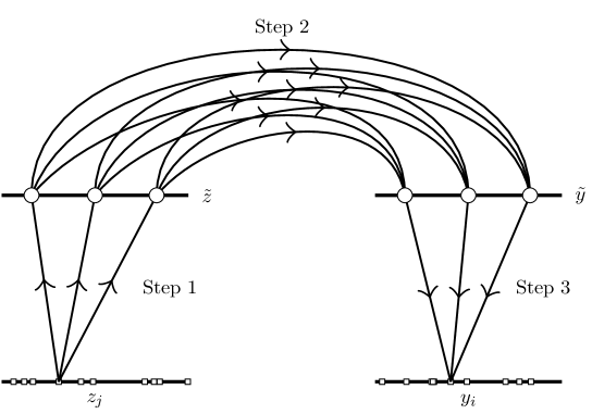
Figure 1. An illustration of the algorithm. Both the intervals on the left are $(z_{0},z_{0}+R)$, and both the intervals on the right are $(y_{0},y_{0}+R)$. In the lower intervals, the white squares denote the locations $z_{j}$ and $y_{i}$, and in the upper intervals the white circles indicate the locations of the equispaced nodes $\tilde{z}_{i}$, and $\tilde{z}_{j}$. The arrow illustrate how a point $z_{j}$ communicates with a point $y_{i}$.

2.2. Algorithm

In this section, we present the main algorithm for the rapid evaluation of the repulsion forces eq. 2. The central strategy is to use piecewise polynomial interpolants of the kernel with equispaced points, and use the procedure described in Section §2.1.

Specifically, suppose that the points $y_{i}$, $i=1,2,\ldots N$ are all contained in the interval $[y_{\mathrm{min}},y_{\mathrm{max}}]$. We subdivide the interval $[y_{\mathrm{min}},y_{\mathrm{max}}]=\bigcup_{i=1}^{N_{\text{int}}}I_{j}$, into $N_{\text{int}}$ intervals of equal length. Let $\tilde{y}_{j,\ell}$ denote $p$ equispaced nodes on the interval $I_{\ell}$ given by

(6) $$\tilde{y}_{j,\ell}=h/2+((j-1)+(\ell-1)\cdot p)\cdot h\,,$$

where $h=1/(N_{\text{int}}\cdot p)$, $j=1,2\ldots p$, and $\ell=1,2\ldots N_{\text{int}}$.

Remark 1.

The nodes $\tilde{y}_{j,\ell}$, $j=1,2\ldots p$, and $\ell=1,2,\ldots N_{\text{int}}$, defined in eq. 6, are also equispaced on the whole interval $[y_{\mathrm{min}},y_{\mathrm{max}}]$.

The interaction between any two intervals $I$, $J$, i.e.

$$\sum_{y_{j}\in J}K(y_{i},y_{j})q_{j}\,,\quad y_{i}\in I$$

can be accelerated via the algorithm discussed in section 2.1. This procedure amounts to using a piecewise polynomial interpolant of the kernel $K(y,z)$ on the domain $y,z\in[y_{\mathrm{min}},y_{\mathrm{max}}]$ as opposed to using an interpolant on the whole interval. We summarize the procedure below.

• Step 1: For each interval $I_{\ell}$, $\ell=1,2,\ldots N_{\text{int}}$, compute the coefficients $w_{m,\ell}$ defined by the formula

  $$w_{m,\ell}=\sum_{y_{j}\in I_{\ell}}L_{m,\tilde{y}^{\ell}}(y_{j})q_{j}\,,$$

  for each $m=1,2,\ldots p$. This step requires $O(N\cdot p)$ operations.

• Step 2: Compute the values $v_{m,n}$ at the equispaced nodes $\tilde{y}_{m,n}$ defined by the formula

  (7) $$v_{m,n}=\sum_{j=1}^{N_{\text{int}}}\sum_{\ell=1}^{p}K(\tilde{y}_{m,n},\tilde{y}_{\ell,j})w_{\ell,j}$$

  for all $m=1,2,\ldots p$, $n=1,2\ldots N_{\text{int}}$. This step requires $O((N_{\text{int}}\cdot p)^{2})$ operations.

• Step 3: For each interval $I_{\ell}$, $\ell=1,2,\ldots N_{\text{int}}$, compute the potential $\phi(y_{i})$ via the formula

  $$\phi(y_{i})=\sum_{j=1}^{p}L_{j,\tilde{y}^{\ell}}(y_{i})v_{j,\ell}\,,$$

  for all points $y_{i}\in I_{\ell}$. This step requires $O(N\cdot p)$ operations.

In this procedure, the functions $L_{j,\tilde{y}^{\ell}}$, $j=1,2,\ldots p$, are the Lagrange polynomials corresponding to the equispaced interpolation nodes on interval $I_{\ell}$.

In Step 2 of the above procedure, we are evaluating $N-$body interactions on equispaced grid points. For notational convenience, we rewrite the sum eq. 7

(8) $$v_{i}=\sum_{j=1}^{N_{\text{int}}\cdot p}K(\tilde{y}_{i},\tilde{y}_{j})w_{j}\,,$$

$i=1,2,\ldots N_{\text{int}}\cdot p$. The kernels of interest ($K_{1}$ and $K_{2}$ defined in eq. 3) are translationally-invariant, i.e., the kernels satisfy $K(y,z)=K(y+\delta,z+\delta)$ for any $\delta$. The combination of using equispaced points, along with the translational-invariance of the kernel, implies that the matrix associated with the evaluation of the sums eq. 8 is Toeplitz. This computation can thus be accelerated via the fast-Fourier transform (FFT), which reduces the computational complexity of evaluating the sums eq. 8 from $O((N_{\text{int}}\cdot p)^{2})$ operations to $O(N_{\text{int}}\cdot p\log{(N_{\text{int}}\cdot p)})$.

Algorithm 1 describes the fast algorithm for evaluating the repulsive forces eq. 2 in one dimension (s=1) which has computational complexity $O(N\cdot p+(N_{\text{int}}\cdot p)\log{(N_{\text{int}}\cdot p)})$ .

Input: Collection of points $\{y_{i}\}_{i=1}^{N}$, source strengths $\{q_{i}\}_{i=1}^{N}$, number of intervals $N_{\text{int}}$, number of interpolation points per interval $p$

1

Output: $\phi(y_{i})=\sum_{j=1}^{N}K(y_{i},y_{j})q_{j}$ for $i=1,2\ldots N$

2

3For each interval $I_{\ell}$, form the equispaced nodes $\tilde{y}_{j,\ell}$, $j=1,2,\ldots p$ given by eq. 6

4for $I\leftarrow 1$ to $N_{\text{int}}$ do

5      Compute the coefficients $w_{m,\ell}$ given by

$$w_{m,\ell}=\sum_{y_{i}\in I_{\ell}}L_{m,\tilde{y}^{\ell}}(y_{i})q_{i}\,,$$

$m=1,2,\ldots p$.

6 end for

7

8Use the fast-Fourier transform to compute the values of $v_{m,n}$ given by

(9) $$\begin{bmatrix}v_{1,1}\\ v_{2,1}\\ \vdots\\ v_{p-1,N_{\text{int}}}\\ v_{p,N_{\text{int}}}\end{bmatrix}=\tilde{K}\cdot\begin{bmatrix}w_{1,1}\\ w_{2,1}\\ \vdots\\ w_{p-1,N_{\text{int}}}\\ w_{p,N_{\text{int}}}\end{bmatrix}\,,$$

where $\tilde{K}$ is the Toeplitz matrix given by

(10) $$\tilde{K}_{i,j}=K(\tilde{y}_{i},\tilde{y}_{j})\,,$$

$i,j=1,2,\ldots N_{\text{int}}\cdot p$.

9for $I\leftarrow 1$ to $N_{\text{int}}$ do

10       Compute $\phi(y_{i})$ at all points $y_{i}\in I_{\ell}$ via

$$\phi(y_{i})=\sum_{j=1}^{p}L_{j,\tilde{y}^{\ell}}(y_{i})v_{j,\ell}$$

11 end for

Algorithm 1 FFT-accelerated Interpolation-based t-SNE (FIt-SNE)

2.3. Optimal choice of $p$ and $N_{\text{int}}$

Recall that the computational complexity of Algorithm 1 is $O(N\cdot p+N_{\text{int}}\cdot p\log{(N_{\text{int}}\cdot p)})$. We remark that the choice of the parameters $N_{\text{int}}$ and $p$ depends solely on the specified tolerance $\varepsilon$ and is independent of the number of points $N$. Generally, increasing $p$ will reduce the number of intervals $N_{\text{int}}$ required to obtain the same accuracy in the computation. However, we observe that the reduction in $N_{\text{int}}$ for an increased $p$ is not advantageous from a computational perspective—since, as the number of points $N$ increases, the computational cost is independent of $N_{\text{int}}$ and is only a function of $p$. Moreover, for the t-SNE kernels $K_{1}$ and $K_{2}$ defined in eq. 3, it turns out that for a fixed accuracy the product $N_{\text{int}}\cdot p$ remains nearly constant for $p\geq 3$. Thus, it is optimal to use $p=3$ for all t-SNE calculations. In a more general environment, when higher accuracy is required and for other translationally invariant kernels $K$, the choice of the number of nodes per interval $p$ and the total number of intervals $N_{\text{int}}$ can be optimized based on the accuracy of computation required.

Remark 2.

Special care must be taken when increasing $p$ in order to achieve higher accuracy due to the Runge phenomenon associated with equispaced nodes. In fact, the kernels that arise in t-SNE are archetypical examples of this phenomenon. Since we use only low-order piecewise polynomial interpolation ($p=3$), we encounter no such difficulties.

2.4. Extension to two dimensions

The above algorithm naturally extends to two-dimensional embeddings (s=2). In this case, we divide the computational square $[y_{\mathrm{min}},y_{\mathrm{max}}]\times[y_{\mathrm{min}},y_{\mathrm{max}}]$ into a collection of $N_{\text{int}}\times N_{\text{int}}$ squares with equal side length, and for polynomial interpolation, we use tensor product $p\times p$ equispaced nodes on each square. The matrix $\tilde{K}$ mapping the coefficients $w$ to the coefficients $v$ which is of size $(N_{\text{int}}\cdot p)^{2}\times(N_{\text{int}}\cdot p)^{2}$, is not a Toeplitz matrix, however, it can be embedded into a Toeplitz matrix of twice its size. The computational complexity of the algorithm analogous to Algorithm 1 for two-dimensional t-SNE is $O(N\cdot p^{2}+(N_{\text{int}}\cdot p)^{2}\log{(N_{\text{int}}\cdot p)})$.

2.5. Experiments

In order to compare the computation time for computing $F_{\text{rep},i}$ using FFT-accelerated Interpolation-based t-SNE (FIt-SNE) and the Barnes Hut (BH) implementation t-SNE, we set $p=3$, and chose $N_{\text{int}}$ to be at either $20$ or $(\max{y_{i}}-\min{y_{i}})$, whichever is larger, so that the accuracy in 2D is comparable to that of the Barnes-Hut method (with $\theta=0.5$, the default) for all iterations (Fig. 2). After the early exaggeration phase ($\alpha=12$ for the first $200$ iterations), the points expand abruptly, resulting in decreased accuracy.

Figure 2. Accuracy of computing $F_{\text{rep},i}$ using FFT-accelerated Interpolation-based (FI) t-SNE as compared to the Barnes-Hut (BH) t-SNE implementation over 1000 iterations (points with error less than $10^{-12}$ are not shown).

The computation time for computing the gradient for $1000$ iterations, with an increasing number of points, is shown in Fig. 3. For 1 million points, our method is 15 and 30 times faster than BH when embedding in 1D and 2D respectively, allowing for t-SNE of large datasets on the order of millions of points.

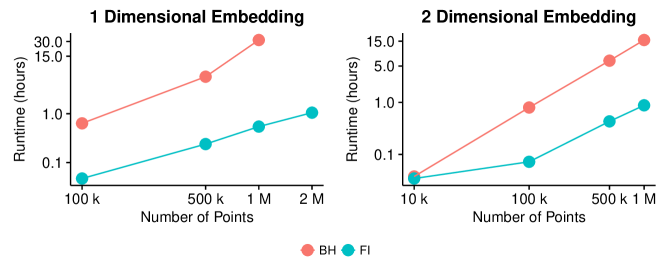
Figure 3. Time required to compute gradients for 1000 iterations of t-SNE using FFT-accelerated Interpolation-based (FI) t-SNE as compared to the Barnes-Hut (BH) t-SNE implementation.

3. The attractive forces $F_{\text{attr},i}$

At each step of gradient descent, the attractive forces on the $i$th point

$$F_{\text{attr},i}=\sum_{j\neq i}{p_{ij}q_{ij}Z(y_{i}-y_{j})}$$

attract it to other points in the embedding that are close in the original space. In practice, computing the interaction energies $p_{ij}$ between all pairs of points is too expensive and hence van der Maaten (2014) restricts to computing, for every point, only the interactions with the $k$ nearest neighbors. In that implementation, nearest neighbors are computed with vantage-point trees (Yianilos (1993)), which are highly effective in low dimensions, but are prohibitively expensive when embedding large, high dimensional datasets.

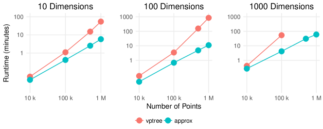
Figure 4. Computation of $p_{ij}$ in first phase of t-SNE

A recent theoretical advance by Linderman et al. (2017) can be used to optimize this step: it suggests that connecting every point to its (for example) $k=100$ nearest neighbors is not more effective than connecting every point to 2 randomly chosen points out of its 100 nearest neighbors. The main reason is that this randomized procedure, when executed on point clouds lying on manifolds, creates expander graphs at the local scale which represent the local geometry accurately at a slightly coarser level. In the purely discrete case, this relates to problems in random graphs first raised by Ulam and Erdős-Renyi, and we refer to Linderman et al. (2017) for details. This simple insight may allow for a massive speedup since the number of interaction terms $\#\left\{p_{ij}:p_{ij}\neq 0\right\}$ is much smaller. In practice, we use this result to justify the replacement of nearest neighbors with approximate nearest neighbors. Specifically, we compute approximate nearest neighbors using a randomized nearest neighbor method called ANNOY (Bernhardsson (2017)), as we expect the resulting “near neighbors” to capture the local geometry at least as effectively as the same number of nearest neighbors. We further accelerated this step by parallelizing the neighbor lookups. The resulting speed-ups over the vantage point tree approach for computing $F_{\text{attr},i}$ are shown in Fig. 4, as measured on a machine with 12 Intel Xeon E7540 CPUs clocked at 2.00GHz.

4. Early and Late Exaggeration

In the expression for the gradient descent, the sum of attractive and repulsive forces,

$$\frac{1}{4}\frac{\partial C}{\partial y_{i}}=\alpha\sum_{j\neq i}{p_{ij}q_{ij}Z(y_{i}-y_{j})}-\sum_{j\neq i}{q_{ij}^{2}Z(y_{i}-y_{j})},$$

the numerical quantity $\alpha>0$ plays a substantial role as it determines the strength of attraction between points that are similar (in the sense of pairs $x_{i},x_{j}$ with $p_{ij}$ large). In early exaggeration, first $\alpha=12$ for the first several hundred iterations, after which it set to $1$ (see van der Maaten and Hinton (2008)). One of the main results of Linderman and Steinerberger (2017) is that $\alpha$ plays a crucial role and that when it is set large enough, t-SNE is guaranteed to separate well-clustered data and also successfully embed various synthetic datasets (e.g. a swiss roll) that were previously thought to be poorly embedded by t-SNE.

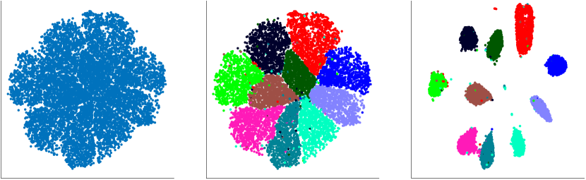
Figure 5. t-SNE embedding of 1 million digits from the Infinite MNIST dataset. Late exaggeration of $\alpha=12$ for the last 250 of the 1000 iterations (right) allows for clusters to be more easily distinguished than without it (left and middle).

We present a novel variation called “late exaggeration,” which refers to setting $\alpha>1$ for the last several hundred iterations. This approach seems to produce more easily interpretable visualizations: one recurring issue with t-SNE outputs (see Fig. 5) is that the arising structure, while clustered, has its clusters close to each other and does not allow for an easy identification of segments. By increasing $\alpha$ (and thus the attraction between points in the same cluster), the clusters contract and are more easily distinguishable.

5. t-SNE Heatmaps

The 2D t-SNE plot has become a staple of many scRNA-seq analyses, in which it is used to visualize clusters of cells, colored by the expression of interesting genes. Although this information is presented in 2D, users are most interested in which genes are associated with which clusters, not the 2D shape or relations of the clusters. In general, the location of clusters with respect to one another is meaningless, and their 2D shape is not interpretable and dependent on initialization (Wattenberg et al. (2016)). We hypothesize that 1D t-SNE would contain the same information as 2D t-SNE, and since it is much more compact, it would allow simultaneous visualization of the expression of hundreds of genes in a heatmap-like fashion. The general idea is shown in Fig. 6, where we embedded the 49k retinal cells of Macosko et al. (2015) using 1D and 2D t-SNE and assigned corresponding points the same color to show that the embeddings are equivalent.

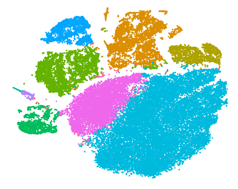
Figure 6. Left: 1D t-SNE of 49k retinal cells. The first three rows are colored by expression of three genes specific to individual clusters, and the fourth row is colored by clusters identified using dbscan. Uniform noise was added as a “Y-axis” of each row so that more cells would be visible. Right: 2D t-SNE plot colored by the clusters assigned using the 1D t-SNE, showing that 1D t-SNE contains generally the same information as 2D.

This 1D t-SNE representation can be extended into a visualization we call “t-SNE Heatmaps.” The 1D t-SNE is first discretized into $p$ bins, and we sum the expression of each gene in each of the bins, such that each gene $g$ is a vector in $\mathbb{R}^{p}$. A distance between genes is now defined as the Euclidean distance between these vectors. In practice, the user provides a set of genes of interest (GOI), and this gene set is then enriched with genes that are closest to the genes of interest in this metric. Each of the $p$-vectors corresponding to this new gene set are rows in a heatmap, and can be used to visualize hundreds of genes’ expression on the t-SNE embedding. We give a small example in Fig. 7, where three genes in corresponding to known Retinal subpopulations are enriched with the four genes closest to each in the t-SNE metric and visualized in this heatmap format.

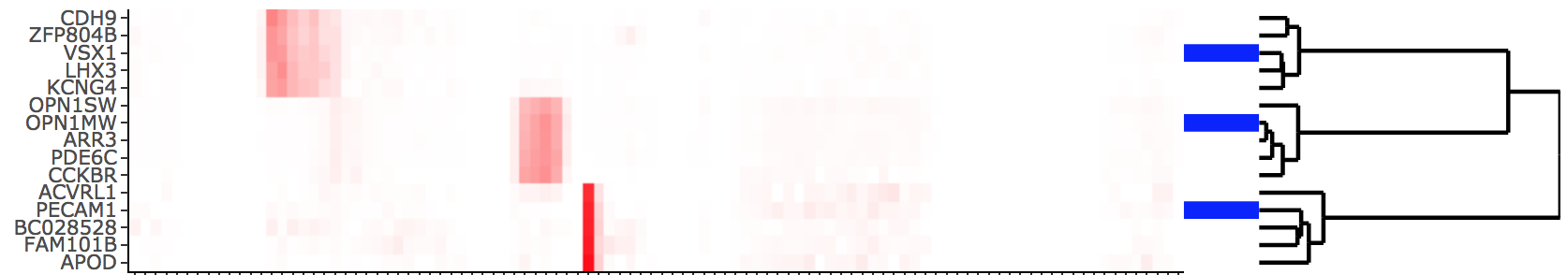
Figure 7. t-SNE heatmap using 1D embedding of Fig. 6.

In general, the rows need not correspond to individual genes; if a method for clustering genes is available, then t-SNE Heatmaps can be used to visualize how the cell clusters are associated with gene clusters. Overall, t-SNE Heatmaps uses the 1D t-SNE of the cells to define a distance on the genes, and could be similarly extended to define a distance on the cells. This would allow for t-SNE based iterative methods to be developed, similar to Mishne et al. (2017), where the the embedding of the cells is used to improve the embedding of the genes, which is then used to improve the embedding of the cells, and so forth.

6. Out-of-Core PCA

The methods for t-SNE presented above allow for embedding of millions of points in only hours, but can only be used to reduce the dimensionality of datasets that can fit in the memory. For many large, high dimensional datasets, specialized servers must be used in order to simply load the data. For instance, a single cell RNA-seq dataset with a million cells, where the expression of $20,000$ genes are measured for each cell, requires 160GB of memory - far exceeding the capacity of a standard personal computer. In order to allow for visualization and analysis of such datasets on resource-limited machines, we present an out-of-core implementation of randomized PCA, which can be used to compute the top few (e.g. 50) principal components of a dataset to high accuracy, without ever loading it in its entirety (Halko et al. (2011a)).

6.1. Randomized Methods for PCA

The goal of PCA is to approximate the matrix being analyzed (after mean centering of its columns) with a low-rank matrix. PCA is primarily useful when such an approximation makes sense; that is, when the matrix being analyzed is approximately low-rank. If the input matrix is low-rank, then by definition, its range is low-dimensional. As such, when the input matrix is applied to a small number of random vectors, the resulting vectors nearly span its range. This observation is the core idea behind randomized algorithms for PCA: applying the input matrix to a small number of random vectors results in vectors that approximate the range of the matrix. Then, simple linear algebra techniques can be used to compute the principal components. Notably, the only operations involving the large input matrix are matrix-vector multiplications, which are easily parallelized, and for which highly optimized implementations exist. Randomized algorithms have been rigorously proven to be remarkably accurate with extremely high probability (e.g. Halko et al. (2011b); Witten and Candes (2015)), because for a rank-$k$ matrix, as few as $l=k+2$ random vectors are sufficient for the probability of missing a significant part of the range to be negligible. The algorithm and its underlying theory are covered in detail in Halko et al. (2011b). An easy-to-use “black box” implementation of randomized PCA is available and described in Li et al. (2017), but it requires the entire matrix to be loaded in the memory. We present an out-of-core implementation of PCA in R, oocPCA, allowing for decomposition of matrices which cannot fit in the memory.

Input: Matrix $A$ of size $m\times n$ stored in slow memory, non-negative integers $its$, $k$, $l$, $b$, where $0<k\leq l<\min(m,n)$, and $l$ defaults to $k+2$

Output: Orthonormal $U$ of size $m\times k$, non-negative diagonal matrix $\Sigma$ of size $k\times k$, orthonormal $V$ of size $n\times k$, such that $A\approx U\Sigma V^{*}$

1

2Generate uniform random matrix $\Omega$ of size $n\times l$

3Form $Y_{0}=A\Omega$ block-wise, $b$ rows at a time

4Renormalize with LU factorization $L_{0}U_{0}=Y_{0}$

5for $i\leftarrow 1$ to $its$ do

6       Form $Y_{i}=AA^{*}L_{i-1}$ block-wise, $b$ rows at a time

7      if $i<its$ then

8             Renormalize with LU factorization $L_{i}U_{i}=Y_{i}$

9       end if

10      

11 end for

12

13Renormalize with QR factorization $QR=Y_{i}$

14Compute SVD of small matrix $U^{\prime}\Sigma V^{*}=Q^{*}A$

15Set $U=QU^{\prime}$

Algorithm 2 Out-of-Core PCA (oocPCA)

6.2. Implementation

Our implementation is described in Algorithm 1. Given an $m\times n$ matrix of doubles $A$, stored in row-major format on the disk of a machine with $M$ bytes of available memory, the number of rows that can fit in the memory is calculated as $b=\left\lfloor\frac{M}{8mn}\right\rfloor$. The only operations performed using $A$ are matrix multiplications, which can be performed block-wise. Specifically, the matrix product $AB$, where $B$ is an $n\times p$ matrix stored in the fast memory, can be computed by loading the first $b$ rows of $A$, and forming the inner product of each row with the columns of $B$. The process can be continued with the remaining blocks of the matrix, essentially “filling in” the product $AB$ with each new block. In this manner, left multiplication by $A$ can be computed without ever loading the full matrix $A$.

By simply replacing the matrix multiplications in Li et al. (2017)’s implementation with block-wise matrix multiplication, an out-of-core algorithm can be obtained. However, significant optimization is possible. The run-time of an out-of-core algorithm is almost entirely determined by disk access time; namely, the number of times the matrix must be loaded to the memory. As suggested in Li et al. (2017), the renormalization step between the application of $A$ and $A^{*}$ is not necessary in most cases, and in the out-of-core setting, doubles the number of times $A$ must be loaded per power iterations. In our implementation, we remove this renormalization step, and apply $AA^{*}$ simultaneously, hence requiring the matrix only be loaded once per iteration.

Our implementation is in C++ with an R (R Core Team (2017)) wrapper. For maximum optimization of linear algebra operations, we use the highly parallelized Intel MKL for all BLAS functions (e.g. matrix multiplications). The R wrapper provides functions for PCA of matrices in CSV and in binary format. Furthermore, basic preprocessing steps including $\log$ transformation and mean centering of rows and/or columns can also be performed prior to decomposition, so that the matrix need not ever be fully stored in the memory.

6.3. Experiments

Memory (GB)	1	2	8	32	128	300
Time (Min)	15.9	12.8	12.7	12.0	10.5	8.4

Figure 8. PCA of $$1,000,000$\times$30,000$$ rank-$50$ matrix with varying memory limitations

We generated a random $$1,000,000$\times$30,000$$ rank-$50$ matrix of doubles, which would require $240$GB to simply store in the memory, far exceeding the memory capacity of a personal computer. Using oocPCA we can compute the top principal components of the matrix with much less memory (Fig. 8). By storing only 1GB of the matrix in the memory at a time, and all other parameters set to default, the top $50$ principal components of this matrix can be computed in 16 minutes, while attaining an approximation accuracy of $\sim 10^{-9}$ in the spectral norm.

7. Summary and Discussion

In this work, we present an implementation of t-SNE that allows for embedding of high dimensional datasets with millions of points in only a few hours. Our implementation includes a “late exaggeration” feature, which can make it easier to identify clusters in t-SNE plots. Finally, we presented an out-of-core algorithm for PCA, allowing for analysis and visualization of datasets that cannot fit into the memory. A natural extension of the present work is the analysis of large scRNA-seq datasets, and we are currently applying this approach to analyze the 1.3 million mouse brain cells dataset of 10X Genomics (2016). Our methods allow for visualization of these datasets, without subsampling, on a standard personal computer in a reasonable amount of time.

8. Software Availability

FIt-SNE and ooPCA are both available at https://github.com/KlugerLab/. The FIt-SNE repository also contains a script for producing t-SNE Heatmap visualizations.

9. Acknowledgements

The authors would like to thank Vladimir Rokhlin and Mark Tygert for many useful discussions.

10. Appendix

In Section §2 we noted that the repulsive forces $F_{\text{rep},k}$ defined in eq. 1 can be expressed as $s+2$ sums of the form

$$\phi(y_{i})=\sum_{j=1}^{N}K(y_{i},y_{j})q_{j}$$

where the kernel $K(y,z)$ is either

$$K_{1}(y,z)=\frac{1}{(1+\|y-z\|^{2})}\,,\quad\text{or}\quad K_{2}(y,z)=\frac{1}{(1+\|y-z\|^{2})^{2}}\,,$$

for $y,z\in\mathbb{R}^{s}$. In this appendix, we demonstrate for $s=2$. The following $4$ sums are computed at each step of gradient descent:

$$h_{1,j} =\sum_{\begin{subarray}{c}\ell=1\\ \ell\neq j\end{subarray}}^{N}\frac{1}{(1+\|y_{\ell}-y_{j}\|^{2})}\,,$$

$$h_{2,k} =\sum_{\begin{subarray}{c}\ell=1\\ \ell\neq k\end{subarray}}^{N}\frac{y_{\ell}(1)}{\left(1+\|y_{\ell}-y_{k}\|^{2}\right)^{2}}\,,$$

$$h_{3,k} =\sum_{\begin{subarray}{c}\ell=1\\ \ell\neq k\end{subarray}}^{N}\frac{y_{\ell}(2)}{\left(1+\|y_{\ell}-y_{k}\|^{2}\right)^{2}}\,,$$

$$h_{4,k} =\sum_{\begin{subarray}{c}\ell=1\\ \ell\neq k\end{subarray}}^{N}\frac{1}{\left(1+\|y_{\ell}-y_{k}\|^{2}\right)^{2}}\,.$$

At each step of gradient descent, the repulsive forces can then be expressed in terms of these $4$ sums as follows:

$$F_{\text{rep},k}(1) =\left(\sum_{\begin{subarray}{c}\ell=1\\ \ell\neq k\end{subarray}}^{N}\frac{y_{\ell}(1)-y_{k}(1)}{\left(1+\|y_{\ell}-y_{k}\|^{2}\right)^{2}}\right)\Bigg{/}\left(\mathop{\sum_{\begin{subarray}{c}j=1\end{subarray}}^{N}\sum_{\begin{subarray}{c}\ell=1\end{subarray}}^{N}}_{\ell\neq j}\frac{1}{(1+\|y_{\ell}-y_{j}\|^{2})}\right)$$

$$=\left(h_{2,k}-y_{k}(1)h_{4,k}\right)/Z,$$

$$F_{\text{rep},k}(2) =\sum_{\begin{subarray}{c}\ell=0\\ \ell\neq k\end{subarray}}^{N}\frac{y_{\ell}(2)-y_{k}(2)}{\left(1+\|y_{\ell}-y_{k}\|^{2}\right)^{2}}\Bigg{/}\left(\mathop{\sum_{\begin{subarray}{c}j=1\end{subarray}}^{N}\sum_{\begin{subarray}{c}\ell=1\end{subarray}}^{N}}_{\ell\neq j}\frac{1}{(1+\|y_{\ell}-y_{j}\|^{2})}\right)$$

$$=\left(h_{3,k}-y_{k}(2)h_{4,k}\right)/Z,$$

where

$$Z =\sum_{\begin{subarray}{c}j=1\end{subarray}}^{N}h_{1,j}\,.$$

References

- 10X Genomics (2016) 10X Genomics (2016). Transciptional profiling of 1.3 million brain cells with the chromium single cell 3’ solution. Application Note.
- Barnes and Hut (1986) Barnes, J. and Hut, P. (1986). A hierarchical O(N log N) force-calculation algorithm. Nature, 324(6096):446–449.
- Bernhardsson (2017) Bernhardsson, E. (2017). Annoy: Approximate nearest neighbors in c++/python optimized for memory usage and loading/saving to disk. https://github.com/spotify/annoy.
- Halko et al. (2011a) Halko, N., Martinsson, P.-G., Shkolnisky, Y., and Tygert, M. (2011a). An algorithm for the principal component analysis of large data sets. SIAM Journal on Scientific computing, 33(5):2580–2594.
- Halko et al. (2011b) Halko, N., Martinsson, P.-G., and Tropp, J. A. (2011b). Finding structure with randomness: Probabilistic algorithms for constructing approximate matrix decompositions. SIAM Review, 53(2):217–288.
- Li et al. (2017) Li, H., Linderman, G. C., Szlam, A., Stanton, K. P., Kluger, Y., and Tygert, M. (2017). Algorithm 971: an implementation of a randomized algorithm for principal component analysis. ACM Transactions on Mathematical Software (TOMS), 43(3):28.
- Linderman et al. (2017) Linderman, G. C., Mishne, G., Kluger, Y., and Steinerberger, S. (2017). Randomized near neighbor graphs, giant components, and applications in data science. arXiv preprint arXiv:1711.04712.
- Linderman and Steinerberger (2017) Linderman, G. C. and Steinerberger, S. (2017). Clustering with t-SNE, provably. arXiv preprint arXiv:1706.02582.
- Macosko et al. (2015) Macosko, E. Z., Basu, A., Satija, R., Nemesh, J., Shekhar, K., Goldman, M., Tirosh, I., Bialas, A. R., Kamitaki, N., Martersteck, E. M., et al. (2015). Highly parallel genome-wide expression profiling of individual cells using nanoliter droplets. Cell, 161(5):1202–1214.
- Mishne et al. (2017) Mishne, G., Talmon, R., Cohen, I., Coifman, R. R., and Kluger, Y. (2017). Data-driven tree transforms and metrics. IEEE Transactions on Signal and Information Processing over Networks.
- R Core Team (2017) R Core Team (2017). R: A Language and Environment for Statistical Computing. R Foundation for Statistical Computing, Vienna, Austria.
- van der Maaten (2014) van der Maaten, L. (2014). Accelerating t-SNE using tree-based algorithms. Journal of machine learning research, 15(1):3221–3245.
- van der Maaten and Hinton (2008) van der Maaten, L. and Hinton, G. (2008). Visualizing data using t-SNE. Journal of Machine Learning Research, 9(Nov):2579–2605.
- Wattenberg et al. (2016) Wattenberg, M., Viégas, F., and Johnson, I. (2016). How to use t-SNE effectively. Distill, 1(10):e2.
- Witten and Candes (2015) Witten, R. and Candes, E. (2015). Randomized algorithms for low-rank matrix factorizations: sharp performance bounds. Algorithmica, 72(1):264–281.
- Yianilos (1993) Yianilos, P. N. (1993). Data structures and algorithms for nearest neighbor search in general metric spaces. In SODA, volume 93, pages 311–321.