Numerical study of blow-up mechanisms for Davey-Stewartson II systems

Abstract.

We present a detailed numerical study of various blow-up issues in the context of the focusing Davey-Stewartson II equation. To this end we study Gaussian initial data and perturbations of the lump and the explicit blow-up solution due to Ozawa. Based on the numerical results it is conjectured that the blow-up in all cases is self similar, and that the time dependent scaling is as in the Ozawa solution and not as in the stable blow-up of standard $L^{2}$ critical nonlinear Schrödinger equations. The blow-up profile is given by a dynamically rescaled lump.

1. Introduction

This paper is devoted to the study of blow-up mechanisms for solutions to the focusing Davey-Stewartson (DS) II equation

(1) $$\begin{array}[]{ccc}i\partial_{t}\psi+\partial_{xx}\psi-\partial_{yy}\psi-2\left(\Phi+\left|\psi\right|^{2}\right)\psi&=&0,\quad\psi:\mathbb{R}^{2}\times\mathbb{R}\to\mathbb{C},\\ \partial_{xx}\Phi+\partial_{yy}\Phi+2\partial_{xx}\left|\psi\right|^{2}&=&0,\quad\Phi:\mathbb{R}^{2}\times\mathbb{R}\to\mathbb{R},\\ \psi(.,0)=\psi_{0}.\end{array}$$

Equation (1) is a completely integrable [2, 38] two-dimensional nonlinear Schrödinger (NLS) equation which appeared first in the context of water waves ([10, 11, 3], see [26] for more references and a rigorous justification). It also appears in the context of ferromagnetism [27], plasma physics [31] and nonlinear optics [32]. Eliminating the mean field $\Phi$ from (1) by inverting the Laplace operator with some fall off condition at infinity, one gets as in [18]

(2) $$i\partial_{t}\psi+\Box\psi+2[(\Delta^{-1}\Box)|\psi|^{2}]\psi=0,$$

where $\Box=\partial_{xx}-\partial_{yy}$, and where $\Delta=\partial_{xx}+\partial_{yy}$ are the D’Alembert and Laplace operator respectively. The DS II equation can thus be seen as a nonlocal hyperbolic NLS equation.

The DS II equation as a special case of 2d NLS equations has a well known scaling invariance: if $\psi(x,y,t)$ is a solution to (1), so is $\lambda\psi(x/\lambda x,y/\lambda,t/\lambda^{2})$ with constant $\lambda\in\mathbb{R}/\{0\}$. Since the $L^{2}$ norm of $\psi$ is invariant under this rescaling, the equation is $L^{2}$ critical. It is well known that $L^{2}$ critical focusing NLS equations can have solutions with a blow-up in finite time, see [41] for a detailed discussion and for references. The above rescaling can be studied with a time dependent scaling factor $L(t)$ (which is not a symmetry of the equation),

(3) $$X=\frac{x}{L(t)},\quad Y=\frac{y}{L(t)},\quad\tau=\int_{0}^{t}\frac{dt^{\prime}}{L^{2}(t^{\prime})},\quad\Psi(\xi,\eta,\tau)=L(t)\psi(x,y,t).$$

It was shown by Merle and Raphaël [30] that in cases with a generic blow-up in one point, the blow-up of the NLS solution is self-similar and follows the ‘dynamical rescaling’ (3) with a scaling factor of the form

(4) $$L(t)\propto\sqrt{\frac{t~{}^{*}-t}{\ln|\ln(t^{*}-t)|}},$$

where $t^{*}$ is the blow-up time. If the spatial operators in (1) are both elliptic, the resulting equation is the elliptic-elliptic DS following the notation of [13]. Numerically its solutions appear to have finite time blow-up, see [35], but a proof for the blow-up mechanism as in [30] for the cubic NLS has not yet been established. On the other hand a global well posedness result for the hyperbolic NLS equation

$$i\partial_{t}\psi+\Box\psi+|\psi|^{2}\psi=0$$

appears to be given in [48]. Thus it is not obvious whether the focusing DS II equation should have solutions with a blow-up in finite time. But equation (1) has an additional symmetry sometimes referred to as pseudoconformal invariance: if $\psi(x,y,t)$ is a solution to the DS II equation for $t>0$, so is

(5) $$\tilde{\psi}(x,y,t)=\exp\left(\frac{i(x^{2}-y^{2})}{4t}\right)\psi\left(\frac{x}{t},\frac{y}{t},\frac{1}{t}\right).$$

This symmetry was used by Ozawa [34] to construct an exact blow-up solution starting from the lump solution (9) of the focusing DS II solution, a solitary wave solution with algebraic decay towards infinity. The blow-up in the Ozawa solution (10) is again self-similar, i.e., of the form (3), but this time with a scaling factor

(6) $$L(t)\propto t^{*}-t.$$

Note that a similar blow-up mechanism based on the pseudoconformal invariance is also known for the standard $L^{2}$ critical NLS equations, but that it is unstable in this case, see [30].

The question to be addressed numerically in this paper is whether the blow-up in DS II solutions observed in various examples is of the type (3), and if so whether it has the scaling (4) of the generic blow-up in NLS or the scaling (6) of the Ozawa solution, and what is the blow-up profile in this case. Numerical studies of blow-up in NLS equations allowed to give indications for analytical results in the field, see [41] for a detailed discussion and for references. First numerical studies of the DS II systems were presented in [49], the first study of blow-ups in DS II appeared in [7]. In [29] numerical experiments indicated that the lump soliton was unstable both against blow-up and being dispersed away (in dependence of whether the perturbed lump has a larger or smaller $L^{2}$ norm than the lump). These experiments were repeated with much higher resolution on parallel computers in [23]. There it was shown that the Ozawa solution is also unstable against being dispersed away or a blow-up before the blow-up time of the unperturbed solution. The mechanism of the latter, however, was not studied in [23]. In [18], this question was addressed in a similar way as blow-up in generalized Korteweg-de Vries (KdV) [16] and Kadomtsev-Petviashvili (KP) [17] equations. There certain norms of the solution were traced during the time evolution and matched to a dynamical rescaling (3) which allowed in [16, 17] to infer the scaling function $L(t)$ near blow-up. Since only serial computers were available in [18], the necessary resolution could not be reached in order to decide whether the blow-up is according to the scaling (4) or (6). It could be shown however that blow-up seems to be possible only in the integrable focusing DS II equation (1). In general DS II equations (a factor $\beta\in\mathbb{R}$ in front of the $\Phi$ in the first line of (1), see [13]), no blow-up was found in [18]. In [22] the so-called semiclassical limit for DS II equations was studied numerically. It was shown that blow-up appears only if the initial data are (locally near the maximum) symmetric with respect to the exchange of the spatial coordinates $x\mapsto y$, i.e., for instance in the radially symmetric case.

In the present article we study the cases with blow-up in [23] and [18] with a parallized code on GPUs. This allows to get the necessary resolution to identify the type of blow-up. Concretely we study perturbed lump solutions, a perturbed Ozawa solution, and Gaussian initial data. The results can be summarized in the following conjecture:

Conjecture 1.1.

Consider initial data $\psi_{0}\in C^{\infty}(\mathbb{R}^{2})\cap L^{2}(\mathbb{R}^{2})$ for the focusing DS II equation (1) with a single global maximum of $|\psi_{0}|$ such that the solution to DS II has a blow-up in finite time. Then the blow-up is self-similar according to (3) with a scaling factor $L(t)$ of the form (6) and the blow-up profile given by the lump, i.e.,

(7) $$\psi(x,y,t)=\frac{P(X,Y)}{L(t)}+\tilde{\psi},\quad P(X,Y)=\frac{2}{1+X^{2}+Y^{2}},\quad L(t)\sim t^{*}-t,$$

where $\tilde{\psi}$ is bounded for all $t$.

The paper is organized as follows: In section 2 we collect some known analytical facts on the focusing DS II equation. In section 3 we present the used numerical approaches and test them for the analytically known lump and for Ozawa’s blow-up solution. In section 4, we study the perturbed lump, a perturbed Ozawa solution, and Gaussian initial data. We add some concluding remarks in section 5.

2. Analytical preliminaries

In this section we review some known analytical facts on the DS II system which are relevant for the numerical studies to be presented in this paper.

For the Cauchy problem (1) based on a work by Fokas and Sung [12], Sung [42, 43, 44, 45] has proven the following

Theorem 2.1.

Let $\psi_{0}\in\mathcal{S}(\mathbb{R}^{2})$, the space of rapidly decreasing smooth functions. Then (1) possesses a unique global solution $\psi$ such that the mapping $t\mapsto\psi(\cdot,t)$ belongs to $C^{\infty}(\mathbb{R},\mathcal{S}(\mathbb{R}^{2}))$ if

$$||\widehat{\psi_{0}}||_{1}||\widehat{\psi_{0}}||_{\infty}<C,$$

where $C$ is an explicitly known constant.

Thus Sung obtains global well-posedness under the assumption that $\hat{\psi}_{0}\in L^{1}(\mathbb{R}^{2})\cap L^{\infty}(\mathbb{R}^{2})$ and $\psi_{0}\in L^{p}(\mathbb{R}^{2})$ for some $p\in[1,2),$ see [45]. Perry [36] has generalized this to the case of initial data in $H^{1,1}(\mathbb{R}^{2})=\{f\in L^{2}(\mathbb{R}^{2})\;\text{such that}\;\nabla f,(1+|\cdot|)f\in L^{2}(\mathbb{R}^{2})\}.$ Recently Nachman, Regev and Tataru [33] improved this to initial data $\psi_{0}\in L^{2}(\mathbb{R}^{2})$. Note that numerical results in [21, 18] indicate that the bound given in Theorem 2.1 is not optimal, i.e., that initial data not satisfying the condition can still lead to global existence in time of the solution.

The focusing DS II equation (1) is completely integrable and thus has an infinite number of conservation laws. The first two conserved quantities are the squared $L^{2}$ norm

$$||\psi||_{2}^{2}=\int_{\mathbb{R}^{2}}|\psi(x,y,t)|^{2}dxdy$$

and the energy (Hamiltonian)

(8) $$E(\psi(t))=\int_{\mathbb{R}^{2}}\left[|\partial_{x}\psi|^{2}-|\partial_{y}\psi|^{2}+(|\psi|^{2}+\Phi)|\psi|^{2})\right]dxdy.$$

The focusing DS II system possesses a family of localized solitary waves ([4, 1]) called lumps given by

(9) $$\psi(x,y,t)=2c\frac{\exp\left(-2i(\xi x-\eta y+2(\xi^{2}-\eta^{2})t)\right)}{|x+4\xi t+i(y+4\eta t)+z_{0}|^{2}+|c|^{2}}$$

where $(c,z_{0})\in\mathbb{C}^{2}$ and $(\xi,\eta)\in\mathbb{R}^{2}$ are constants. The lump moves with constant velocity $(-4\xi,-4\eta)$ and has an algebraic decay as $(x^{2}+y^{2})^{-1}$ for $x,y\to\infty$. We show the solution for $\xi=-1$, $\eta=0$, $z_{0}=0$, $c=1$ for various values of $t$ in Fig. 1.

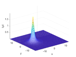
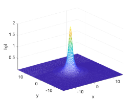
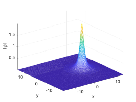
Figure 1. Lump solution (9) with parameters $\xi=-1$, $\eta=0$, $z_{0}=0$, $c=1$: On the left for $t=-1$, on the middle for $t=0$, and on the right for $t=1$.

Perry [37] showed that the lump is unstable in the inverse scattering picture in the sense that a small perturbation of lump initial data leads to an inverse scattering transform with different analytical properties than the lump. We address perturbations of the lump numerically in this paper.

Applying the pseudoconformal invariance (5) of DS II on the lump solution (9), Ozawa [34] has constructed an explicit blow-up solution to DS II.

Theorem 2.2 (Ozawa).

Let $a,b\in\mathbb{R}$ such that $ab<0$ and $t^{*}=-a/b$. Let

(10) $$\psi(x,y,t)=\exp\left(i\frac{b}{4(a+bt)}(x^{2}-y^{2})\right)\frac{v(X,Y)}{a+bt}$$

where

$$v(X,Y)=\frac{2}{1+X^{2}+Y^{2}},\,\,X=\frac{x}{a+bt},\,\,Y=\frac{y}{a+bt}.$$

Then, $\psi$ is a solution of (1) with

$$||\psi(t)||_{2}=||v||_{2}=2\sqrt{\pi}$$

and

$$|\psi(t)|^{2}\rightarrow 4\pi\delta\,\,\text{in}\quad\mathcal{S}^{\prime}\quad\mbox{when}\,\,t\rightarrow t^{*},$$

where $\delta$ is the Dirac measure, and where $\mathcal{S}^{\prime}$ is the space of tempered distributions.

The mass density $|\psi(.,t)|^{2}$ of the solution converges as $t\to t^{*}$ to a Dirac measure with total mass $||\psi(.,t)||^{2}_{2}=||\psi_{0}||^{2}_{2}$ . Every regularity breaks down at the blow-up point, but the solution continues to solve DS II for $t>t^{*}$. Note that the Ozawa solution is not in $H^{1}$. We show the real part of the solution for $a=1$ and $b=-4$ on the $x$-axis for different values of $t$ in Fig. 2. Note that the factor $\exp\left(i\frac{b}{4(a+bt)}(x^{2}-y^{2})\right)=\exp\left(-i(x^{2}-y^{2})/(t^{*}-t)\right)$ in (10) reads $\exp\left(i(X^{2}-Y^{2})/\tau\right)$ (for a proper choice of the integration constants). This means that the rapid oscillations will be suppressed near blow-up which is reached for $\tau\to\infty$. This behavior can be seen in Fig. 2, where the oscillations are most visible for $t=0$. Note the zoom in near blow-up in $x$ as well as the increasing amplitude near blow-up.

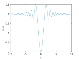
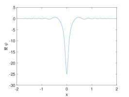
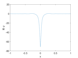
Figure 2. Real part of the Ozawa solution (10) for $a=1$, $b=-4$ on the $x$-axis for various values of $t$: On the left for $t=0$, on the middle for $t=0.23$ and on the right for $t=0.243$ close to the blow-up time $t^{*}=0.25$.

3. Numerical methods

In this section, we review the numerical methods for the study of blow-up in solutions to the focusing DS II equation (1). The approaches are tested via the propagation of lumps and the Ozawa solution.

3.1. Numerical methods for the time-evolution

In order to numerically integrate equation (1), we use a Fourier spectral method in the spatial coordinates. This means that the standard Fourier transform is approximated via a discrete Fourier transform which can be efficiently computed via the fast Fourier transform (FFT). In an abuse of notation we will use the same symbols for the continuous and the discrete Fourier transform. The discretization in Fourier space implies that (2) is approximated via a finite dimensional system of ordinary differential equations for the Fourier coefficients $\hat{\psi}=\mathcal{F}\psi$ of $\psi$ of the form

(11) $$\partial_{t}\widehat{\psi}=\mathcal{L}\widehat{\psi}+\mathcal{N}(\psi),$$

where $\mathcal{L}=-i(\xi_{1}^{2}-\xi_{2}^{2})$, and where $\mathcal{N}(\psi)=2i\mathcal{F}[\mathcal{F}^{-1}\{(\xi_{1}^{2}-\xi_{2}^{2})/(\xi_{1}^{2}+\xi_{2}^{2})\mathcal{F}(|\psi|^{2})\}\psi]$ denotes the nonlinearity; here $\xi_{1}$, $\xi_{2}$ are the dual Fourier variables for $x$ and $y$ respectively. For systems of the form (11) with diagonal $\mathcal{L}$ as in the case of Fourier methods, there are many efficient high-order time integrators, see [22] for a comparison of fourth order methods for DS II.

As in [23], we use here a fourth order splitting method. The motivation for these methods is the Trotter-Kato formula [47, 15]

$${\lim}_{n\rightarrow\infty}\left(e^{-tA/n}e^{-tB/n}\right)^{n}=e^{-t\left(A+B\right)},$$

where $A$ and $B$ are certain unbounded linear operators, for details see [15]. Splitting techniques have been studied by Bagrinovskii and Godunov in [6], by Strang [39], and for hyperbolic equations in Tappert [46] and Hardin and Tappert [14] (split step method for NLS).

For an equation of the form $u_{t}=\left(A+B\right)u$ the idea is to write the solution in the form

$$u(t)=\exp(c_{1}tA)\exp(d_{1}tB)\exp(c_{2}tA)\exp(d_{2}tB)\cdots\exp(c_{k}tA)\exp(d_{k}tB)u(0),$$

where the real numbers $(c_{1},\,\ldots,\,c_{k})$ and $(d_{1},\,\ldots,\,d_{k})$ represent fractional time steps. Yoshida [50] gave an approach which produces split step methods of any even order. Here the DS II equation (11) is split into

(12) $$\partial_{t}\hat{\psi}=-i(\xi_{1}^{2}-\xi_{2}^{2})\hat{\psi},$$

(13) $$\partial_{t}\hat{\psi}=2i\mathcal{F}\left[\mathcal{F}^{-1}\left\{\frac{\xi_{1}^{2}-\xi_{2}^{2}}{\xi_{1}^{2}+\xi_{2}^{2}}\mathcal{F}\left|\psi\right|^{2}\right\}\psi\right],$$

which are both explicitly integrable, the first one in Fourier space, the second in physical space since $|\psi|^{2}$ is constant in time for (13). Because of this property and the linearity of equation (12), the splitting scheme conserves the $L^{2}$ norm of $\psi$ which implies that the method is stable. But the conservation of the $L^{2}$ norm by the splitting scheme also has the consequence that the latter cannot be used to control the numerical accuracy. Instead we consider the numerically computed energy (8). It was shown in [22] that the quantity $\Delta_{E}=E(t)/E(0)-1$ can be used in this case to indicate the numerical accuracy which is overestimated by one to two orders of magnitude.

3.2. Singularity tracing and self-similar blow-up

It is well known that a (single) singularity $z_{0}\in\mathbb{C}$ of a function $f$ of the form $f(z)\sim(z-z_{0})^{\mu}$, with $\mu\not\in\mathbb{Z}$ implies the following asymptotic behavior for the corresponding Fourier transform

(14) $$|\widehat{f}(k)|\sim\frac{1}{k^{\mu+1}}e^{-k\delta},\quad|k|\gg 1,$$

where $\delta=\text{Im}\,z_{0}$. If numerically the Fourier transform is approached via an FFT, relation (14) can still be used to identify the type of the singularity via the quantity $\mu$ obtained by a fitting of the Fourier coefficients for large wave numbers to (14). This was first used in [40] to identify the appearance of a singularity.

In [20, 21] this approach was discussed with considerably higher resolution in detail and used to quantitatively identify the time where the distance $\delta$ of the singularity from the real axis becomes smaller than the minimal resolved distance via Fourier methods, i.e., $m:=2\pi D/N$ with $N\in\mathbb{N}$ being the number of Fourier modes and $2\pi D$ the length of the computational domain in physical space. A value of $\delta<m$ cannot be distinguished numerically from $0$.

Unfortunately this method is not applicable here for most of the studied examples because of the slow algebraic decrease of the lump and the Ozawa solution towards infinity. This implies that the approximation as a periodic function is as discussed not analytic on the domain boundaries. This leads already to an algebraic decrease of the Fourier coefficients, an effect which is not easily separated from the to be identified singularity in the complex plane. The Ozawa solution has the additional problem that it is rapidly oscillating which as discussed below leads also to oscillations in the Fourier coefficients. In addition the singularity tracing requires a very high resolution in time which is difficult to achieve in two-dimensional computations. Thus we proceed here as in [23] and stop the code once the computed energy indicates that the accuracy drops below plotting accuracy (typically if the quantity $\Delta_{E}<10^{-3}$).

The time at which the code is stopped because of the above criterion is obviously not the blow-up time itself. The latter will be identified by tracing the $L^{\infty}$ norm of the solution and matching it to what would be expected from a dynamical rescaling (3) of the DS II equation. Assuming that $L(t)$ vanishes at the blow-up, we can study the type of the blow-up for DS II in a similar way as it has been done for generalized KdV equations in [16], for generalized KP equations in [17] and for fractional NLS equations in [19]: we integrate DS II directly, as described above, and then we use some post-processing to characterize the type of blow-up via the rescaling (3). Since the $L^{2}$ norm of $\psi$ is invariant under this rescaling, we consider the $L^{\infty}$ norm of $\psi$. We get with (3) that

(15) $$||\psi(t,\cdot)||_{\infty}\propto\frac{1}{L}$$

for $t\to t^{*}$. Thus tracing the norm and matching it to a factor $(t^{*}-t)^{\gamma}$, it should be possible to determine both the blow-up time $t^{*}$ and the exponent $\gamma$. Concretely we trace the $L^{\infty}$ norm during the time evolution until the results as indicated by the energy conservation can no longer be trusted. Then we fit $||\psi||_{\infty}$, according to

(16) $$\ln||\psi||_{\infty}\sim\alpha+\gamma\ln(t^{*}-t),$$

for a certain number of the last recorded time steps before the code is stopped. The fitting is done with the optimization algorithm [25] distributed with Matlab to find constants $\alpha$, $\gamma$ and $t^{*}$ such that the residual of $\ln||\psi||_{\infty}-[\alpha+\gamma\ln(t^{*}-t)]$ becomes minimal. Note that it will be numerically impossible to distinguish the case $L(t)\propto\sqrt{t^{*}-t}$ from the formula (4) established analytically for $L^{2}$ critical NLS equations since the effect of the logarithms will be too small. Note also that the $L^{2}$ norm of $\psi_{x}$, which has been applied in [16] and [17] in a similar context, cannot be used in the case of the Ozawa solution for which the latter is not finite. Though here we approximate this solution via a periodic function for which all these norms are finite, the divergence of $||\psi_{x}||_{2}$ on the whole real line leads to numerical problems on the considered large computational domains. Therefore we only consider $||\psi||_{\infty}$ here.

The rescaling (3) implies for the equation (2)

(17) $$\begin{split}i\partial_{\tau}\Psi+(\partial_{X}^{2}-\partial_{Y}^{2})\Psi+i\partial_{\tau}(\ln L)(X\partial_{X}\Psi+Y\partial_{Y}\Psi+\Psi)+&\\ 2\left[(\partial_{X}^{2}+\partial_{Y}^{2})^{-1}(\partial_{X}^{2}-\partial_{Y}^{2}))|\Psi|^{2}\right]\Psi&=0.\end{split}$$

Whereas it is numerically inconvenient to solve this equation instead of DS for our examples (the lump and the Ozawa solution have algebraic decay towards infinity), it is interesting for theoretical reasons. In the limit $\tau\to\infty$, the blow-up is reached, and it is assumed that $\Psi$ is $\tau$ independent in the limit. If $L\propto t^{*}-t$ as for the Ozawa solution, also $\partial_{\tau}\ln L$ would vanish which leads for (17) to

(18) $$(\partial_{X}^{2}-\partial_{Y}^{2})\Psi+2\left[(\partial_{X}^{2}+\partial_{Y}^{2})^{-1}(\partial_{X}^{2}-\partial_{Y}^{2}))|\Psi|^{2}\right]\Psi=0.$$

The only known stationary, localized solution to this equation appears to be the lump though it is unclear whether it is the unique solution with this property. This would imply that a dynamically rescaled (according to (3)) lump could provide the blow-up profile for focusing DS II solutions.

3.3. Parallel computing on Graphic Processor Units

Since in the context of solutions of the focusing DS II equation strong gradients and rapid oscillations have to be resolved in two dimensions, the required high resolution cannot be reached by single thread codes. For this reason we use parallel computing in the form of heterogeneous computing with Graphics Processing Unit (GPUs). The code is implemented via NVIDIA’s CUDA C/C++ platform. Using CPU multithreading the parallelized stepper is run on the GPUs, whereas the control parameters such as the energy, $L^{2}$ norm etc. are concurrently computed on the CPU using the standard FFTW library, offloading computational duties from the GPUs.

The codes are run on a desktop computer equipped with two NVIDIA Quadro M5000s. The maximum resolution possible with the described hardware and all data used by the solver kept on the GPUs is $2^{14}\times 2^{14}$. All examples are run under the same scheme - first we do 2000 time steps to get close to the blow up point, followed by 2000 steps of size $\mathbb{d}t=10^{-5}$ (except in one case, as described below), that run through the blow up point. As already explained the code cannot be trusted after the distance between the pole in the complex plane and the real line becomes smaller than the spatial resolution or the conservation of the numerically computed energy drops below an acceptable threshold. Thus we perform exploratory low resolutions runs to establish roughly the blow-up time, and then apply the above approach for a high resolution analysis.

3.4. Tests

We test the numerical code on two examples. First, we propagate the analytically known lump solution, and then we simulate the Ozawa solution in order to test our approaches to identify blow-up.

3.4.1. Lump solution

We first test the lump solution (9). We use a domain with $D=50$ (we remind that the domain size is $2\pi D\times 2\pi D$) in order to handle the algebraic fall off and solution parameters $\xi=0$, $\eta=-1$, $z_{0}=0$, $c=1$, and $t\in[-6,6]$, i.e.,

$$\psi(x,y,-6)=2\frac{\exp(-2i(y+12))}{|x+i(y+24)|^{2}+1}$$

and propagate the solution to $t=6$ in $N_{t}=1000$ temporal steps, comparing it to the exact solution. The Fourier coefficients for the solution (at the final time, but the difference to the coefficients at the initial time is hardly visible) are shown on the right of Fig. 3. Due to the algebraic decay of the solution towards infinity, the solution is not analytical at the domain boundaries as a periodic function. This leads to the algebraic decay of the Fourier coefficients with the wave number $k$ for $|k|$ to infinity. The choice of the parameter $D$ in the computational domain $D[-\pi,\pi]\times D[-\pi,\pi]$ is motivated by exactly this decrease of the Fourier coefficients: for small values of $D$, the resolution is high in physical space, but the lack of analyticity leads to a slower decrease of the coefficients and thus of the numerical error. The latter problem is reduced for larger values of $D$, but then the number of points in the FFT per interval becomes smaller leading again to larger numerical errors. The used value $D=50$ is a compromise between these two effects.

The relative decrease of the Fourier coefficients by roughly 5 orders of magnitude (see Fig. 3 on the right) indicates that a numerical error of the order of $10^{-5}$ can be expected in this case. That this is indeed the case can be seen on the left of Fig. 3 where the $L^{\infty}$ norm of the difference between numerical and exact solution (normalized by the $L^{\infty}$ norm of the exact solution) can be seen in dependence of time. The computed relative energy is conserved to the order of $10^{-10}$. This shows that the problem is much better resolved in time than in space, the reason being as discussed the algebraic decay of the solution towards infinity.

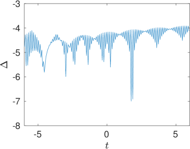
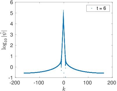
Figure 3. Propagation of the lump solution (9) with parameters $\xi=0$, $\eta=-1$, $z_{0}=0$, $c=1$: On the left the quantity $\Delta:=||\psi_{num}-\psi_{exact}||_{\infty}/||\psi_{exact}||_{\infty}$ indicating the numerical error, on the right the modulus of the Fourier coefficients on the $\xi_{1}$-axis at $t=6$. For the energy preservation we have $\max\Delta E=10^{-9.2994}$.

3.4.2. Ozawa solution

We consider the Ozawa solution (10) on a domain with $D=50$ with parameters $a=1$ and $b=-4$ having a blow-up at $t^{*}=0.25$ i.e., the situation shown in Fig. 2. For $t=0$ this leads to the initial condition

$$\psi(x,y,0)=2\frac{\exp(-i(x^{2}-y^{2}))}{1+x^{2}+y^{2}}.$$

The algebraic decay of the solution is clearly seen in the Fourier coefficients in Fig. 4, on the right for different times. The highly oscillatory character of the solution together with the algebraic decay already present for the lump makes these initial data especially challenging for the numerics. It can be seen that the oscillations in physical space lead together with the slow decay of the solution towards infinity to oscillations in coefficient space. Since the oscillations near blow-up are less important as discussed in the previous section, also the oscillations in coefficient space are reduced at later times.

It is well known (see already [7] and [23]) that splitting codes for DS will continue to run even after an analytical blow-up is encountered. This is different from generalized KdV codes where in general overflow errors lead to a stop of the code. However, some quantities show a jump at the numerically encountered blow-up. Since the split-step method preserves the $L^{2}$ norm exactly, the latter is essentially continuous there, but we see a jump in the energy in Fig. 4 on the left. We start our simulation at $t=0.21$ and execute 4000 steps with step size $\mathbb{d}t=10^{-5}$. The fitting of the Fourier coefficients shows that the critical distance is reached at $t=0.2430$ (step 3330). However, the energy preservation reaches the critical point $\Delta_{E}=10^{-4}$ before that, $t=0.2380$ at step 2980.

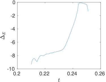
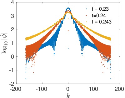
Figure 4. Modulus of the Fourier coefficients for the Ozawa solution with parameters $a=1$, $b=-4$ on the $\xi_{1}$-axis, for various values of $t$ on the right, and the corresponding relative computed energy $\Delta E$ on the left.

In Fig. 5 we show the $L^{\infty}$ norm of the solution on the left. Fitting this norm for the last 1000 time steps before losing resolution to formula (16), we get the blow-up time $t^{*}=0.2494$ and the blow-up rate of $\gamma=-0.9647$ as can be seen on the right of Fig. 5, both in excellent agreement with the analytic values $0.25$ and $-1$ respectively.

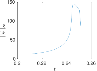
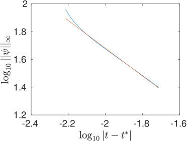
Figure 5. Numerically computed Ozawa solution with parameters $a=1$, $b=-4$, with blow-up time $t^{*}=0.25$ on a domain with $D=50$: on the left $||\psi||_{\infty}$ in dependence of time, on the right the $L^{\infty}$ norm for the last 1000 recorded time steps in a log-log plot together with a line with slope $-1$.

4. Numerical results

In this section we study blow-up in solutions to the focusing DS II equation (1) for various examples: two different instances of perturbed Ozawa initial data, perturbed lump initial data and Gaussian initial data in the so-called semi-classical regime. All examples except the Gaussian are computed on a domain with $D=50$, due to their algebraic fall off at infinity. For the Gaussian we use $D=2$, as the exponential fall off allows the solution to be well resolved on a much smaller domain. The results of this section are summarized in Conjecture 1.1.

4.1. Ozawa Solution deformed by a small Gaussian

We consider Ozawa initial data with parameters $a=1$ and $b=-4$, and deform it by adding a Gaussian centered at the origin of the coordinate system

$$\psi(x,y,0)=2\frac{\exp(-i(x^{2}-y^{2}))}{1+x^{2}+y^{2}}+0.1\exp{(-x^{2}-y^{2})}.$$

The computation is run for 2000 steps to time $0.225$ and then for another 2000 steps with step size $\mathbb{d}t=10^{-5}$. The relative computed energy $\Delta_{E}$ shown on the left of Fig. 6 has a jump at $t\approx 0.2326$ (step 2760) which indicates a loss of resolution in time. Therefore data for $t>0.2326$ will not be considered in the following though the Fourier coefficients shown in Fig. 6 on the right still indicate a relative spatial resolution of better than plotting accuracy. A fitting of the Fourier coefficients according to formula (14) indicates an approaching of the singularity in the complex plane only at a later time. This means that we run in this case first out of resolution in time before losing resolution in the spatial coordinates when approaching the blow-up.

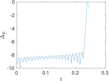
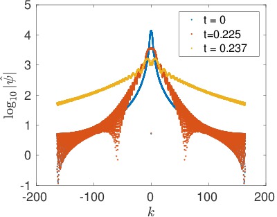
Figure 6. Solution to the DS II equation for Ozawa initial data deformed by a small Gaussian $0.1\exp(-x^{2}-y^{2})$: on the left the relative computed energy $\Delta E$, on the right the modulus of the Fourier coefficients on the $\xi_{1}$-axis at three different times.

The $L^{\infty}$ norm of the solution shown in Fig. 7 on the left indicates a blow-up before the blow-up time of the unperturbed Ozawa solution. Fitting the $L^{\infty}$ norm for the last 1000 recorded time steps to relation (16) assuming a self similar blow-up provides a blow-up time $t^{*}=0.2425$ and a blow-up rate $\gamma=-0.9570$ with a fitting residual 0.0033, see Fig. 7 on the right. Thus we get as in the case of the unperturbed Ozawa solution a blow-up rate proportional to $t^{*}-t$.

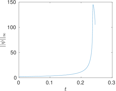
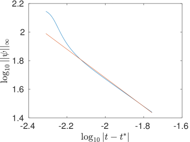
Figure 7. Solution to the DS II equation for Ozawa initial data deformed by a small Gaussian $0.1\exp(-x^{2}-y^{2})$: on the left the $L^{\infty}$ norm in dependence of time, on the right a log-log plot of the $L^{\infty}$ norm of the solution near the blow-up together with a straight line with slope $-1$.

The blow-up profile at the last recorded time is presented in Fig. 8 on the left. It appears to be locally radially symmetric and resembles a lump. Subtracting a lump rescaled according to (7) ($L$ is just determined via the maximum of the solution), we get the figure shown on the right of Fig. 8. It can be seen that the residual is more than an order of magnitude smaller than the maximum of the solution at this time. This gives a remarkable agreement with the conjectured blow-up profile (7) given that it is obtained at a time considerably smaller than the actual blow-up time.

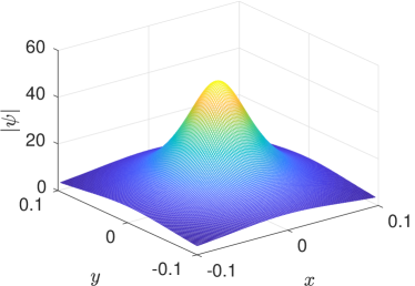
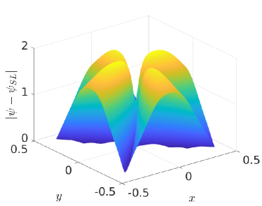
Figure 8. Solution to the DS II equation for Ozawa initial data deformed by a Gaussian $0.1\exp(-x^{2}-y^{2})$: blow-up profile at $t=0.2326$ on the left and the difference with a rescaled lump (according to (7)) on the right.

4.2. Ozawa initial data perturbed by a large Gaussian

We consider once more Ozawa initial data with parameters $a=1$ and $b=-4$, but deform it this time by adding a larger Gaussian centered at the origin of the coordinate system

$$\psi(x,y,0)=2\frac{\exp(-i(x^{2}-y^{2}))}{1+x^{2}+y^{2}}+0.5\exp{(-x^{2}-y^{2})}.$$

The code is run for 2000 time steps to $t=0.19$, followed by 2000 time steps $\mathrm{d}t=10^{-5}$. The computed relative energy in Fig. 9 on the left indicates a loss of resolution in time at $t\approx 0.2006$ (step $3060$). In Fig. 9 on the right, it can be seen that the Fourier coefficients at this time still indicate a spatial resolution to better than plotting accuracy. Thus once more, we run out of resolution in time first despite a very small time step near the blow-up.

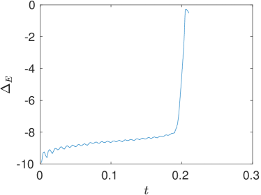
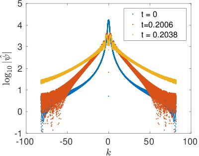
Figure 9. Solution to the DS II equation for Ozawa initial data deformed by a Gaussian $0.5\exp(-x^{2}-y^{2})$: on the left the relative computed energy $\Delta E$, on the right the modulus of the Fourier coefficients on the $\xi_{1}$-axis at three different times.

As shown in Fig. 10 on the left, the $L^{\infty}$ norm of the solution indicates a blow-up at an even earlier time than in Fig. 6. A fitting of the $L^{\infty}$ norm near blow-up according to 16 yields a blow-up time $t^{*}=0.2093$ and a blow-up rate $\gamma=-0.9487$ with residual $0.0043$, i.e., again the same rate as in the Ozawa solution.

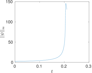
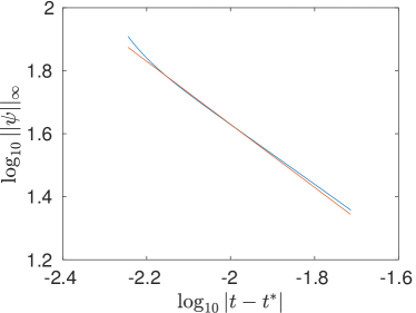
Figure 10. Solution to the DS II equation for Ozawa initial data deformed by a Gaussian $0.5\exp(-x^{2}-y^{2})$: on the left the $L^{\infty}$ norm in dependence of time, on the right a log-log plot of the $L^{\infty}$ norm of the solution near the blow-up together with a straight line with slope $-1$.

The blow-up profile at the last recorded time is presented in Fig. 11 on the left. Once more it seems to be radially symmetric in the vicinity of the maximum. We show the solution here on larger scales than in Fig. 8 to allow an overview of the solution, a close-up would look as in Fig. 8. If we subtract as there a lump rescaled according to (7), we get the figure shown on the right of Fig. 11. Once more the residual is more than an order of magnitude smaller than the maximum of the solution at this time, which shows an excellent agreement with the asymptotic blow-up profile.

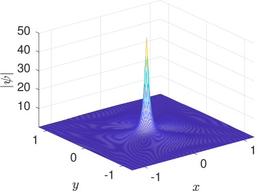
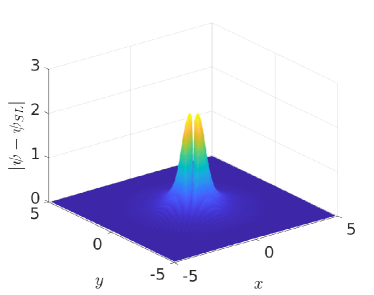
Figure 11. Solution to the DS II equation for Ozawa initial data deformed by a Gaussian $0.5\exp(-x^{2}-y^{2})$: blow-up profile at $t=0.2006$ on the left and the difference with a rescaled lump (according to (7)) on the right.

4.3. Perturbed lump solution

We consider lump initial data and multiply it by a factor $1.1$, i.e., we take the initial condition

$$\psi(x,y,0)=\frac{2.2}{1+x^{2}+y^{2}}.$$

The code is run for 2000 steps to $t=1.9$, followed by 2000 time steps $\mathrm{d}t=10^{-4}$. The time step $\mathrm{d}t$ is chosen so that $\mathrm{d}t/t^{*}$ is of the same order of magnitude in all experiments. A jump in the energy for $t\sim 2$ as shown in Fig. 12 on the left indicates again a loss of resolution in $t$, whereas the Fourier coefficients on the right of Fig. 12 also degrade for $t\sim 2$, again slightly later than the time where the energy has a jump.

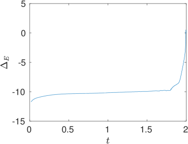
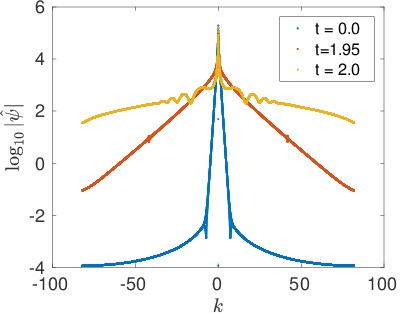
Figure 12. Solution to the focusing DS II equation for deformed lump initial data $\psi(x,y,0)=2.2/(1+x^{2}+y^{2})$: on the left the relative computed energy $\Delta E$, on the right the modulus of the Fourier coefficients on the $\xi_{1}$-axis at three different times.

The $L^{\infty}$ norm of the solution in Fig. 13 on the left is once more indicating a blow-up for $t>2$. The fit of the $L^{\infty}$ norm for the last 1000 time steps to (16) yields a blow-up time $t^{*}=2.066$ with blow-up rate $\gamma=-0.9733$ with a residual of 0.0043 as can be seen on the right of Fig. 13.

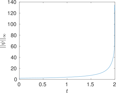
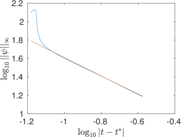
Figure 13. Solution to the focusing DS II equation for deformed lump initial data $\psi(x,y,0)=2.2/(1+x^{2}+y^{2})$: on the left the $L^{\infty}$ norm in dependence of time, on the right a log-log plot of the $L^{\infty}$ norm of the solution near the blow-up together with a straight line with slope $-1$.

The blow-up profile for $t=2$ can be seen in Fig. 14 on the left. Here the agreement with a dynamically rescaled lump (7) is even more striking than in the Ozawa examples above. As can be seen on the right of Fig. 14, the residual of the numerical solution and the rescaled lump is almost two orders of magnitude smaller than the maximum of the solution.

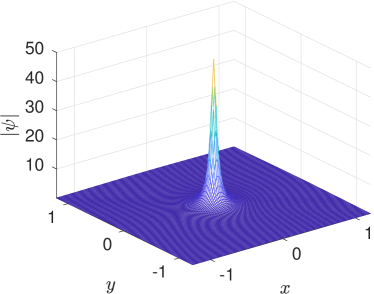
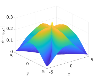
Figure 14. Solution to the focusing DS II equation for deformed lump initial data $\psi(x,y,0)=2.2/(1+x^{2}+y^{2})$: blow-up profile at $t=1.983$ on the left and the difference with a rescaled lump (according to (7)) on the right.

4.4. Gaussian initial data

If one is interested in the solution to the DS II equation for localized initial data varying on length scales of order $1/\epsilon$, and this for times of order $1/\epsilon$ with $\epsilon\ll 1$, a way to treat this is a change of coordinates $x\mapsto\epsilon x$, $y\mapsto\epsilon y$, and $t\mapsto\epsilon t$. This leads for (1) to the equation (in an abuse of notation we use the same symbols as before)

(19) $$\begin{array}[]{ccc}i\epsilon\partial_{t}\psi+\epsilon^{2}\partial_{xx}\psi-\epsilon^{2}\partial_{yy}\psi-2\left(\Phi+\left|\psi\right|^{2}\right)\psi&=&0,\\ \partial_{xx}\Phi+\partial_{yy}\Phi+2\partial_{xx}\left|\psi\right|^{2}&=&0.\end{array}$$

Thus it is possible to consider a family of equations (depending on the parameter $\epsilon$) for $\epsilon$-dependent initial data, which allows to study the semiclassical limit of DS II, see for instance [21, 5].

For equation (19) with $\epsilon=0.1$, we consider Gaussian initial data

$$\psi(x,y,0)=\exp(-x^{2}-y^{2})$$

on a domain with $D=2$. The computed energy jumps at $t=0.2954$ (step 3540), whereas the fitting of the Fourier coefficients according to (14) indicates a singularity at a distance from the real axis smaller than the spatial resolution at $t=0.2956$ (step 3557). Thus the loss of resolution in time and in space happens at roughly the same time in this example.

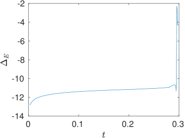
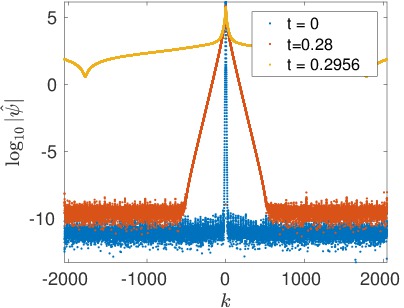
Figure 15. Solution to the focusing DS II equation (19) for Gaussian initial data initial data $\psi(x,y,0)=\exp(-x^{2}-y^{2})$ and $\epsilon=0.1$: on the left the relative computed energy $\Delta E$, on the right the modulus of the Fourier coefficients on the $\xi_{1}$-axis at three different times.

The $L^{\infty}$ norm on the left of Fig. 16 indicates a rapid blow-up. Fitting the norm according to (16) gives a blow-up time $t^{*}=0.2965$ and a blow-up rate $\gamma=-0.9278$. In this case, due to the exponential decay of the solution in the spatial directions we are able to use a much smaller computational domain and thus to work with a much higher spatial resolution as before. This allowed to get much closer to the actual blow-up time than in the algebraically decaying examples above.

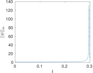
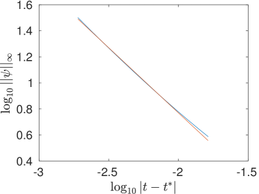
Figure 16. Solution to the focusing DS II equation (19) for Gaussian initial data initial data $\psi(x,y,0)=\exp(-x^{2}-y^{2})$ and $\epsilon=0.1$: on the left the $L^{\infty}$ norm in dependence of time, on the right a log-log plot of the $L^{\infty}$ norm of the solution near the blow-up together with a straight line with slope $-1$.

The blow-up profile can be seen in Fig. 17 on the left. Subtracting a rescaled lump (according to (7), we obtain the residual on the right of the same figure. This indicates that also in this case, the blow-up profile appears to be given by a dynamically rescaled lump.

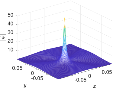
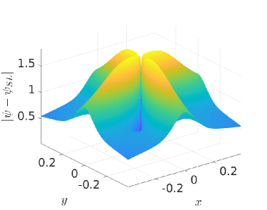
Figure 17. Solution to the focusing DS II equation (19) for Gaussian initial data initial data $\psi(x,y,0)=\exp(-x^{2}-y^{2})$ and $\epsilon=0.1$: blow-up profile at $t=0.2950$ on the left and the difference with a rescaled lump (according to (7)) on the right.

5. Outlook

In this paper we have studied blow-up phenomena in the focusing DS II equation for asymptotically localized initial data with a single maximum of the modulus. It was shown that initial data both with algebraic and with exponential decay can lead to a blow-up if the $L^{\infty}$ norm of the initial data is sufficiently large. Already in [20] and [18] it was shown that blow-up occurs only if the initial data are locally radially symmetric near the maximum. It would be interesting to study this symmetry question in more detail since it appears to be related to the lump appearing as a blow-up profile in a self-similar blow-up. This question would be in particular intriguing in the context of several humps which could blow up at the same time if the initial data are carefully chosen.

To study such questions, higher resolution than available for the present study will be needed. A possible way to address this would be to take a multi-domain spectral approach as in [8] and references therein which would be especially beneficial in the case of an algebraic decay of the solution towards infinity. It would also allow to allocate more resolution near a blow-up by introducing adapted domains. In contrast to [8] where a Laplace operator in the NLS equation was studied, DS II equations have a d’Alembert operator for which a different compactification at infinity will have to be introduced. This is will be the topic of future work.

Acknowledgements.

This work was partially supported by the program PARI and the FEDER 2016 and 2017. We thank J.-C. Saut for helpful discussions and hints.

References

- [1] M.J. Ablowitz and P.A. Clarkson, Solitons, nonlinear evolution equations and inverse scattering, London Mathematical Society Lecture Notes series 149, Cambridge University Press, (1991).
- [2] M. Ablowitz and R. Haberman. Nonlinear evolution equations in two and three dimensions. Phys. Rev. Lett., 35:11858, 1975.
- [3] M.J. Ablowitz and H. Segur, On the evolution of packets of water waves, J. Fluid Mech. 92 (1979), 691-715.
- [4] V.A. Arkadiev, A.K. Pogrebkov and M.C. Polivanov, Inverse scattering transform and soliton solution for Davey-Stewartson II equation, Physica D 36 (1089), 188-197.
- [5] O. Assainova, C. Klein, K. McLaughlin and P. Miller, A Study of the Direct Spectral Transform for the Defocusing Davey-Stewartson II Equation in the Semiclassical Limit, http://arxiv.org/abs/1710.03429
- [6] K. A. Bagrinovskii and S. Godunov, Difference Schemes for multi-dimensional Problems, Dokl.Acad. Nauk., 115 (1957), pp. 431433.
- [7] C. Besse, N. Mauser and H.-P. Stimming, Numerical study of the Davey-Stewartson system, M2AN Math. Model. Numer. Anal., 38, (6) (2004), 1035-1054.
- [8] M. Birem and C. Klein, Multidomain spectral method for Schrödinger equations, Adv. Comp. Math., 42(2), 395-423 DOI 10.1007/s10444-015-9429-9 (2016).
- [9] R. Cipolatti, On the instability of ground states for a Davey-Stewartson system, Ann.Inst. H. Poincaré, Phys.Théor. 58 (1993), 85-104.
- [10] A. Davey and K. Stewartson, One three-dimensional packets of water waves, Proc. Roy. Soc. Lond. A 338 (1974), 101-110.
- [11] V.D. Djordjevic and L.G. Redekopp, On two-dimensional packets of capillary-gravity waves, J. Fluid Mech. 79 (1977), 703-714.
- [12] A. Fokas, L.Y. Sung, On the solvability of the N-wave, Davey-Stewartson and Kadomtsev-Petviashvili equations, Inv. probl. 8(5), (1992) 673-708
- [13] J.-M. Ghidaglia and J.-C. Saut, On the initial value problem for the Davey-Stewartson systems, Nonlinearity, 3, (1990), 475-506.
- [14] R. H. Hardin and F. D. Tappert, Applications of the Split-Step Fourier Method to the numerical Solution of nonlinear and variable Coefficient Wave Equations, SIAM Rev., 15 (1973), p. 423.
- [15] T. Kato, Trotter product formula for an arbitrary pair of self-adjoint contraction semi- groups, vol. 3, Academic Press, Boston, 1978, pp. 185-195.
- [16] C. Klein and R. Peter, Numerical study of blow-up in solutions to generalized Korteweg-de Vries equations, Physica D 304-305 (2015), 52-78 DOI 10.1016/j.physd.2015.04.003.
- [17] C. Klein and R. Peter, Numerical study of blow-up in solutions to generalized Kadomtsev-Petviashvili equations, Discr. Cont. Dyn. Syst. B 19(6), (2014) doi:10.3934/dcdsb.2014.19.1689
- [18] C. Klein and J.-C. Saut, A numerical approach to Blow-up issues for Davey-Stewartson II type systems, Comm. Pure Appl. Anal. 14:4, 1443–1467 (2015)
- [19] C. Klein, C. Sparber and P. Markowich, Numerical study of fractional Nonlinear Schrödinger equations, Proc. R. Soc. A 470: (2014) DOI: 10.1098/rspa.2014.0364.
- [20] C. Klein and K. Roidot, Numerical study of shock formation in the dispersionless Kadomtsev-Petviashvili equation and dispersive regularizations. Phys. D 265 (2013), 1–25.
- [21] C. Klein and K. Roidot, Numerical Study of the semiclassical limit of the Davey-Stewartson II equations, Nonlinearity 27, 2177-2214 (2014).
- [22] C. Klein and K. Roidot, Fourth order time-stepping for Kadomtsev-Petviashvili and Davey-Stewartson equations, SIAM Journal on Scientific Computing Vol. 33, No. 6, DOI: 10.1137/100816663 (2011).
- [23] C. Klein, B. Muite and K. Roidot, Numerical Study of Blowup in the Davey-Stewartson System, Discr. Cont. Dyn. Syst. B, Vol. 18, No. 5, 1361–1387 (2013).
- [24] C. Klein, Fourth order time-stepping for low dispersion Korteweg-de Vries and nonlinear Schrödinger equation, ETNA Vol. 29 116-135 (2008).
- [25] J. C. Lagarias, J. A. Reeds, M. H. Wright, and P. E. Wright, Convergence properties of the Nelder-Mead simplex method in low dimensions. SIAM J. Optimization 9 (1998), 112–147.
- [26] D. Lannes, Water waves: mathematical theory and asymptotics, Mathematical Surveys and Monographs, vol 188 (2013), AMS, Providence.
- [27] H. Leblond, Electromagnetic waves in ferromagnets, J. Phys. A 32 (45) (1999), 7907-7932.
- [28] F. Linares and G. Ponce, On the Davey-Stewartson systems, Ann. Inst. H. Poincaré Anal. Non Linéaire, 10 (1993), 523-548.
- [29] M. McConnell, A. Fokas, and B. Pelloni, Localised coherent Solutions of the DSI and DSII Equations a numerical Study, Mathematics and Computers in Simulation, 69 (2005), 424-438.
- [30] F. Merle and P. Raphaël, The blow-up dynamic and upper bound rate for critical nonlinear Schrödinger equation, Ann. of Math (2) 161 (1) (2005), 157-222.
- [31] S.L. Musher, A.M. Rubenchik and V.E. Zakharov, Hamiltonian approach to the description of nonlinear plasma phenomena, Phys. Rep. 129 (5) (1985), 285-366.
- [32] A. Newell and J.V. Moloney, Nonlinear Optics, Addison-Wesley (1992).
- [33] A. I. Nachman, I. Regev, and D. I. Tataru, ÒA nonlinear Plancherel theorem with applications to global well-posedness for the defocusing Davey-Stewartson equation and to the inverse boundary value problem of Calderon, arXiv:1708.04759, 2017.
- [34] T. Ozawa, Exact blow-up solutions to the Cauchy problem for the Davey-Stewartson systems, Proc.Roy. Soc. London A, 436 (1992), 345-349.
- [35] G. Papanicolaou, C. Sulem, P.-L. Sulem and X.P. Wang, The focusing singularity of the Davey-Stewartson equations for gravity-capillary waves, Physica D 72 (1994), 61-86.
- [36] P.A. Perry, Global well-posedness and long time asymptotics for the defocussing Davey-Stewartson II equation in , With an appendix by Michael Christ. J. Spectral Theory 6 (2016), no. 3, 429Ð481.
- [37] P.A. Perry, Soliton Solutions and their (In)stability for the Focusing Davey-Stewartson II Equation, preprint arXiv:1611.00215, (2016).
- [38] E.I. Schulman, On the integrability of equations of Davey-Stewartson type, Theor. Math. Phys. 56 (1983), 131-136.
- [39] G. Strang, On the Construction and Comparison of Difference Schemes, SIAM J. Numer. Anal., 5 (1968), pp. 506-517.
- [40] C. Sulem, P.-L. Sulem, and H. Frisch, Tracing complex singularities with spectral methods, J. Comp. Phys., 50 (1983), pp. 138–161.
- [41] C. Sulem and P.-L.Sulem, The nonlinear Schrödinger equation: Self-Focusing and Wave Collapse. Springer Series in Mathematical Sciences Vol. 139, Springer Verlag 1999.
- [42] L.Y. Sung, An inverse scattering transform for the Davey-Stewartson equations. I, J. Math. Anal. Appl. 183 (1) (1994), 121-154.
- [43] L.Y. Sung, An inverse scattering transform for the Davey-Stewartson equations. II, J. Math. Anal. Appl. 183 (2) (1994), 289-325.
- [44] L.Y. Sung, An inverse scattering transform for the Davey-Stewartson equations. III, J. Math. Anal. Appl. 183 (3) (1994), 477-494.
- [45] L.-Y. Sung, Long-Time Decay of the Solutions of the Davey-Stewartson II Equations, J. Nonl. Sci., 5 (1995), pp. 433-452.
- [46] F. Tappert, Numerical Solutions of the Korteweg-de Vries Equation and its Generalizations by the Split-Step Fourier Method, Lectures in Applied Mathematics, 15 (1974), pp. 215-216.
- [47] H. Trotter, On the Product of Semi-Groups of Operators, Proceedings of the American Mathematical Society, 10 (1959), pp. 545-551.
- [48] N. Totz, Global well-posedness of 2D non-focusing Schrödinger equations via rigorous modulation approximation, J. Differential Equations 261 (2016) 2251-2299
- [49] P. White and J. Weideman, Numerical Simulation of Solitons and Dromions in the Davey- Stewartson System, Math. Comput. Simul., 37 (1994), pp. 469-479.
- [50] H. Yoshida, Construction of higher Order symplectic Integrators, Physics Letters A, 150 (1990), pp. 262-268 .