Hierarchy of Information Scrambling,
Thermalization, and Hydrodynamic Flow in Graphene

Abstract

We determine the information scrambling rate $\lambda_{L}$ due to electron-electron Coulomb interaction in graphene. $\lambda_{L}$ characterizes the growth of chaos and has been argued to give information about the thermalization and hydrodynamic transport coefficients of a many-body system. We demonstrate that $\lambda_{L}$ behaves for strong coupling similar to transport and energy relaxation rates. A weak coupling analysis, however, reveals that scrambling is related to dephasing or single particle relaxation. Furthermore, $\lambda_{L}$ is found to be parametrically larger than the collision rate relevant for hydrodynamic processes, such as electrical conduction or viscous flow, and the rate of energy relaxation, relevant for thermalization. Thus, while scrambling is obviously necessary for thermalization and quantum transport, it does generically not set the time scale for these processes. In addition we derive a quantum kinetic theory for information scrambling that resembles the celebrated Boltzmann equation and offers a physically transparent insight into quantum chaos in many-body systems.

The emergence of chaos is the most plausible explanation for the thermalization of closed quantum many-body systems. An efficient concept to quantify quantum chaos is through the scrambling rate $\lambda_{L}$ Larkin1969 ; Sekino2008 . After the time $\lambda_{L}^{-1}$ of the evolution of an out-of-equilibrium initial state, quantum entanglement has spread across the system. Then, the initial state cannot be recovered, i.e. unscrambled, via local measurements. The system has lost its memory, a key prerequisite for thermalization. Still, it is unclear whether the scrambling rate is indeed the characteristic scale that determines the return to thermal equilibrium. Similar to the scrambling rate with respect to temporal evolution, the butterfly velocity $v_{B}$ characterizes the corresponding spread of entanglement in space after a local perturbation. Formally, these quantities can be determined from the growth in time or space of commutators or anticommutators of local operators $A$ and $B$,

$$\big{\langle}\left|\left[A\left(\mathbf{x},t\right),B\left(\mathbf{0},0\right)\right]\right|^{2}\big{\rangle}\sim e^{2\lambda_{L}\left(t-\frac{|\mathbf{x}|}{v_{B}}\right)}.$$ (1)

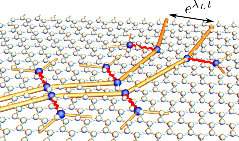
Figure 1: Exponentially diverging electron trajectories (orange) in graphene resulting from Coulomb interaction (red).

A transparent interpretation of this squared commutator exists in the quasi-classical limit for the motion of a particle with initial coordinate $q\left(0\right)$ and conjugate momentum $p\left(t\right)$ for which $\langle[p\left(t\right),p\left(0\right)]^{2}\rangle=\langle\big{(}\frac{\partial p\left(t\right)}{\partial q\left(0\right)}\big{)}^{2}\rangle$Larkin1969 . Exponential growth behavior of this correlator is e.g. realized by electrons in a weakly disordered metal Syzranov17 . Thus, the expectation value measures the dependence of the momentum at time $t$ as one changes the initial coordinates, a key measure for chaotic motion. The square in the commutator ensures that positive and negative momenta at time $t$ do not average to zero. The corresponding spread of an initial state of two nearby electrons in graphene is sketched in Fig. 1.

While the formal interpretation of scrambling is established in the information theoretic sense, with key applications in quantum circuits Hayden2007 , it is not obvious how to measure $\lambda_{L}$ or $v_{B}$ for a generic solid-state system. In fact it is unclear which specific physical observable might essentially probe these quantities and how this relates to thermalization. For example a close link to transport quantities was proposed and $v_{B}^{2}/\lambda_{L}$ related to the charge Blake2016 ; Blake2016_2 or heat Patel2017 diffusivities. The relation between scrambling and transport seems consistent with the bound on chaos $\lambda_{L}\leq 2\pi k_{B}T/\hbar$, derived under rather general conditions Maldacena2016 , a bound that is saturated by the Sachdev-Ye-Kitaev model Sachdev1993 ; Kitaev2015 ; Maldacena16 and more generally in models with holographic duals. Together with the Planckian transport rate $\tau_{tr}^{-1}\approx k_{{\rm B}}T/\hbar$ that emerges in some strongly correlated systems Zaanen2004 ; Sachdev2006 , this suggests a connection between scrambling and transport processes. On the other hand, the analysis of weakly interacting diffusive electrons revealed that $\lambda_{L}$ is rather determined by the single particle scattering rate Patel2017_2 . In addition, the scrambling rate of a bad metal, coupled to long-lived phonons was shown to be determined by phonons and not by the short transport time Werman2017 .

Graphene is a unique condensed matter system owed to its Dirac spectrum. On the one hand, recent experiments demonstrated hydrodynamic flow of the electron fluid with giant magneto-drag Titov2013 , a breakdown of the Wiedemann-Franz law Crossno , super-ballistic transport Guo ; KrishnaKumar , and negative local resistance Bandurin2016 ; Levitov2016 . Even nonlinear phenomena, like hydrodynamic hot spot relaxation from out-of-equilibrium configurations have been proposed Briscot ; Naroshny2017 . Rapid local thermalization is crucial for the applicability of hydrodynamic descriptions. On the other hand, graphene, like weakly interacting diffusive electrons discussed in Patel2017_2 , displays a number of distinct scattering rates – for single particle excitations $\tau_{q}^{-1}\left(\epsilon\right)$, for energy relaxations $\tau_{E}^{-1}\left(\epsilon\right)$, or for transport processes $\tau_{{\rm tr}}^{-1}\left(\epsilon\right)$; see Ref. Schuett2011 . In Fig. 2 we plot these characteristic time scales as function of the particle energy $\epsilon$. While the single-particle rate is always the largest, it depends on the characteristic energy whether the rate of energy relaxation or the transport rate is larger. For a summary of these time scales see also Appendix A. The origin for these distinct scales is the infrared-singular collision kernel. It allows to identify to what extend scrambling and hydrodynamic collisions are related. In addition, it allows to distinguish thermalization, that should be governed by the energy relaxation rate at $\epsilon\sim k_{B}T$, from scrambling.

In the first part of this work, we determine the scrambling rate $\lambda_{L}$ for electrons in graphene with electron-electron Coulomb interaction using a diagrammatic approach, presented e.g. in Ref. Patel2017 ; Patel2017_2 ; Werman2017 . Details of the considered microscopic model are presented in Sec. I, whereas the computation of $\lambda_{L}$ is found in Sec. II. The analysis is done for large $N$, where $N$ is the number of fermion flavors ($N=4$ in graphene). This allows the determination of $\lambda_{L}$ for arbitrary values of the effective fine structure constant $\alpha=Ne^{2}/\hbar v$ of graphene, which is formally considered to be $N$-independent Son2007 . There $v$ and $e$ denote the bare Fermi velocity and the electron charge, respectively. At strong coupling we find

$$\lambda_{L}\left(\alpha\gg 1\right)\cong 0.80\,\frac{4}{N}\frac{2\pi k_{{\rm B}}T}{\hbar},$$ (2)

a behavior that is consistent with other large-$N$ calculations Chowdhury2017 . Due to the large-$N$ expansion this result is parametrically far from the above bound. However, it does behave like the transport relaxation rate $\tau_{{\rm tr}}^{-1}(k_{B}T)\sim k_{B}T/\hbar N$ that occurs in the same limit Link2017 . For large $\alpha$ the only characteristic scale is $k_{B}T$ making a clear association of $\lambda_{L}$with a specific time scale difficult. Therefore, our analysis is more revealing in the weak coupling limit, where we find

$$\lambda_{L}\left(\alpha\ll 1\right)\gtrsim 0.37\,\alpha\frac{4}{N}\frac{2\pi k_{B}T}{\hbar}.$$ (3)

This result is parametrically larger than the transport rate $\tau_{{\rm tr}}^{-1}(k_{B}T)\sim\alpha^{2}k_{B}T/\hbar N$ that occurs in the d.c. conductivity Fritz2008 ; Kashuba2008 or the electron viscosity Mueller2009 . Scrambling processes at weak coupling are therefore a lot faster than the collisions that give rise to the hydrodynamic behavior of graphene. $\lambda_{L}$ is also faster than the energy relaxation rate $\tau_{E}^{-1}(k_{B}T)\sim\alpha^{2}\log(\alpha^{-1})k_{B}T/\hbar N$ that one would expect to govern thermalization. Thus, scrambling and thermalization are two clearly distinct phenomena. Instead, the scrambling time in graphene is closely related to the quantum or dephasing scattering rate Schuett2011 $\tau_{q}^{-1}\left(\epsilon\right)$ for characteristic energies $\epsilon\sim\alpha k_{B}T$ that are determined by the screening length $l_{s}^{-1}\approx\ln 2\alpha k_{B}T/v\hbar$. This behavior is illustrated in Fig. 2.

In order to obtain a clear physical understanding of information scrambling in many-body systems, we also present an alternative approach to quantum chaos using non-equilibrium techniques in Sec. III, similar in spirit to the methods presented in Ref. Aleiner2016 ; Grozdanov2018 . We derive a kinetic equation similar to the Boltzmann equation in form of an integro-differential equation describing the growth and spread of a small, localized perturbation. It is shown explicitly that this approach reproduces the results obtained within the diagrammatic formalism.

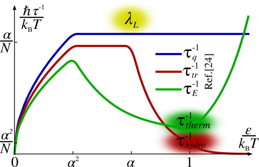
Figure 2: Qualitative representation of the energy dependence of the scattering rates, the dephasing rate $\tau_{q}^{-1}$, the rate relevant for transport processes $\tau_{tr}^{-1}$ and the energy relaxation rate $\tau_{E}^{-1}$, for weak coupling, $\alpha\ll 1$, obtained in Ref. Schuett2011 . Rates, which are relevant to hydrodynamic transport and energy relaxation, are determined by excitation energies $\epsilon\sim k_{B}T$ and are represented by a red or green spot. The determined scrambling rate $\lambda_{L}$ for weak coupling probing excitations predominantly at energies $\epsilon\sim\alpha k_{B}T$, is represented by a yellow spot. Scrambling processes at weak coupling are therefore a lot faster than the collisions that give rise to the hydrodynamic behavior of graphene, and also faster than the energy relaxation rate that one would expect to govern thermalization. Instead, the scrambling time in graphene is closely related to the dephasing scattering rate.

I The model

We consider the following Hamiltonian for electrons in graphene near the Dirac point with electron-electron Coulomb interaction (setting $\hbar=1$)

$$H =v\sum_{i=1}^{N}\int d^{2}\mathbf{x}\psi_{i}^{\dagger}\left(\mathbf{x}\right)\frac{1}{i}\mathbf{\nabla}\cdot\mathbf{\bm{\sigma}}\psi_{i}\left(\mathbf{x}\right)$$ (4)

$$+ \frac{e^{2}}{2}\sum_{\begin{subarray}{c}ij=1\\ \alpha\beta\end{subarray}}^{N}\int d^{2}\mathbf{x}d^{2}\mathbf{x}^{\prime}\frac{\psi_{i\alpha}^{\dagger}\left(\mathbf{x}\right)\psi_{j\beta}^{\dagger}\left(\mathbf{x}^{\prime}\right)\psi_{j\beta}\left(\mathbf{x}^{\prime}\right)\psi_{i\alpha}\left(\mathbf{x}\right)}{\left|\mathbf{x}-\mathbf{x}^{\prime}\right|}.$$

Here, $\psi_{i}=(\psi_{i1},\psi_{i2})^{\text{T}}$ is a two component spinor and $\mathbf{\bm{\sigma}}=(\sigma_{x},\sigma_{y})^{\text{T}}$ are Pauli matrices acting in pseudo-spin space. $i=1\dots N$ is an additional flavor index that includes spin and valley degrees of freedom. While $N=4$ for graphene, we keep $N$ arbitrary to be able to perform a controlled expansion in $1/N$ Son2007 ; Foster2008 . A key justification to use this approach for the description of graphene comes from experiment. Several measurements clearly reveal interactions effects Elias2011 ; Siegel2011 ; Yu2013 , but of a kind that is fully consistent with renormalization group assisted perturbation theory Sheehy2007 .

The retarded fermionic propagator, on the bare level given by

$$(G^{R})^{-1}=\left(\omega+i0^{+}\right)\sigma^{0}-v\mathbf{k}\cdot\bm{\sigma},$$ (5)

is dressed in leading order in $1/N$ by the usual rainbow diagram for the retarded self energy

$$\Sigma_{\alpha\beta}^{R}\left(\mathbf{k},\omega\right)=\frac{i}{2N}(D^{R}\circ G_{\alpha\beta}^{K}+D^{K}\circ G_{\alpha\beta}^{K})_{\left(\mathbf{k},\omega\right)},$$ (6)

where the superscripts $R$, $K$, and later $A$ stand for retarded, Keldysh, and advanced components of the Green’s functions, and $\circ$ stands for a convolution with regards to frequencies and momenta. $D^{-1}=D_{0}^{-1}+\Pi$ is the collective plasmon propagator with bare Coulomb interaction $D_{0}^{R}=\frac{2\pi e^{2}}{\left|\mathbf{q}\right|}$ and the bosonic self energy

$$\Pi^{R}\left(\mathbf{k},\omega\right)=\frac{i}{2}(G_{\alpha\beta}^{R}\circ G_{\beta\alpha}^{K}+G_{\alpha\beta}^{K}\circ G_{\beta\alpha}^{A})_{\left(\mathbf{k},\omega\right)}$$ (7)

which is of order $N^{0}$.

II Diagrammatic Approach

We start from the ’regularized’ version of the squared anticommutator

$$f_{\gamma\delta}^{\alpha\beta}\left(x_{1},x_{2},x_{3},x_{4}\right)=\frac{1}{N^{2}}\sum_{i,j=1}^{N}{\rm tr}\left(\left\{\psi_{i\alpha}\left(x_{1}\right),\psi_{j\beta}^{\dagger}\left(x_{2}\right)\right\}\right.\\ \times\left.\sqrt{\rho}\left\{\psi_{j\delta}\left(x_{4}\right),\psi_{i\gamma}^{\dagger}\left(x_{3}\right)\right\}\sqrt{\rho}\right)$$ (8)

where the regularization amounts to splitting the density matrix $\rho=Z^{-1}e^{-H/k_{B}T}$ between the two anticommutators Shenker2014 ; Maldacena2016 . Otherwise the exponent would depend explicitly on the UV cut-off of our effective field theory and would therefore be ill defined. $x=\left(\mathbf{x},t\right)$ stands for space and time coordinates. In order to determine the scrambling time, we analyze

$$C\left(t\right)=\theta\left(t\right)\int d^{2}\mathbf{x}\sum_{\alpha\beta}f_{\alpha\beta}^{\alpha\beta}\left(x,0,x,0\right),$$ (9)

which contains a correlator with non-trivial time order denoted out-of-time-order correlator (OTOC), i.e. sequences of operators which cannot be represented on a conventional Keldysh contour evolving back and forth in time.

II.1 Out-of-time-order formalism

To determine the function $f$, we use the out-of-time-order formalism and the corresponding four-branch (two-loop) Keldysh contour Aleiner2016 ; Stanford2016 . In this case, the thermal expectation value is expressed as expectation value of four-component Grassmann fields $\psi_{i\alpha}(t)=\left(\psi^{u+},\psi^{u-},\psi^{l+},\psi^{u-}\right)_{i\alpha,\left(t\right)}^{\text{T}}$, and analogously $\bar{\psi}_{i\alpha}$, placed on the Keldysh contour according to their relative causal position. The position of the fields is specified, besides the time parameter $t$, by the loop index $\sigma=\left\{u,l\right\}$ for the upper and lower loop, and the branch index $\left\{+,-\right\}$ denoting the branches propagating forward and backward in time, respectively. The contour including the position of the fractions of density matrices placed between the anticommutators is depicted in Fig. 3.

We perform the standard Keldysh rotation Kamenev2011 for each of the two loops $\sigma=\{u,l\}$ separately,

$$\psi^{\sigma\text{cl}} =\frac{1}{\sqrt{2}}\left(\psi^{\sigma+}+\psi^{\sigma-}\right),\,\psi^{\sigma\text{q}}=\frac{1}{\sqrt{2}}\left(\psi^{\sigma+}-\psi^{\sigma-}\right),$$

$$\bar{\psi}^{\sigma\text{cl}} =\frac{1}{\sqrt{2}}\left(\bar{\psi}^{\sigma+}-\bar{\psi}^{\sigma-}\right),\,\bar{\psi}^{\sigma\text{q}}=\frac{1}{\sqrt{2}}\left(\bar{\psi}^{\sigma+}+\bar{\psi}^{\sigma-}\right),$$ (10)

where Keldysh indices $s=\left\{\text{cl},\text{q}\right\}$ denote ’classical’- (cl) and ’quantum’- (q) field components, respectively.

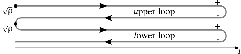
Figure 3: Two-loop Keldysh contour. Index $u$ and $l$ refer to the fields residing on the upper and lower Keldysh loop, index $+$ and $-$ to fields residing on the forward and backward propagating branch, respectively. The square roots of density matrices are placed at the left turning points of the contour denoted by solid black dots.

An effective Keldysh action is obtained by introducing real plasmon fields $\phi$ which couple linearly to a pair of fermion fields. For this, we carry out the standard Hubbard-Stratonovich transformation to decouple the interaction term of the Hamilton operator in Eq. 4 in the charge channel. Consequently, the quadratic part of the Keldysh action is given by (pseudo-spin and flavor indices are dropped):

$$S_{0}\left[\psi,\bar{\psi},\phi\right]=\sum_{\sigma^{(^{\prime})}s^{(^{\prime})}}\bigg{(}\int_{k}\bar{\psi}_{k}^{\sigma s}\,G_{\sigma\sigma^{\prime},ss^{\prime}}^{-1}(k)\,\psi_{k}^{\sigma^{\prime}s^{\prime}}+\\ +\int_{q}\phi_{-q}^{\sigma s}\,D_{\sigma\sigma^{\prime},ss^{\prime}}^{-1}(q)\,\phi_{q}^{\sigma^{\prime}s^{\prime}}\bigg{)},$$ (11)

where $k=\left(\epsilon,\mathbf{k}\right)$ and $\int_{k}=\int\frac{d\epsilon}{2\pi}\int\frac{d^{2}\mathbf{k}}{\left(2\pi\right)^{2}}$. The intra-loop components of the fermionic and bosonic plasmon propagators ($\sigma=\sigma^{\prime}$) have the usual causal structure

$$G_{\sigma\sigma,ss^{\prime}}=\begin{pmatrix}G^{R}&G^{K}\\ 0&G^{A}\end{pmatrix}_{ss^{\prime}}\text{, }D_{\sigma\sigma,ss^{\prime}}=\begin{pmatrix}D^{K}&D^{R}\\ D^{A}&0\end{pmatrix}_{ss^{\prime}}$$ (12)

where superscripts $R$/$A$ denote retarded and advanced components, and the fermionic and bosonic Keldysh components are given by $G^{K}\left(k\right)=2i\tanh(\frac{\epsilon}{2k_{B}T})\text{Im}G^{R}\left(k\right)$ and $D^{K}\left(k\right)=2i\coth(\frac{\epsilon}{2k_{B}T})\text{Im}D^{R}\left(k\right)$. In the case of inter-loop correlations ($\sigma^{\prime}=\bar{\sigma}$ where $\bar{u}=l$ and vice versa),

$$G_{\sigma\bar{\sigma},ss^{\prime}}=\begin{pmatrix}0&G_{\sigma\bar{\sigma}}^{K}\\ 0&0\end{pmatrix}_{ss^{\prime}}\text{, }D_{\sigma\bar{\sigma},ss^{\prime}}=\begin{pmatrix}D_{\sigma\bar{\sigma}}^{K}&0\\ 0&0\end{pmatrix}_{ss^{\prime}},$$ (13)

there is only a Keldysh components which relates to the retarded components as

$$D_{ul}^{K}(\omega,\mathbf{q}) =\frac{2i\text{Im}D^{R}(\omega,\mathbf{q})}{\sinh\left(\frac{\omega}{2k_{B}T}\right)},$$ (14a)

$$G_{lu,a}^{K}\left(\epsilon,\mathbf{k}\right) =\frac{2i\text{Im}G_{a}^{R}(\epsilon,\mathbf{k})}{\cosh\left(\frac{\epsilon}{2k_{B}T}\right)}=-G_{ul,a}^{K}\left(\epsilon,\mathbf{k}\right).$$ (14b)

Here, we use the band basis where the first term in Eq. 4 is diagonal and $G_{a}^{R}=\left(\omega+i0^{+}-av|\mathbf{k}|\right)^{-1}$ with $a=\pm 1$.

The fermionic and bosonic fields couple via the term

$$S_{\text{int}}\left[\psi,\bar{\psi},\phi\right]=\frac{1}{\sqrt{N}}\sum_{\sigma s^{(^{\prime},^{\prime\prime})}}\int_{kq}\bar{\psi}_{k+q}^{\sigma s}\psi_{k}^{\sigma s^{\prime}}\phi_{q}^{\sigma s^{\prime\prime}}\,\gamma_{ss^{\prime}}^{s^{\prime\prime}}.$$ (15)

which is weighted by a factor of $1/\sqrt{N}$. The coupling is diagonal in Keldysh-loops as well as all dropped indices. The coupling vertices acting in Keldysh component space are $\gamma_{ss^{\prime}}^{\text{cl}}=\delta_{ss^{\prime}}$ and $\gamma_{ss^{\prime}}^{\text{q}}=\left(\sigma_{1}\right)_{ss^{\prime}}$ with $\sigma_{1}$ being the first Pauli matrix.

Within this framework, the squared anticommutator Eq. 8 is recast as the expectation value of ’classical’- and ’quantum’-Keldysh field components

$$f_{\gamma\delta}^{\alpha\beta}\left(x_{1},x_{2},x_{3},x_{4}\right)=\\ -\frac{1}{N^{2}}\sum_{i,j=1}^{N}\langle\psi_{i\alpha}^{l\text{cl}}\left(x_{1}\right)\bar{\psi}_{j\beta}^{l\text{cl}}\left(x_{2}\right)\bar{\psi}_{i\gamma}^{u\text{q}}\left(x_{3}\right)\psi_{j\delta}^{u\text{q}}\left(x_{4}\right)\rangle_{\mathcal{K}}$$ (16)

which are evaluated with respect to the two-loop Keldysh action $\langle\dots\rangle_{\mathcal{K}}=\int\mathcal{D}\left(\bar{\psi},\psi,\phi\right)\dots e^{i\mathcal{S}_{\mathcal{K}}\left[\psi,\phi\right]}$ with $S_{\mathcal{K}}=S_{0}+S_{\text{int}}$. Eventually, contributions of $S_{\text{int }}$ to $f$ are incorporated perturbatively in orders of $1/N$.

II.2 Bethe-Salpeter equation

(a)

(b)

(c)

(d)

Figure 4: Diagrammatic representation of processes contributing to scrambling in leading order in $1/N$. Straight lines correspond to bare fermion propagators, wavy lines to plasmon propagators dressed by particle-hole fluctuations. Both types of propagators are of order $N^{0}$. Each interaction vertex contributes a factor of $1/\sqrt{N}$, whereas each fermion loop a factor of $N$. Propagators residing on the upper or lower horizontal line are located on one of the Keldysh loops, vertical propagators are loop-connecting propagators causing scrambling. (a) One-rung diagram containing one inter-loop bosonic propagator. (b) Two-rung diagram containing two inter-loop fermionic propagators. An extra factor of $N$ is obtained by an additional closed fermion loop and is therefore of order $\mathcal{O}(1/N)$. The crossed-rung diagram in (c) vanishes exactly as the retarded and advanced inter-loop components (see Eq. 13) are zero. (d) Diagrammatic representation of self-consistent Bethe-Salpeter equation for $f(\omega,k)$ in leading order in $1/N$.

Interaction processes contributing to scrambling involve inter-loop correlators. The leading order processes in $1/N$ are depicted in Fig. 4a and 4b as diagrammatic representation. To capture the exponential growth behavior of Eq. 9, these diagrams are summed in an infinite ladder series. Note that irreducible contributions which are of higher order in $1/N$ yield corrections to the growth rate $\lambda_{L}$ of higher order and are therefore neglected. The diagrammatic series is derived by considering the Laplace transform of Eq. 8 where half of the internal degrees of freedom are already traced out:

$$\begin{split}f_{\beta}^{\alpha}(\omega,k)&\equiv\int_{\epsilon^{\prime}\mathbf{k^{\prime}}}\int_{x_{1}x_{2}x_{3}}\sum_{\gamma}f_{\beta\gamma}^{\alpha\gamma}(x_{1},x_{2},x_{3},0)\\ \times&e^{i\left(\omega+\epsilon^{\prime}\right)t_{1}-i\left(\omega+\epsilon\right)t_{2}-i\epsilon t_{3}-i\mathbf{k}\cdot\left(\mathbf{x}_{1}-\mathbf{x}_{3}\right)+i\mathbf{k}^{\prime}\cdot\mathbf{x}_{2}}\\ &\equiv\,\,\vbox{\hbox{\includegraphics[height=42.00003pt]{InlineDiagram.pdf}}}\end{split}$$ (17)

with $k=\left(\epsilon,\mathbf{k}\right)$, $\int_{k}=\int\frac{d\epsilon}{2\pi}\int\frac{d^{2}\mathbf{k}}{\left(2\pi\right)^{2}}$ and $\int_{x}=\int dt\int d^{2}\mathbf{x}$. The resulting Bethe-Salpeter equation, which determines $f$ recursively, is given by

$$f_{\beta}^{\alpha}\left(\omega,k\right)=\frac{1}{N}\sum_{\gamma}G_{\alpha\gamma}^{R}(\omega+\epsilon,\mathbf{k})G_{\gamma\beta}^{A}(k)+\qquad\qquad\quad$$ (18)

$$\frac{1}{N}\int_{k^{\prime}}\sum_{\gamma^{(^{\prime})}\delta^{(^{\prime})}}f_{\delta^{\prime}}^{\gamma^{\prime}}(\omega,k^{\prime})\Gamma_{\delta\delta^{\prime}}^{\gamma\gamma^{\prime}}\left(\omega,k,k^{\prime}\right)G_{\alpha\gamma}^{R}(\omega+\epsilon,\mathbf{k})G_{\delta\beta}^{A}(k)$$

and depicted in Fig. 4d as diagrammatic representation. The inter-loop scattering vertex $\Gamma$ contains one-rung (first term) and two-rung (second term) contributions,

$$\Gamma_{\gamma\delta}^{\alpha\beta}\left(\omega,k,k^{\prime}\right)=i\delta_{\alpha\beta}\delta_{\gamma\delta}D_{ul}^{K}(k-k^{\prime})\\ +\int_{\tilde{k}}G_{\alpha\gamma}^{lu}(k-\tilde{k})G_{\delta\beta}^{ul}(k^{\prime}-\tilde{k})D^{R}(\omega+\tilde{\epsilon},\tilde{\mathbf{k}})D^{A}(\tilde{k}),$$ (19)

shown in Fig. 4(a) and (b), respectively.

Focusing on the leading contribution to $\lambda_{L}$ in our large-$N$ expansion allows to perform a series of simplifications of Eq. 18. First, we set the fermionic propagators on mass-shell which requires a representation in diagonal band-basis and which implicitly assumes that a quasi-particles description is applicable. We therefore introduce the projection operator ${\mathcal{P}}_{\alpha\beta}^{a}\left(\mathbf{k}\right)$ for the two bands $a=\pm 1$ which connects the pseudo-spin- and band-basis by $G_{\alpha\beta}^{R}\left(k\right)=\sum_{a}\mathcal{P}_{\alpha\beta}^{a}\left(\mathbf{k}\right)G_{a}^{R}\left(k\right)$. The projection operator has the properties $\sum_{\alpha}\mathcal{P}^{a}_{\alpha\alpha}\left(\mathbf{k}\right)=1$ and $\sum_{\beta}\mathcal{P}_{\alpha\beta}^{a}\left(\mathbf{k}\right)\mathcal{P}_{\beta\gamma}^{b}\left(\mathbf{k}^{\prime}\right)=\frac{1}{2}\mathcal{P}_{\alpha\gamma}^{a}\left(\mathbf{k}\right)(1+ab\frac{\mathbf{k}\cdot\mathbf{k}^{\prime}}{|\mathbf{k}||\mathbf{k}^{\prime}|})$, for $a,b=\pm 1$. This allows us to replace the product of Green’s functions by

$$G_{\alpha\gamma}^{R}(\omega+\epsilon,\mathbf{k})G_{\delta\beta}^{A}\left(\epsilon,\mathbf{k}\right)\\ =2\pi i\frac{\mathcal{P}_{\alpha\gamma}^{a}(\mathbf{k})\mathcal{P}_{\delta\beta}^{b}(\mathbf{k})\delta\left(\epsilon-av|\mathbf{k}|\right)}{\omega-\left(a-b\right)|\mathbf{k}|+i0^{+}}.$$ (20)

To focus on the most rapidly growing term, we restrict Eq. 20 to $a=b$ and set the frequency of the scattering vertex in Eq. 19 to zero, $\Gamma_{\gamma\delta}^{\alpha\beta}(\omega,k,k^{\prime})|_{\omega=0}$.

Furthermore, to leading order in $1/N$, the squared anticommutator is expressed by one band index only

$$f_{\beta}^{\alpha}\left(\omega,k\right)=\sum_{a=\pm 1}f_{a}\left(\omega,\mathbf{k}\right)\mathcal{P}_{\alpha\beta}^{a}\left(\mathbf{k}\right)2\pi\delta(\epsilon-av|\mathbf{k}|).$$ (21)

Exploiting particle-hole symmetry, determining the Lyapunov exponent is eventually reduced to solving the integral equation

$$f(\omega,\mathbf{k})=\frac{i}{\omega}\frac{1}{N}\Big{(}1+\int_{\mathbf{k}^{\prime}}M(\mathbf{k},\mathbf{k}^{\prime})\,f(\omega,\mathbf{k}^{\prime})\Big{)}$$ (22)

where $f(\omega,\mathbf{k})=\int_{\epsilon}\sum_{\alpha}f_{\alpha}^{\alpha}(\omega,k)$ with the kernel $M=M_{+}+M_{-}$ comprised out of band-preserving ($+$) and band-changing ($-$) processes

$$M_{\text{$\pm$}}(\mathbf{k},\mathbf{k}^{\prime})=i\,K_{\pm+}\left(\mathbf{k},\mathbf{k}^{\prime}\right)D_{ul}^{K}(|\mathbf{k}^{\prime}|\mp|\mathbf{k}|,\mathbf{k}^{\prime}\mp\mathbf{k})\\ +\sum_{a^{\prime}b^{\prime}}\int_{\tilde{k}}K_{+b^{\prime}}(\mathbf{k}^{\prime},\mathbf{k}^{\prime}-\tilde{\mathbf{k}})\,K_{\pm a^{\prime}}(\mathbf{k},\mathbf{k}-\tilde{\mathbf{k}})\\ \times G_{a^{\prime}}^{ul}(\text{$\pm$}a^{\prime}|\mathbf{k}|-\tilde{\epsilon},\mathbf{k}-\tilde{\mathbf{k}})G_{b^{\prime}}^{lu}(b^{\prime}|\mathbf{k}^{\prime}|-\tilde{\epsilon},\mathbf{k}^{\prime}-\tilde{\mathbf{k}})\\ \times D^{R}(\tilde{\epsilon},\tilde{\mathbf{k}})D^{A}(\tilde{\epsilon},\tilde{\mathbf{k}})$$ (23)

where $K_{ab}\left(\mathbf{k},\mathbf{k}^{\prime}\right)\equiv\frac{1}{2}(1+ab\frac{\mathbf{k}\cdot\mathbf{k}^{\prime}}{|\mathbf{k}||\mathbf{k}^{\prime}|})$. The first term represents one-rung (denoted by $M_{\pm}^{(1)}$ in the following) and the second term two-rung scattering, see Fig. 4d.

The Lypanuov exponent is finally determined by finding the set of eigenvalues $\{\lambda\}$ and corresponding eigenfunctions $\{f^{\prime}\}$ of $M(\textbf{k},\textbf{k}^{\prime})$. Being real and symmetric, it is possible to bring the kernel in diagonal form,

$$M^{\prime}(\textbf{k},\textbf{k}^{\prime})=\\ \int_{\textbf{q}\textbf{q}^{\prime}}V(\textbf{k},\textbf{q})M(\textbf{q},\textbf{q}^{\prime})V(\textbf{q}^{\prime},\textbf{k}^{\prime})=N\lambda_{\textbf{k}}\delta(\textbf{k}-\textbf{k}^{\prime})$$ (24)

where the linear orthonormal transformation is described by the orthogonal matrix $V$. Using Eq. 22, we get

$$f^{\prime}(\textbf{k},\omega)=\frac{i}{\omega}\frac{1}{N}\left[e_{\textbf{k}}+N\lambda_{\textbf{k}}f^{\prime}(\textbf{k},\omega)\right]$$ (25)

where $f^{\prime}(\textbf{k},\omega)=\int_{\textbf{q}}V(\textbf{k},\textbf{q})f(\textbf{q},\omega)$ and $e_{\textbf{k}}=\int_{\textbf{q}}V(\textbf{k},\textbf{q})$. Applying the inverse Fourier transform $\int\frac{d\omega}{2\pi}\frac{e^{-i\omega t}}{(\omega+i0^{+})^{n+1}}=(-i)^{n+1}\theta(t)\frac{t^{n}}{n!}$, we find

$$f^{\prime}(\textbf{k},t)=\frac{e_{\textbf{k}}}{N}\sum_{n=0}^{\infty}\frac{(\lambda_{\textbf{k}}t)^{n}}{n!}=\frac{e_{\textbf{k}}}{N}e^{\lambda_{\textbf{k}}t}$$ (26)

which represents the desired exponential growth behavior described by the spectrum of growth exponents $\lambda_{\textbf{k}}$ (see also Appendix D).

The Lyapunov exponent is now defined as $\lambda_{L}=\max[\lambda_{\textbf{k}}]$, and the corresponding eigenfunction is denoted $f^{\prime}_{L}$. Consequently, the Lyapunov exponent can be efficiently determined as the largest eigenvalue of the eigenvalue equation

$$\lambda\,f(\textbf{k},\omega)=\int_{\textbf{k}^{\prime}}M(\mathbf{k},\mathbf{k}^{\prime})f(\mathbf{k}^{\prime},\omega)$$ (27)

instead of solving the inhomogeneous Eq. 22. An explicit representation of the homogeneous Bethe-Salpeter equation, which is solved numerically, can be found in App. B.

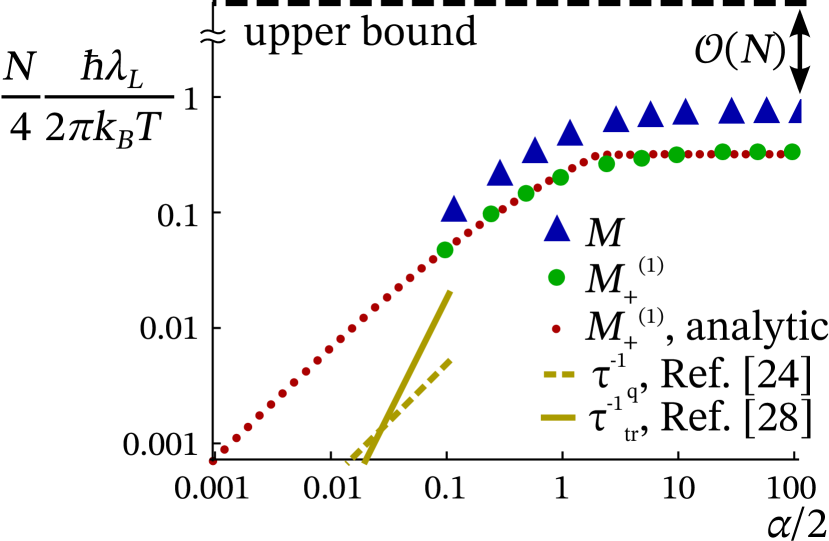
Figure 5: The Lyapunov exponent as a function of coupling $\alpha$ to leading order in $1/N$: Blue triangles and green dots represent values obtained using the full kernel $M$ and focusing on the one-rung contribution $M_{+}^{(1)}$, respectively. We use a grid of $2^{9}\times 2^{9}$ points in momentum space. These results are compared to values (red dots) obtained by an analytic approximation for $M_{+}^{(1)}$ of Eq. 28 which is solved iteratively with much higher precision. A linear function is fitted to the data points for $\alpha\ll 1$. We find that $\lambda_{L}=C\,\alpha\frac{4}{N}\frac{2\pi k_{B}T}{\hbar}$ with $C=0.37$ (see Appendix C for more details on the numerical procedure). The solid and dashed yellowish lines represent the dephasing rate $\tau_{q}^{-1}$ evaluated at $\epsilon\approx\alpha k_{B}T$ and the transport rate $\tau_{\text{tr}}^{-1}$ obtained from Ref. Schuett2011 and Ref. Fritz2008 , respectively.

II.3 Results

The Lyapunov exponent as a function of coupling $\alpha$ is depicted in Fig. 5. It saturates for strong coupling to the asymptotic value given in Eq. 2. Even if we extrapolate the number of fermion flavors to its physical value $N=4$ the mentioned bound is not saturated. For weak coupling, we obtain Eq. 3.

For our subsequent discussion it is important to determine the corresponding eigenfunctions of the kernel $M(\mathbf{k},\mathbf{k}^{\prime})$. We find that in the case of strong coupling the eigenfunction $f_{L}\left(|\mathbf{k}|\right)$ is peaked at energies of order of the temperature, $v|\mathbf{k}|\approx k_{B}T$, which is the only energy scale present, see Fig. 6. In the weak coupling regime however, the peak shifts due to the finiteness of the coupling to $v|\mathbf{k}|\propto\alpha k_{B}T$ which is the scale associated with the thermal screening of the Coulomb interaction Schuett2011 .

As shown in Fig. 5, the dominant contribution to scrambling in graphene is the one-rung band-preserving scrambling process $M_{+}^{(1)}$. The Bethe-Salpeter equation only taking into account $M_{+}^{(\text{1})}$ is given by

$$\lambda f(\omega,K) =\frac{2\pi k_{B}T}{\hbar}\frac{4}{N}\,\frac{2}{K}\int_{0}^{\infty}\frac{dK^{\prime}}{2\pi}\int_{|K-K^{\prime}|}^{|K+K^{\prime}|}\frac{QdQ}{2\pi}$$ (28)

$$\times \frac{\sqrt{\left(K+K^{\prime}\right)^{2}-Q^{2}}}{\sqrt{Q^{2}-\left(K-K^{\prime}\right)^{2}}}\frac{\text{Im}\mathcal{D}^{R}\left(|K-K^{\prime}|,Q\right)}{\sinh\left(|K-K^{\prime}|\right)}\,f(\omega,K^{\prime})$$

where we introduced the dimensionless momenta $K=\frac{v|\mathbf{k}|}{2k_{B}T}$ and the dimensionless imaginary part of the propagator $\text{Im}\mathcal{D}^{R}$ (see Appendix B for its definition). In the co-scattering limit $K\sim K^{\prime}$, and transferred momenta smaller than the thermal screening scale $Q\leq L_{\text{s }}^{-1}\ll 1$ where $L_{\text{s }}^{-1}=l_{s}^{-1}\hbar v/k_{B}T=\alpha\,\ln 2$, the kernel (up to phase space factors) is

$$\frac{2Q\,\text{Im}\mathcal{D}_{ul}^{R}\left(|K-K^{\prime}|,Q\right)}{\sinh\left(|K-K^{\prime}|\right)}\overset{K\rightarrow K^{\prime}}{=}\frac{\alpha^{2}\ln 2\,}{\left(Q+\alpha\ln 2\right)^{2}}$$ (29)

which approaches $1/\ln 2$ for $Q\ll\alpha$. We note that the dressed interaction becomes independent of coupling due to thermal screening processes Schuett2011 . Thus, the dominating scrambling takes place on orders of the screening scale $L_{\text{s}}^{-1}$ induced by finite coupling. This is reflected in the overall result for the Lyapunov exponent: The exponent is linear in coupling due to interactions of order $\alpha^{0}$ which holds for transferred energies smaller than the screening scale $L_{\text{s}}^{-1}\propto\alpha$.

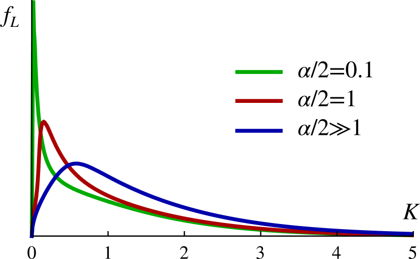
Figure 6: Eigenfunctions corresponding to the largest eigenvalue $\lambda_{L}$ as a function of energy for three different couplings. In the plot, $K=\frac{v|\mathbf{k}|}{2k_{B}T}$. In the case of strong coupling, the eigenfunction is peaked at energies $v|\mathbf{k}|\approx k_{B}T$ which is the only energy scale present. For weak coupling, the peak shifts to $v|\mathbf{k}|\propto\alpha k_{B}T$ which relates to an energy scale induced by finite coupling.

In order to interpret our result, Eq. 3 for weak coupling, we compare $\lambda_{L}$ with the characteristic energy scales discussed in Schuett2011 . This discussion is most transparent if we focus on Eq. 28. The kernel behaves qualitatively as the one for the relaxation rate $\tau_{q}^{-1}\left(\epsilon\right)$ of Schuett2011 , i.e. there are no $1-\cos^{2}\theta_{\mathbf{k},\mathbf{k}^{\prime}}$ back-scattering corrections that enter the transport rate $\tau_{\text{tr}}^{-1}\left(\epsilon\right)$ or energy weights $\propto(K-K^{\prime})^{2}$ that determine the energy relaxation rate $\tau_{E}^{-1}\left(\epsilon\right)$, respectively. For details see also Fig. 2 and the Appendix A. Furthermore, our eigenfunctions vary on a scale $\alpha k_{B}T$, see Fig. 6. Projection to energy scales $\alpha k_{B}T$ amounts essentially to setting the typical energy scale $\epsilon\approx\alpha k_{B}T$. In this limit follows indeed from Ref. Schuett2011 that $\tau_{q}^{-1}(\epsilon=\alpha k_{B}T)\approx 0.58\alpha k_{B}T/\hbar N$ similar to our scrambling rate. While there are differences in the detailed numerical prefactors – the coefficient of $\lambda_{L}$ is about 16 times larger, see Fig. 5 – the scrambling rate in graphene behaves as a dephasing rate. For weak coupling this scale is much faster than the characteristic transport collision rate of the hydrodynamic regime $\tau_{{\rm tr}}^{-1}\sim\alpha^{2}k_{B}T/\hbar N$, guaranteeing local thermalization which is a key prerequisite of a hydrodynamic description. Since $\lambda_{L}\gg\tau_{E}^{-1}$ for energies between $\alpha k_{B}T$ and $k_{B}T$ we also find that actual thermalization is a much slower processes than information scrambling.

III Kinetic equation

In this section we present an alternative approach to describe the spread of information in time and space in many-body systems. In contrast to the diagrammatic expansion conducted in the previous section, we show that scrambling is described by an integro-differential equation similar to the well-known Boltzmann equation. It describes the growth of an initially small, localized perturbation.

The process of information scrambling is governed by two scales: The Lyapunov exponent $\lambda_{L}$ and the Butterfly velocity $v_{B}=\sqrt{4D\lambda_{L}}$ which gives rise to an additional length scale $l_{B}=\frac{v_{B}}{\lambda_{L}}$ associated with the spatial spreading of information. For the system discussed in this work, the scrambling parameters are small $\lambda_{L},l_{B}^{-1}\sim\mathcal{O}\left(1/N\right)$. Based on the smallness of these parameters we propose that the spreading of information and the exponential growth signaling chaotic behavior is described by a quantity $f(t,\mathbf{x})$ which is governed by the partial differential equation

$$\partial_{t}f-D\Delta_{\mathbf{x}}f=f_{0}\delta\left(t\right)\delta\left(\mathbf{x}\right)+\lambda_{L}f,$$ (30)

where higher order gradient terms are suppressed in higher orders of $\lambda_{L}$ and $l_{B}^{-1}$. The LHS represents a diffusion equation characterized by diffusion constant $D$, whereas the RHS contains a source term and a term $\sim\lambda_{L}$ that indicates that $f$ is not a conserved quantity: A perturbing term $f_{0}\ll 1$ triggering the onset of growth and a second term causing the characteristic exponential growth behavior. Eq. 30 is valid for early times, i.e. $0<t-\frac{|\mathbf{x}|}{v_{B}}<t^{*}$ with the scrambling time $t^{*}\sim\lambda^{-1}\log N$. For times $t-\frac{|\mathbf{x}|}{v_{B}}>t^{*},$ non-linear terms are relevant causing $f$ to saturate against its asymptotic long-time value.

The solution of Eq. 30 is obtained by Fourier transform and is given by

$$f(\mathbf{x},t)=\frac{f_{0}}{4\pi Dt}e^{\lambda_{L}t-\frac{\mathbf{x}^{2}}{4Dt}}\approx\frac{f_{0}}{4\pi Dt}e^{2\lambda_{L}\left(t-\frac{|\mathbf{x}|}{v_{B}}\right)}$$ (31)

where the approximative result is obtained for $|\mathbf{x}|\approx v_{B}t$. It suggests that information spreads diffusively. However, due to the additional source term in Eq. 30 spreading is enhanced and the perturbation propagates ’quasi-ballistically’ as indicated by the approximative solution Eq. 31.

In the following section we derive Eq. 30 microscopically for the specific case of graphene. The approach is however more general and also applicable to other systems which can be treated perturbatively.

III.1 Derivation

We start by introducing a generating field $W$ which allows us to express the correlation function containing OTOCs introduced in Eq. 8 as functional derivative. It is introduced by directly coupling to the inter-loop fermionic density

$$S^{\prime}[W]=-\frac{1}{N}\int_{x}\sum_{i\alpha}W_{i\alpha}(x_{1},x_{2})\bar{\psi}_{i\alpha}^{l\text{cl}}(x_{1})\psi_{i\alpha}^{u\text{q}}(x_{2})$$ (32)

which enters as a contribution to the effective two-loop Keldysh action $S^{\prime}_{\mathcal{K}}=S_{\mathcal{K}}+S^{\prime}$. Consequently, the correlation function is obtained as a functional derivative of the fermionic inter-loop Keldysh component $G_{lu,\alpha\beta}^{K}(x_{1},x_{2};W)=-i\langle\psi_{i\alpha}^{l\text{cl}}(x_{1})\bar{\psi}_{i\beta}^{u\text{q}}(x_{2})\rangle$:

$$f_{\beta\gamma}^{\alpha\gamma}(x_{1},x_{2},x_{3},0)=-\frac{1}{N}\frac{\delta G_{lu,\alpha\beta}^{K}(x_{1},x_{3};W)}{\delta W_{j\gamma}(x_{2},0)}\bigg{|}_{W=0}$$ (33)

We are therefore interested in the dependence of $G_{lu}^{K}$ on the field $W$, which can be interpreted as the evolution of $G_{lu}^{K}$ in time and spatial space due to an earlier localized perturbation.

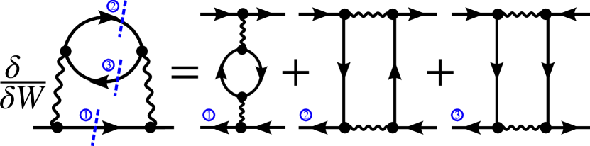
Figure 7: Leading order self-energy diagram in the large-$N$, weak-coupling ($\alpha\ll 1$) regime. Dashed blue lines represent functional derivatives applied to obtain the linearized kinetic equations in Eq. 42.

The dynamics of the Keldysh components are conveniently described by means of kinetic equations, an established approach to non-equilibrium problems (see e.g. Ref. Kamenev2011 ). We therefore introduce the usual parametrization of $G^{K}$ applied to the inter-loop Keldysh components as

$$G_{lu,a}^{K} = G_{a}^{R}\circ H_{a}^{lu}-H_{a}^{lu}\circ G_{a}^{A},$$ (34a)

$$G_{ul,a}^{K} = G_{a}^{R}\circ H_{a}^{ul}-H_{a}^{ul}\circ G_{a}^{A},$$ (34b)

where conceptually non-equilibrium aspects are stored in the inter-loop distribution functions $H_{a}^{lu}\left(x_{1},x_{2}\right)$ and $H_{a}^{ul}\left(x_{1},x_{2}\right)$, $a$ represents the band-index and $\circ$ stands for a convolution with regards to time and spatial space. In equilibrium, $H^{lu,\left(\text{eq}\right)}\left(\epsilon,\mathbf{k}\right)=\cosh^{-1}(\frac{\epsilon}{2k_{B}T})=-H^{ul,\left(\text{eq}\right)}\left(\epsilon,\mathbf{k}\right)$, as already indicated in Eq. 14b. Within the concept of single particle self-energies, equations of motions of inter-loop distributions functions are obtained by using Dyson’s equation for intra- and inter-loop single-particle propagator components and are given in the presence of the generating field by

$$-\left[G_{a}^{-1}\overset{\circ}{,}H_{a}^{lu}\right] =$$

$$\frac{W}{N}+ \Sigma_{lu,a}^{K}-\left(\Sigma_{a}^{R}\circ H_{a}^{lu}-H_{a}^{lu}\circ\Sigma_{a}^{A}\right),$$ (35a)

$$-\left[G_{a}^{-1}\overset{\circ}{,}H_{a}^{ul}\right] =\Sigma_{ul,a}^{K}-\left(\Sigma_{a}^{R}\circ H_{a}^{ul}-H_{a}^{ul}\circ\Sigma_{a}^{A}\right).$$ (35b)

The expression for the inter-loop Keldysh self-energy is given by $\Sigma_{lu}^{K}=\frac{i}{2N}G_{lu}^{K}\left(x_{1},x_{2}\right)D_{ul}^{K}\left(x_{1},x_{2}\right)$, whereas the retarded and advanced components are as indicated in Sec. I. For convenience, we replace the bosonic Keldysh components by $D_{ul}^{K}=-D^{R}\circ\Pi_{ul}^{K}\circ D^{A}$ with the inter-loop Keldysh polarization operator $\Pi_{ul}^{K}\left(x_{1},x_{2}\right)=\frac{i}{2}G_{ul}^{K}\left(x_{1},x_{2}\right)G_{lu}^{K}\left(x_{2},x_{1}\right)$ to eliminate the bosonic Keldysh components. This expansion holds in the large-$N$, weak coupling limit, which shows the interesting behavior as discussed in the previous section. A diagrammatic representation of the considered self-energy contribution is depicted in Fig. 7.

In the derivation of the equations of motions Eq. 35 it was furthermore implicitly assumed that in the presence of interactions the band index remains a ’good’ quantum number, i.e. the unitary transformation represented by the matrix $\left(\mathcal{U}_{\alpha a,\textbf{k}}\right)$, which diagonalizes the free single-particle $\sum_{a}\mathcal{U}_{\alpha a,\mathbf{k}}^{\dagger}G_{a}(k)\mathcal{U}_{a\beta,\mathbf{k}}=G_{\alpha\beta}(k)$ model, diagonalizes also the self-energy expressions $\sum_{a}\mathcal{U}_{\alpha a,\mathbf{k}}^{\dagger}\Sigma_{a}(k)\mathcal{U}_{a\beta,\mathbf{k}}=\Sigma_{\alpha\beta}(k)$. This assumption proves legitimate in the low-temperature limit Schuett2011 .

As a next step, we introduce center-of-mass coordinates $X=\frac{1}{2}(x_{1}+x_{2})$ and derivations thereof $x=x_{1}-x_{2}$, respectively, and replace all quantities by quantities depending on these coordinates $Q(x_{1},x_{2})\rightarrow\tilde{Q}\left(X,x\right)$. The Wigner-transform is subsequently introduced as $\tilde{Q}(X,p)=\int_{x}e^{i(\omega t-\textbf{p}\cdot\textbf{x})}\tilde{Q}(X,x)$. Gradient terms, which are generated by Wigner-transforming convolution terms, are assumed to be small as argued in the introductory part of this section resulting in

$$-iZ^{-1}\left(\partial_{T}+\mathbf{v}_{\mathbf{p}}^{*}\cdot\nabla_{\mathbf{X}}\right)\tilde{H}_{a}^{lu} =$$

$$\frac{\tilde{W}}{N}+\tilde{\Sigma}_{lu,a}^{K}-\tilde{H}_{a}^{lu}\big{(}\tilde{\Sigma}_{a}^{R} -\tilde{\Sigma}_{a}^{A}\big{)}+F[\Delta\tilde{H}],$$ (36a)

$$-iZ^{-1}\left(\partial_{T}+\mathbf{v}_{\mathbf{p}}^{*}\cdot\nabla_{\mathbf{X}}\right)\tilde{H}_{a}^{ul} =$$

$$\tilde{\Sigma}_{ul,a}^{K}-\tilde{H}_{a}^{ul}\big{(}\tilde{\Sigma}_{a}^{R} -\tilde{\Sigma}_{a}^{A}\big{)}+F[\Delta\tilde{H}],$$ (36b)

where $\tilde{H}_{a}(T,\mathbf{X},\epsilon,\mathbf{p})$ denote the Wigner-transformed distribution functions which are assumed, besides the external generating field $\tilde{W}$, to be the only quantities depending on center-of-mass coordinates. First order gradient terms renormalize the single-particle parameters, such as the quasi-particle weight $Z=(1-\partial_{\epsilon}\text{Re}\tilde{\Sigma}_{a}^{R})^{-1}$ ($Z\approx 1$ in the case of graphene Schuett2011 ) and the renormalized group velocity $\mathbf{v}_{\mathbf{p}}^{*}=v_{F}Z\nabla_{\mathbf{p}}(\epsilon_{\mathbf{p}}+\text{Re}\tilde{\Sigma}_{a}^{R})$, whereas terms of second order gradients are stored in the term $F[\Delta_{\mathbf{x}}\tilde{H}]$. These second order gradient terms eventually give rise to spatial gradient terms as postulated in Eq. 30, which are however dropped in the ongoing discussion as their explicit form does not yield any new insights.

The single-particle spectral function $A_{a}\left(\epsilon,\mathbf{p}\right)=-\text{Im}\tilde{G}_{a}^{R}\left(\epsilon,\mathbf{p}\right)$ is peaked for $\epsilon\approx\epsilon_{\mathbf{p}}$. If the momentum dependence of $\text{Im}\Sigma_{a}^{R}$ is negligible, which is the case for graphene Schuett2011 , the spectrum contains no incoherent background and the quasi-particle description applies Woelfle2018 . This allows us to integrate out the frequency dependence to define the quasi-particle distribution function

$$h_{a\textbf{p}}(T,\mathbf{X}) = \int_{\epsilon}2A_{a}\left(\epsilon,\mathbf{p}\right)\tilde{H}_{a}\left(T,\mathbf{X},\epsilon,\mathbf{p}\right).$$ (37)

In the following we, approximate $A_{a}\left(\epsilon,\mathbf{p}\right)\approx\pi\delta\left(\epsilon-\epsilon_{\mathbf{p}}\right)$ and conduct the frequency integration which is identical to the mass-shell approximation conducted in the previous section withing the diagrammatic approach, see Eq. 20 and 21.

We eventually arrive at the following set of coupled partial differential equations

$$(\partial_{T}\negthinspace+\negthinspace\mathbf{v}_{\mathbf{p}}^{*}\cdot\nabla_{\mathbf{X}})h_{a\mathbf{p}}^{lu}\left(T,\mathbf{X}\right)\negthinspace-\negthinspace\frac{W_{a\mathbf{p}}}{N} =I\left[h^{lu},h^{ul}\right],$$ (38a)

$$\left(\partial_{T}+\mathbf{v}_{\mathbf{p}}^{*}\cdot\nabla_{\mathbf{X}}\right)h_{a\mathbf{p}}^{ul}\left(T,\mathbf{X}\right) =I\left[h^{ul},h^{lu}\right],$$ (38b)

where the mass-shell restricted generating field reads $W_{a\mathbf{p}}\left(T,\mathbf{X}\right)=i\int_{\epsilon}2A_{a}\left(\epsilon,\mathbf{p}\right)W\left(T,\mathbf{X},\epsilon,\mathbf{p}\right)$. In analogy to the quasi-classical Boltzmann equation, we introduced a ’collision-integral’ $I[h^{lu},h^{ul}]$ (and conversely $I[h^{ul},h^{lu}]$ which is obtained by exchanging $h^{ul}\leftrightarrow h^{lu}$) on the RHSs of the previous equation which represents interaction processes coupling the different components of $h^{ul}$ and $h^{lu}$. It is given by

$$I\left[h^{lu},h^{ul}\right]=\\ \negthinspace-\frac{\pi}{2N}\negthinspace\negthinspace\sum_{a^{\prime}bb^{\prime}}\int_{\mathbf{qk}}\negthinspace\negthinspace\negthinspace\negthinspace\delta(\epsilon_{a\mathbf{p}}\negthinspace-\negthinspace\epsilon_{b\mathbf{k}}\negthinspace+\negthinspace\epsilon_{b^{\prime}\mathbf{q+k}}\negthinspace-\negthinspace\epsilon_{a^{\prime}\mathbf{p+q}})\negthinspace\negthinspace\times\negthinspace\negthinspace|T_{a^{\prime}bab^{\prime}}(\mathbf{p},\mathbf{k},\mathbf{q})|^{2}\\ \negthinspace\times\negthinspace\bigg{[}h_{a^{\prime}\mathbf{p+q}}^{lu}h_{b^{\prime}\mathbf{q+k}}^{ul}h_{b\mathbf{k}}^{lu}\negthinspace-\negthinspace\frac{h_{a^{\prime}\mathbf{p+q}}^{lu,(\text{eq})}h_{b^{\prime}\mathbf{q+k}}^{ul,(\text{eq})}h_{b\mathbf{k}}^{lu,(\text{eq})}}{h_{a\mathbf{p}}^{lu,(\text{eq})}}h_{a\mathbf{p}}^{lu}\bigg{]}$$ (39)

where the $\delta$-function ensures energy conservation, the interaction matrix-element $T$, which is given by $T_{a^{\prime}bab^{\prime}}(\mathbf{p},\mathbf{k},\mathbf{q})=\tilde{D}_{\mathbf{q}}(U_{\mathbf{p}}U_{\mathbf{p}+\mathbf{q}}^{\dagger})_{aa^{\prime}}(U_{\mathbf{q}+\mathbf{k}}U_{\mathbf{k}}^{\dagger})_{b^{\prime}b}$ in the case of graphene, and the equilibrium distribution functions $h_{a\mathbf{p}}^{lu,(\text{eq})}=\cosh^{-1}(\frac{\epsilon_{a\mathbf{p}}}{2k_{B}T})=-h_{a\mathbf{p}}^{ul,(\text{eq})}$. To derive the second term the intra-loop distribution functions were replaced by their equilibrium value as being not affected by $W_{a\textbf{p}}$ and it was used that

$$h^{(\text{eq})}_{b^{\prime}\mathbf{q+k}}h^{(\text{eq})}_{b\mathbf{k}}-h^{(\text{eq})}_{a^{\prime}\mathbf{p+q}}h^{(\text{eq})}_{b\mathbf{k}}+h^{(\text{eq})}_{a^{\prime}\mathbf{p+q}}h^{(\text{eq})}_{b^{\prime}\mathbf{q+k}}-1\\ =\frac{h_{a^{\prime}\mathbf{p+q}}^{lu,(\text{eq})}h_{b^{\prime}\mathbf{q+k}}^{ul,(\text{eq})}h_{b\mathbf{k}}^{lu,(\text{eq})}}{h_{a\mathbf{p}}^{lu,(\text{eq})}}$$ (40)

with the equilibrium intra-loop distribution function $h^{(\text{eq})}_{a\mathbf{k}}=\tanh(\frac{\epsilon_{a\mathbf{k}}}{2k_{B}T})$. In equilibrium, the collision-integral vanishes, i.e. $I[h_{a\mathbf{p}}^{lu,(\text{eq})},h_{a\mathbf{p}}^{ul,(\text{eq})}]=I[h_{a\mathbf{p}}^{ul,(\text{eq})},h_{a\mathbf{p}}^{lu,(\text{eq})}]=0$, which is the only solution for vanishing external field $W_{a\mathbf{p}}=0$. Here, the second term, which is traced back to intra-loop self-energy contributions (see Eq. 36), is of particular significance. It does not directly contribute to the process of scrambling, but it is necessary to establish equilibrium. In contrast to the collision-integrals of the conventional Boltzmann equation, the products of distribution functions differ which results, e.g., in the absence of an equivalent of the H-theorem, or conservation laws Aleiner2016 .

To obtain the final result, we perform the functional derivative and introduce

$$f_{a}\left(X,\mathbf{p}\right) = \sum_{b}\int_{\mathbf{k}}\frac{\delta h_{a\mathbf{p}}\left(X\right)}{\delta W_{b\mathbf{k}}\left(0\right)}\bigg{|}_{W=0},$$ (41)

which relates to the quantity $f_{a}\left(\omega,\mathbf{k}\right)$ found in Eq. 21 of the previous section. It relates to the initial correlation Eq. 33 where one half of the indices is traced over, and external legs are restricted to the same band, which contributes predominantly to the exponential growth behavior as shown in the previous section. Applied to the kinetic equations we obtain

$$(\partial_{T}\negthinspace+\negthinspace\mathbf{v}_{\mathbf{p}}^{*}\negthinspace\cdot\negthinspace\nabla_{\mathbf{X}})f_{a\mathbf{p}}^{lu}\left(T,\mathbf{X}\right)\negthinspace-\negthinspace\frac{\delta\negthinspace\left(T\right)\delta\negthinspace\left(\mathbf{X}\right)}{N} \negthinspace=\negthinspace I[f^{lu},f^{ul}],$$ (42a)

$$\left(\partial_{T}+\mathbf{v}_{\mathbf{p}}^{*}\cdot\nabla_{\mathbf{X}}\right)f_{a\mathbf{p}}^{ul}\left(T,\mathbf{X}\right)= \negthinspace-\negthinspace I[f^{ul},f^{lu}],$$ (42b)

where the linearized collision-integral is given by

$$I\left[f^{lu},f^{ul}\right]=\\ \frac{\pi}{2N}\negthinspace\negthinspace\sum_{a^{\prime}bb^{\prime}}\int_{\mathbf{qk}}\negthinspace\negthinspace\negthinspace\negthinspace\delta(\epsilon_{a\mathbf{p}}\negthinspace-\negthinspace\epsilon_{b\mathbf{k}}\negthinspace+\negthinspace\epsilon_{b^{\prime}\mathbf{q+k}}\negthinspace-\negthinspace\epsilon_{a^{\prime}\mathbf{p+q}})\negthinspace\negthinspace\times\negthinspace\negthinspace|T_{a^{\prime}bab^{\prime}}(\mathbf{p},\mathbf{k},\mathbf{q})|^{2}\\ \negthinspace\times\negthinspace\Big{[}h_{b^{\prime}\mathbf{q+k}}^{\left(0\right)}h_{b\mathbf{k}}^{\left(0\right)}\,f_{a^{\prime}\mathbf{p+q}}^{lu}\negthinspace+\negthinspace h_{a^{\prime}\mathbf{p+q}}^{\left(0\right)}h_{b^{\prime}\mathbf{q+k}}^{\left(0\right)}\,f_{b\mathbf{k}}^{lu}\\ -\negthinspace h_{a^{\prime}\mathbf{p+q}}^{\left(0\right)}h_{b\mathbf{k}}^{\left(0\right)}\,f_{b^{\prime}\mathbf{q+k}}^{ul}\negthinspace-\negthinspace\frac{h_{a^{\prime}\mathbf{p+q}}^{\left(0\right)}h_{b^{\prime}\mathbf{q+k}}^{\left(0\right)}h_{b\mathbf{k}}^{\left(0\right)}}{h_{a\mathbf{p}}^{\left(0\right)}}\,f_{a\mathbf{p}}^{lu}\Big{]},$$ (43)

and $h_{a\mathbf{p}}^{\left(0\right)}=h_{a\mathbf{p}}^{lu,(\text{eq})}=-h_{a\mathbf{p}}^{ul,(\text{eq})}$. The first three terms entering the collision integral are diagrammatically represented in Fig. 7 where each contribution is obtained by performing the functional derivative, i.e. by ’cutting’ one solid line, respectively. In comparison to our diagrammatic approach, the first term represents the one-rung contribution, whereas the second and third term the two-rung contribution. The last term of the collision term is due to intra-loop contributions and does not contribute to scrambling.

III.2 Connection to the diagrammatic approach

To make the connection to the diagrammatic approach more explicit, we show the identity of the first term in the collision integral with the one-rung diagrammatic contribution as discussed in Eq. 22. By performing the Fourier transform and dropping the spatial gradient term as well as all terms except the first term of the collision integral, we find by using $K_{ab}(\mathbf{p},\mathbf{k})=(U_{\mathbf{p}}U_{\mathbf{k}}^{\dagger})_{ab}(U_{\mathbf{k}}U_{\mathbf{p}}^{\dagger})_{ba}$:

$$-i\omega f_{a\mathbf{p}}^{lu}(\omega)=\frac{1}{N}\Big{(}1+\negthinspace\sum_{a^{\prime}}\negthinspace\int_{\mathbf{q}}\negthinspace\negthinspace K_{aa^{\prime}}\negthinspace\left(\mathbf{p},\mathbf{p+q}\right)\\ \times\tilde{D}_{ul}^{K}\left(\negthinspace\mathbf{q},\epsilon_{a^{\prime}\mathbf{p+q}}\negthinspace-\negthinspace\epsilon_{a\mathbf{p}}\right)\negthinspace f_{a^{\prime}\mathbf{p+q}}^{lu}(\omega)\Big{)}$$ (44)

where we introduced

$$\tilde{D}_{ul}^{K}\left(\mathbf{q},\omega\right)=\frac{\pi}{2}|D\left(\mathbf{q}\right)|^{2}\sum_{bb^{\prime}}\int_{\mathbf{k}}\delta\left(\epsilon_{b^{\prime}\mathbf{q+k}}-\epsilon_{b\mathbf{k}}-\omega\right)\\ K_{bb^{\prime}}\left(\mathbf{k},\mathbf{k+q}\right)h_{b^{\prime}\mathbf{q+k}}^{\left(0\right)}h_{b\mathbf{k}}^{\left(0\right)}.$$ (45)

This is identical to Eq. 22 obtained in the diagrammatic approach.

To connect Eq. 42 to 30, one has to solve for $f^{ul}$ and $f^{lu}$ which is, as outlined in the previous section, a demanding task. The solution consequently gives expressions for the parameters $\lambda_{L}$ and $D$ and the corresponding eigenfunction $f$ describing the process of information scrambling. Note that the order one gradient terms on the LHSs of Eq. 42 vanish when taking the average of the external momentum angle: By assuming $f_{\mathbf{p}}=f_{|\mathbf{p}|}$, which is legitimate for a rotational symmetric initial perturbation, and $\mathbf{v}_{\mathbf{p}}\propto\frac{\mathbf{p}}{|\mathbf{p}|}$, averaging yields $\int_{0}^{2\pi}\frac{d\phi}{2\pi}\thinspace\mathbf{v}_{\mathbf{p}}\cdot\nabla f_{\mathbf{p}}\left(T,\mathbf{X}\right)=0$, and Eq. 30 is recovered.

In this section, we reproduced the results obtained earlier in a diagrammatic approach using non-equilibrium techniques. This puts the previously obtained results on firmer ground, but also gives a deeper insight into the theoretical description of information scrambling in many-body systems: The free term entering the Bethe-Salpether equation can be interpreted as perturbing source term of Eq. 30. This quantum kinetic approach can be applied to other weak coupling problems as well.

We also comment on the experimental accessibility of scrambling. As shown in the kinetic equation-based formulation, the inter-loop distribution functions $h^{ul}$ and $h^{lu}$ are sensitive to the processes of scrambling. Their evolution is determined by Eq. 38 where $h^{ul}$ and $h^{lu}$ as well as the intra-loop distribution function $h$ are coupled in the collision integral. The evolution of $h$ however is determined by a conventional kinetic equation (see e.g. Ref. Kamenev2011 ) and is therefore not affected by the inter-loop distribution functions. Measuring $h^{ul}$ and $h^{lu}$ by measuring $h$ via physical observables is therefore not possible.

IV Conclusion

In this work, we determined the information scrambling rate $\lambda_{L}$ of graphene as a function of the coupling constant $\alpha$ of the Coulomb interaction within a large-$N$ expansion. We showed that for strong coupling ($\alpha\gg 1$), scrambling saturates and is solely determined by temperature which is the only energy scale present.

In contrast at weak coupling ($\alpha\ll 1$), new scales, such as the thermal screening length $l_{s}^{-1}$ as discussed previously, emerge. These additional scales cause physical quantities to scale differently with temperature and coupling constant rendering them distinguishable. In this regime, the scrambling rate scales as $\lambda_{L}\sim\alpha k_{B}T/\hbar N$ and is consequently much larger than the transport rate $\tau_{{\rm tr}}^{-1}\sim\alpha^{2}k_{B}T/\hbar N$ that occurs in the d.c. conductivity or the electron viscosity. Instead, the scrambling rate in graphene is closely related to the quantum or dephasing scattering rate $\tau_{q}^{-1}\left(\epsilon,T\right)$ for characteristic energies $\epsilon\sim\alpha k_{B}T$ . Scrambling processes at weak coupling are therefore a lot faster than the collisions that give rise to the hydrodynamic behavior of graphene implying that graphene is a comparatively fast information scrambler which is characterized by single particle decay. However, $\lambda_{L}$, as defined by Eq. 8, is not relevant for local thermalization as scrambling probes the system only on a rather small range of excitation energies around $\epsilon\sim\alpha k_{B}T$ and is parametrically larger than the energy relaxation rate $\tau_{E}^{-1}\sim\alpha^{2}\log(\alpha^{-1})k_{B}T/\hbar N$ that one would expect to govern thermalization.

In the second part of this work we presented an alternative approach towards scrambling in many-body systems. We showed that the results obtained in a diagrammatic approach are reproduced by using non-equilibrium techniques yielding a partial differential equation describing the growth and spread of an initially small, localized perturbation. This approach allows a physically deeper insight into the process of information scrambling in many-body systems.

Acknowledgements: We thank R. Davison, I. V. Gornyi, Y. Gu, A. D. Mirlin, P. M. Ostrovsky and S. Syzranov for fruitful discussions. MS acknowledges support from the German National Academy of Sciences Leopoldina through grant LPDS 2016-12.

Appendix A Scattering rates of electrons in graphene

In the strong coupling limit ($\alpha\gg 1$) all characteristic single particle scattering rates are of order $k_{{\rm B}}T/\hbar N$. In contrast in the weak coupling limit ($\alpha\ll 1$), electrons in graphene display a number of distinct scattering rates, such as the dephasing or quantum rate $\tau_{q}^{-1},$ the rate for energy relaxations $\tau_{E}^{-1}$ , or the rate relevant for transport processes $\tau_{{\rm tr}}^{-1}$, which scale differently with coupling constant and temperature. The origin of these scaling behaviors is the infrared-singular collision kernel, a behavior to some extend similar to that of weakly interacting diffusive electrons discussed in Ref. Patel2017_2 . A detailed analysis of these frequency and energy-dependent scattering rates was performed in Ref. Schuett2011 . The obtained results, which are relevant for this work, are reviewed shortly in the following.

The scattering rates are given by

$$\tau_{i}^{-1}\left(\epsilon,T\right) = \pi\int_{\omega}\left(\coth\left(\frac{\omega}{2k_{B}T}\right)+f\left(\epsilon-\omega\right)\right)\int_{\mathbf{q}}{\rm Im}D^{R}\left(\omega,\mathbf{q}\right)$$ (46)

$$\times {\cal K}_{i}\left(\mathbf{p\cdot}\mathbf{q},\omega\right)\sum_{s=\pm}\delta\left(\epsilon-\omega-v\left|\mathbf{p}-\mathbf{q}\right|\right).$$

where the specific rates distinguish themselves through different kernels ${\cal K}_{i=\left\{q,E,{\rm tr}\right\}}\left(\mathbf{p\cdot}\mathbf{q},\omega\right)$. Here, $\mathbf{p}$ is the external momentum that enters the analysis through $\epsilon=v\mathbf{\left|p\right|}$ on the mass shell. The kernel for the dephasing rate is ${\cal K}_{q}=1$ and yields the single particle scattering rate $\tau_{q}^{-1}\left(\epsilon,T\right)=-2{\rm Im}\Sigma^{R}\left(\epsilon,\mathbf{p}\right)$ with single particle self-energy $\Sigma^{R}\left(\epsilon,\mathbf{p}\right)$. The energy relaxation rate is determined by ${\cal K}_{E}=\left(\omega/k_{B}T\right)^{2}$. It is the relevant rate to determine the energy diffusion coefficient. Finally, the transport scattering rate that enters transport coefficients such as the electrical conductivity or the shear viscosity is determined by ${\cal K}_{{\rm tr}}=\sin^{2}\theta_{\mathbf{p},\mathbf{q}}$ where $\theta_{\mathbf{p},\mathbf{q}}$ is the angle between the momenta $\mathbf{p}$ and $\mathbf{q}$.

The main results of Ref. Schuett2011 are summarized as follows: First, it is necessary to carefully distinguish between the relevant energy regimes. For the dephasing rate holds that

$$\tau_{q}^{-1}\left(\epsilon,T\right)\sim\left\{\begin{array}[]{ccc}\frac{1}{N}T\sqrt{\frac{\epsilon}{T}}&{\rm if}&\epsilon\ll\alpha^{2}T\\ \frac{\alpha}{N}T&{\rm if}&\epsilon\gg\alpha^{2}T\end{array}\right.$$ (47)

where we suppressed numerical coefficients of order unity, and $\hbar=k_{B}=1$ for the sake of representation. As shown in detail in Ref. Schuett2011 , the numerical coefficient in front of $\frac{\alpha}{N}T$ for $\epsilon\gg\alpha^{2}T$ depends on whether $\epsilon$ is smaller or larger than the scale $\alpha T$, which for small $\alpha$ is large compared to $\alpha^{2}T$. This behavior is owed to the screening length $l_{s}^{-1}\sim\alpha T/v$ due to thermally excited carriers.

The situation is significantly richer for the transport rate

$$\tau_{{\rm tr}}^{-1}\left(\epsilon,T\right)\sim\left\{\begin{array}[]{ccc}\frac{1}{N}T\sqrt{\frac{\epsilon}{T}}&{\rm if}&\epsilon\ll\alpha^{2}T\\ \frac{\alpha}{N}T&{\rm if}&\alpha^{2}T\ll\epsilon\ll\alpha T\\ \frac{\alpha^{2}}{N}T\left(\frac{T}{\epsilon}\right)&{\rm if}&\alpha T\ll\epsilon\ll T\\ \frac{\alpha^{2}}{N}T\left(\frac{T}{\epsilon}\right)^{2}&{\rm if}&T\ll\epsilon\end{array}\right..$$ (48)

If one uses this scattering rate as relevant input in the collision integral of a kinetic equation, it holds that transport coefficients are governed by the rate for the typical energies $\epsilon\sim T$, where $\tau_{{\rm tr}}^{-1}\sim\frac{\alpha^{2}}{N}T$.

Finally, for the energy relaxation rate holds that

$$\tau_{E}^{-1}\left(\epsilon,T\right)\sim\left\{\begin{array}[]{ccc}\frac{1}{N}T\sqrt{\frac{\epsilon}{T}}&{\rm if}&\epsilon\ll\alpha^{2}T\\ \frac{\alpha^{2}}{N}T\sqrt{\frac{T}{\epsilon}}\log\left(\frac{\epsilon}{\alpha^{2}T}\right)&{\rm if}&\alpha^{2}T\ll\epsilon\ll T\\ \frac{\alpha^{2}}{N}T\left(\frac{\epsilon}{T}\right)^{\frac{3}{2}}\log\left(\frac{1}{\alpha}\right)&{\rm if}&T\ll\epsilon\end{array}\right..$$ (49)

The origin of the additional logarithm is the singular phase space in collinear scattering processes, an effect that does not enter the transport rate because of the forward scattering kernel ${\cal K}_{{\rm tr}}$.

At lowest energies $\epsilon\ll\alpha^{2}T$, all scales behave the same. For $\epsilon\sim\alpha T$ , $\tau_{q}^{-1}\sim\tau_{{\rm tr}}^{-1}\sim\frac{1}{N}\alpha T\gg\tau_{E}^{-1}\sim\frac{1}{N}\alpha^{3/2}\log\alpha^{-1}T$ implying that energy relaxation is the slowest process. For $\epsilon\sim T$, the dephasing rate is the largest scale $\tau_{q}^{-1}\sim\frac{1}{N}\alpha T\gg\tau_{E}^{-1}\sim\frac{1}{N}\alpha^{2}T\log\frac{1}{\alpha}\gg\tau_{{\rm tr}}^{-1}\sim\frac{1}{N}\alpha^{2}T$. A representation of these scattering rates as function of energy is depicted in Fig. 2.

Appendix B The homogeneous Bethe-Salpeter equation

For further analysis, we express the homogeneous Bethe-Salpeter equation (see. Eq. 27) in terms of dimensionless variables $K=\frac{v|\mathbf{k}|}{2k_{B}T}$ and replace the angle integrations by an additional momentum integration. We obtain the homogeneous integral equation

$$\lambda\,f(\omega,K)=\frac{4}{N}\frac{2\pi k_{B}T}{\hbar}\,\int_{0}^{\infty}\frac{K^{\prime}dK^{\prime}}{2\pi}\mathcal{M}(K,K^{\prime})\,f(\omega,K^{\prime})$$ (50)

with $\mathcal{M}=\mathcal{M}_{+}+\mathcal{M}_{-}$. The one-rung contributions (superscript $\left(1\right)$) are given by

$$\mathcal{M}_{+}^{(1)}\left(K,K^{\prime}\right) = \frac{2}{KK^{\prime}}\int_{|K-K^{\prime}|}^{K+K^{\prime}}\frac{QdQ}{2\pi}\frac{\sqrt{\left(K+K^{\prime}\right)^{2}-Q^{2}}}{\sqrt{Q^{2}-\left(K-K^{\prime}\right)^{2}}}\frac{\text{Im}\mathcal{D}_{ul}^{R}\left(|K-K^{\prime}|,Q\right)}{\sinh\left(|K-K^{\prime}|\right)},$$ (51)

$$\mathcal{M}_{-}^{(1)}\left(K,K^{\prime}\right) = \frac{2}{KK^{\prime}}\int_{|K-K^{\prime}|}^{K+K^{\prime}}\frac{QdQ}{2\pi}\,\sqrt{\frac{Q^{2}-\left(K-K^{\prime}\right)^{2}}{\left(K+K^{\prime}\right)^{2}-Q^{2}}}\frac{\text{Im}\mathcal{D}_{ul}^{R}\left(K+K^{\prime},Q\right)}{\sinh\left(K+K^{\prime}\right)}$$ (52)

where we introduce the dimensionless imaginary part of the bosonic propagator as

$$\text{Im}\mathcal{D}_{ul}^{R}(x,y)=\frac{\left(\frac{\alpha}{2}\right)^{2}\mathcal{I}_{F}\left(x,y\right)}{\left(Q+\frac{\alpha\mathcal{I}_{G}\left(x,y\right)}{2}\right)^{2}+\left(\frac{\alpha\mathcal{I}_{F}\left(x,y\right)}{2}\right)^{2}}.$$ (53)

The dimensionless functions $\mathcal{I}_{F}$ and $\mathcal{I}_{G}$ are defined via the real and imaginary part of the polarization operator $\text{Im}\Pi^{R}\left(\omega,\mathbf{q}\right)=\frac{k_{B}T}{2\pi}\mathcal{I}_{F}(\frac{\omega}{2k_{B}T},\frac{v|\mathbf{q}|}{2k_{B}T})$ and $\text{Re}\Pi^{R}(\omega,\mathbf{q})=\frac{k_{B}T}{2\pi}\mathcal{I}_{G}(\frac{\omega}{2k_{B}T},\frac{v|\mathbf{q}|}{2k_{B}T})$, respectively. Their explicit expressions are

$$\mathcal{I}_{F}\left(x,y\right) = \frac{\sinh x}{\sqrt{|x^{2}-y^{2}|}}\begin{cases}\int_{y}^{\infty}d\xi\frac{\sqrt{\xi^{2}-y^{2}}}{\cosh x+\cosh\xi}&\text{for }y>|x|\\ \int_{0}^{y}d\eta\frac{\sqrt{y^{2}-\eta^{2}}}{\cosh x+\cosh\eta}&\text{for }|x|>y\end{cases},$$ (54)

$$\mathcal{I}_{G}\left(x,y\right) = -\frac{2}{\pi}\int_{y}^{\infty}d\xi\int_{0}^{y}d\eta\left(\frac{\sqrt{\xi^{2}-y^{2}}}{\sqrt{y^{2}-\eta^{2}}}\frac{\eta}{x^{2}-\eta^{2}}\frac{\sinh\eta}{\cosh\eta+\cosh\xi}+\frac{\sqrt{y^{2}-\eta^{2}}}{\sqrt{\xi^{2}-y^{2}}}\frac{\xi}{x^{2}-\xi^{2}}\frac{\sinh\xi}{\cosh\eta+\cosh\xi}\right).$$ (55)

The two-rung contributions (superscript $\left(2\right)$) are given by

$$\mathcal{M}_{+}^{(2)}\left(K,K^{\prime}\right)=\frac{4\pi}{KK^{\prime}}\int\frac{\tilde{K}d\tilde{K}}{2\pi}\\ \times\bigg{(}\int_{\text{max}\left[|K-\tilde{K}|+K,|K^{\prime}-\tilde{K}|+K^{\prime}\right]}^{\text{min}\left[2K+\tilde{K},2K^{\prime}+\tilde{K}\right]}\frac{dQ}{2\pi}\sqrt{\frac{\tilde{K}^{2}-\left(2K-Q\right)^{2}}{Q^{2}-\tilde{K}^{2}}}\sqrt{\frac{\tilde{K}^{2}-\left(2K^{\prime}-Q\right)^{2}}{Q^{2}-\tilde{K}^{2}}}\frac{|\mathcal{D}(Q,\tilde{K})|^{2}}{\cosh\left(K-Q\right)\cosh\left(K^{\prime}-Q\right)}\\ +\int_{\text{max}\left[|K-\tilde{K}|-K,|K^{\prime}-\tilde{K}|-K^{\prime}\right]}^{\tilde{K}}\frac{dQ}{2\pi}\sqrt{\frac{\left(2K+Q\right)^{2}-\tilde{K}^{2}}{\tilde{K}^{2}-Q^{2}}}\sqrt{\frac{\left(2K^{\prime}+Q\right)^{2}-\tilde{K}^{2}}{\tilde{K}^{2}-Q^{2}}}\frac{|\mathcal{D}(Q,\tilde{K})|^{2}}{\cosh\left(K+Q\right)\cosh\left(K^{\prime}+Q\right)}\bigg{)}$$ (56)

and

$$\mathcal{M}_{-}^{(2)}\left(K,K^{\prime}\right)=\frac{4\pi}{KK^{\prime}}\int\frac{\tilde{K}d\tilde{K}}{2\pi}\\ \times\int_{\text{min}\left[|K-\tilde{K}|-K,K^{\prime}-|K^{\prime}-\tilde{K}|\right]}^{\tilde{K}}\frac{dQ}{2\pi}\sqrt{\frac{\left(2K+Q\right)^{2}-\tilde{K}^{2}}{\tilde{K}^{2}-Q^{2}}}\sqrt{\frac{\left(2K^{\prime}-Q\right)^{2}-\tilde{K}^{2}}{\tilde{K}^{2}-Q^{2}}}\frac{|\mathcal{D}(Q,\tilde{K})|^{2}}{\cosh\left(K+Q\right)\cosh\left(K^{\prime}-Q\right)}$$ (57)

where

$$|\mathcal{D}(Q,\tilde{K})|^{2}=\frac{\left(\frac{\alpha}{2}\right)^{2}}{\left(Q+\frac{\alpha\mathcal{I}_{G}\left(x,y\right)}{2}\right)^{2}+\left(\frac{\alpha\mathcal{I}_{F}\left(x,y\right)}{2}\right)^{2}}.$$ (58)

Appendix C Numerical procedure

The integral equation 50 is solved numerically by discretizing the area of integration. We use a homogeneous grid with up to $2^{9}\times 2^{9}$ grid points in $K\times K^{\prime}$-space and diagonalize the obtained matrix. We compare our results to results obtained by solving the integral equation recursively for the one-rung $\mathcal{M}_{+}^{(1)}$-contribution only where the kernel is evaluated analytically. In this case, the one-dimensional $K$-domain is discretized using $10^{4}$ grid points. It turns out that this process contributes predominantly to $\lambda_{L}$ and serves as a lower bound on the exponent for weak coupling.

Appendix D Lyapunov spectrum

The spectrum of exponents for a specific coupling is depicted in Fig. 8. It is qualitatively the same for all couplings. We observe that the largest eigenvalue ($\lambda_{L}$) is well separated from the next-to-largest eigenvalue. This justifies the discussion about one specific Lyapunov exponent $\lambda_{L}$.

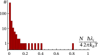
Figure 8: Spectrum of Lyapunov exponents $\{\lambda_{i}\}$ in the strong coupling regime $\alpha\gg 1$. Lyapunov exponents are binned in intervals of length $0.02$.

References

- (1) A. I. Larkin and Y. N. Ovchinnikov, J. High Energy Phys. 28, 1200 (1969)
- (2) Y. Sekino and L. Susskind, J. High Energy Phys. 10, 065 (2008)
- (3) S.V. Syzranov, A.V. Gorshkov and V.M. Galitski, arXiv:1709.09296 (2017)
- (4) P. Hayden and J. Preskill, J. High Energy Phys. 09, 120 (2007)
- (5) M. Blake, Phys. Rev. Lett. 117, 091601 (2016)
- (6) M. Blake, Phys. Rev. D 94, 086014 (2016)
- (7) A. A. Patel and S. Sachdev, Proc. Natl. Acad. Sci. 114, 1844 (2017)
- (8) J. Maldacena, S. H. Shenker, and D. J. Stanford, J. High Energy Phys. 08, 106 (2016)
- (9) S. Sachdev and J. Ye, Phys. Rev. Lett. 70, 3339 (1993)
- (10) A. Kitaev, A simple model of quantum holography, Talks at KITP, April 7, 2015 and May 27, 2015.
- (11) J. Maldacena and D. Stanford, Phys. Rev. D 94, 106002 (2016)
- (12) J. Zaanen, Nature 430, 512 (2004)
- (13) S. Sachdev, Quantum Phase Transitions, John Wiley & Sons, Ltd, ISBN: 9780470022184 (2007)
- (14) A. A. Patel, D. Chowdhury, S. Sachdev, and B. Swingle, Phys. Rev. X 7, 031047 (2017)
- (15) Y. Werman, S. A. Kivelson, E. Berg, arXiv:1705.07895 (2017)
- (16) M. Titov, R. V. Gorbachev, B. N. Narozhny, T. Tudorovskiy, M. Schütt, P. M. Ostrovsky, I. V. Gornyi, A. D. Mirlin, M. I. Katsnelson, K. S. Novoselov, A. K. Geim, and L. A. Ponomarenko, Phys. Rev. Lett. 111, 166601 (2013)
- (17) J. Crossno, J. K. Shi, K. Wang, X. Liu, A. Harzheim, A. Lucas, S. Sachdev, P. Kim, T. Taniguchi, K. Watanabe, T. A. Ohki, and K. C. Fong, Science 351, 1058 (2016)
- (18) H. Guo, E. Ilseven, G. Falkovich, and L. S. Levitov, Proc. Natl. Acad. Sci. 114, 3068 (2017)
- (19) R. Krishna Kumar, D. A. Bandurin, F. M. D. Pellegrino, Y. Cao, A. Principi, H. Guo, G. H. Auton, M. B. Shalom, L. A. Ponomarenko, G. Falkovich, I. V. Grigorieva, L. S. Levitov, M. Polini, and A. K. Geim, Nature Physics 13, 1182 (2017)
- (20) D. A. Bandurin, I. Torre, R. Krishna Kumar, M. Ben Shalom, A. Tomadin, A. Principi, G. H. Auton, E. Khestanova, K. S. Novoselov, I. V. Grigorieva1, L. A. Ponomarenko, A. K. Geim, and M. Polini, Science 351, 1055 (2016)
- (21) L. S. Levitov and G. Falkovich, Nature Phys. 12, 672 (2016)
- (22) U. Briskot, M. Schütt, I. V. Gornyi, M. Titov, B. N. Narozhny, and A. D. Mirlin, Phys. Rev. B 92, 115426 (2015)
- (23) B. N. Narozhny, I. V. Gornyi, A. D. Mirlin, and J. Schmalian, Ann. Phys. 529, 1700043 (2017)
- (24) M. Schütt, P. M. Ostrovsky, I. V. Gornyi, and A. D. Mirlin, Phys.Rev. B 83, 155441 (2011)
- (25) D. T. Son, Phys. Rev. B 75, 235423 (2007)
- (26) D. Chowdhury and B. Swingle, Phys. Rev. D 96, 065005 (2017)
- (27) J. M. Link, B. N. Narozhny, E. I. Kiselev, and J. Schmalian, arXiv:1708.02759 (2017)
- (28) L. Fritz, J. Schmalian, M. Müller, and S. Sachdev, Phys. Rev. B 78, 085416 (2008)
- (29) A. B. Kashuba, Phys. Rev. B 78, 085415 (2008)
- (30) M. Müller, J. Schmalian, and L. Fritz, Phys. Rev. Lett. 103, 025301 (2009)
- (31) I. L. Aleiner, L. Faoro, and L. B. Ioffe, Annals of Physics 375, 378 (2016)
- (32) S. Grozdanov, K. Schalm, and V. Scopelliti, arXiv:1804.09182 (2018)
- (33) M. S. Foster and I. L. Aleiner, Phys. Rev. B 77, 195413 (2008)
- (34) D. C. Elias, R. V. Gorbachev, A. S. Mayorov, S. V. Mo- rozov, A. A. Zhukov, P. Blake, L. A. Ponomarenko, I. V. Grigorieva, K. S. Novoselov, F. Guinea, and A. K. Geim, Nat. Phys. 7, 701 (2011)
- (35) D. A. Siegel, C.-H. Park, C. Hwang, J. Deslippe, A. V. Fedorov, S. G. Louie, and A. Lanzara, Proc. Natl. Acad. Sci. 108, 11365 (2011)
- (36) G. L. Yu, R. Jalil, B. Belle, A. S. Mayorov, P. Blake, F. Schedin, S. V. Morozov, L. A. Ponomarenko, F. Chiappini, S. Wiedmann, U. Zeitler, M. I. Katsnelson, A. K. Geim, K. S. Novoselov, and D. C. Elias, Proc. Natl. Acad. Sci. 110, 3282 (2013)
- (37) D. E. Sheehy and J. Schmalian, Phys. Rev. Lett. 99, 226803 (2007)
- (38) S. H. Shenker, and D. Stanford, J. High Energy Phys. 03, 067 (2014)
- (39) D. Stanford, J. High Energ. Phys. 10, 9 (2016)
- (40) A. Kamenev, Field Theory of Non-Equilibrium Systems, Cambridge University Press, ISBN: 9780521760829 (2011)
- (41) P. Wölfle, Rep. Prog. Phys. 81, 032501 (2018)