Merging $K$-means with hierarchical clustering for identifying general-shaped groups

Abstract

Clustering partitions a dataset such that observations placed together in a group are similar but different from those in other groups. Hierarchical and $K$-means clustering are two approaches but have different strengths and weaknesses. For instance, hierarchical clustering identifies groups in a tree-like structure but suffers from computational complexity in large datasets while $K$-means clustering is efficient but designed to identify homogeneous spherically-shaped clusters. We present a hybrid non-parametric clustering approach that amalgamates the two methods to identify general-shaped clusters and that can be applied to larger datasets. Specifically, we first partition the dataset into spherical groups using $K$-means. We next merge these groups using hierarchical methods with a data-driven distance measure as a stopping criterion. Our proposal has the potential to reveal groups with general shapes and structure in a dataset. We demonstrate good performance on several simulated and real datasets.

1 Introduction

Clustering partitions a dataset into subsets called clusters without any prior knowledge of group assignment. The general objective is that observations placed in the same cluster are similar in some sense while being different to those in other groups. The substantial body of literature (Everitt et al., 2001; Fraley & Raftery, 2002; Hartigan, 1985; Kaufman & Rousseuw, 1990; Kettenring, 2006; Melnykov & Maitra, 2011; McLachlan & Basford, 1988; Murtagh, 1985; Ramey, 1985) dedicated to the topic reflects the difficulty and diversity of clustering applications. Most unsupervised clustering techniques are broadly hierarchical or partition-optimization-based. Traditionally, hierarchical algorithms provide a tree-like structure for demarcating groups, with the property that all observations in a group at some branch are also in the same group higher up the tree. Hierarchical algorithms may be agglomerative (cluster-merging) or divisive (cluster-breaking). Agglomerative algorithms successively merge smaller clusters together whereas divisive algorithms successively break larger clusters apart. Most hierarchical clustering methods use some dissimilarity measure between groups to decide whether to merge (or split) groups. The result can be represented as a dendrogram that can visually express the data structure. Generally, a linkage criteria specifies the dissimilarity between each branch of the dendrogram as a function of the pairwise distances of observations in the sets. The linkage criterion can influence cluster shapes: for example, single linkage is commonly associated with stringy groups while Ward’s linkage is more commonly used for spherical clusters (Johnson & Wichern, 2007). Although the nesting structure provides a broad understanding of the relationships between observations within a dataset, clusters lose homogeneity at higher branches of the tree. Further, hierarchical clustering requires calculating all pairwise distances between observations which is computationally expensive in processor speed (and, more so, in memory) for larger datasets.

Partitional clustering, on the other hand, directly divides a dataset into groups, so that the data in each subset (ideally) share some common trait. Typically the algorithm involves minimizing some measure of dissimilarity between observations within each cluster, while maximizing the dissimilarity between observations in different clusters. The $K$-means algorithm is a very popular choice even though more formal approaches are provided by model-based clustering (Fraley & Raftery, 2002; McLachlan & Peel, 2000; Melnykov & Maitra, 2011). The $K$-means algorithms minimizes the within group sum-of-squares and can be implemented efficiently (Hartigan & Wong, 1979). But $K$-means requires the number of groups ($K$) to be provided or alternatively decided from the data (Maitra et al., 2012). Further, different initialization strategies often produce strikingly different groupings. Also, the algorithm is not as successful with groups that do not have the same and spherical dispersion structure.

(a) $K$-means, $K$ = 2

(b) $K$-means, $K$ = 6

(c) HC, $K$ = 2, single linkage

Figure 1: Partition (using both color and symbol) of the Bullseye dataset with (a) 2-means, (b) 6-means and (c) single linkage hierarchical clustering with 2 groups.

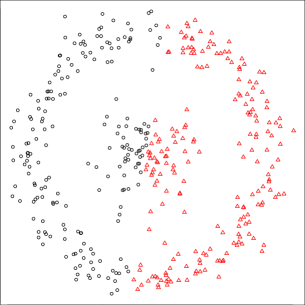
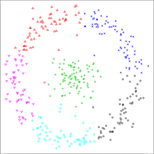
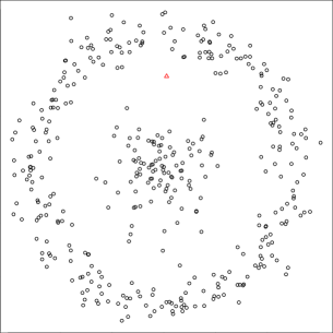
We illustrate some shortcomings of these algorithms through the Bullseye dataset of Stuetzle & Nugent (2010) which has 400 observations from a spherical cluster surrounded by a ring of observations (which form the second group). Figure 1(a-b) shows the clustering using 2- and $6$-means. In addition, Figure 1(c) shows the grouping based on hierarchical clustering with single linkage and $K$ = 2. Neither approach clusters into their true groupings. Although Figure 1(b) captures the center group, we required 5 groups to create the outer ring. One possibility of improving this solution is to merge these groups using some objective mechanism and we will explore this approach in this paper.

The idea of merging clusters is not new in the literature. Fred & Jain (2005) introduced evidence accumulation clustering (EAC) for combining the results from multiple applications of $K$-means. The idea behind EAC is that each partition gives independent evidence on the organization of the data. The authors proposed independent runs of $K$-means on the dataset and created a similarity (frequency) matrix between all pairs of data points with the $(i,j)$th entry representing the number of times the $i$th and $j$th observations were placed in the same group. The final data partition is obtained by applying a hierarchical agglomerative clustering algorithm using this similarity matrix. The motivation here is that observations that are together in the majority of partitions should also be so in the final chosen partition. This procedure is novel in that it chooses among several different partitions but it is computationally expensive since it involves performing either single linkage or average linkage on an $n\times n$ distance matrix, where $n$ is the number of observations. Stuetzle & Nugent (2010) adopt a nonparametric approach to clustering based on the premise that groups correspond to modes of the density. Stuetzle & Nugent (2010) find the modes within a dataset and assign observations to the “domain of attraction" of a mode. The collection of high density modes is used to create a hierarchical structure where dissimilarity between modes is based on the lowest density observed between any pair of groups. Baudry et al. (2010) propose a cluster merging method using a model-based clustering approach. They propose first selecting the total number of Gaussian mixtures components, $K_{0}$, using BIC and then combining them hierarchically. This yields a unique soft clustering for each $K$ less than $K_{0}$. Further refinements to this method were provided by the DEMP (Hennig, 2010) and DEMP+ (Melnykov, 2016) algorithms. However, model-based clustering is computationally slower and typically more difficult to apply on to larger datasets.

In this paper, we propose a $K$-means hierarchical ($K-mH$) cluster merging algorithm which combines the computational benefits of $K$-means with agglomerative hierarchical clustering. The general methodology and our algorithm are detailed in Section 2. We present several examples of datasets with clusters of complicated/general shapes in Section 3 to illustrate and evaluate our algorithm. We end with a short discussion.

2 Methodology

Let ${\mathcal{S}}=\{{\mathbf{X}}_{1},{\mathbf{X}}_{2},\ldots,{\mathbf{X}}_{n}\}$ be a dataset of $n$ $p$-dimensional observations that are presumed to be in a partition $P$ comprising defined categories ${\mathcal{C}}_{1},{\mathcal{C}}_{2},\ldots,{\mathcal{C}}_{K}$ according to some similarity measure between observations. Suppose we have $N$ such partitions of a dataset ${\mathcal{S}}$ where $\Psi=\{P^{1},P^{2},\ldots,P^{N}\}$ is the set of the $N$ partitions. Then we define $P^{i}=\{{\mathcal{C}}^{i}_{1},{\mathcal{C}}^{i}_{2},\ldots,{\mathcal{C}}^{i}_{K_{i}}\}$ as a candidate partition where ${\mathcal{C}}^{i}_{j}$ is cluster $j$ of partition $P^{i}$, $|{\mathcal{C}}^{i}_{j}|$ is the number of observations in ${\mathcal{C}}^{i}_{j}$, $K_{i}$ is the number of clusters in partition $P^{i}$ and $\sum_{j=1}^{K_{i}}|{\mathcal{C}}^{i}_{j}|=n$ for all $i$. Then the goal is to find, among the $N$ partitions in $\Psi$, the optimal partition $P_{*}$ that ideally provides a close match to the true partition. Our objective in this paper is to provide methodology to identify the partitions $P_{i}$ and the optimal $P_{*}$.

2.1 Background and Preliminaries

The development of our algorithm borrows ideas from $K$-means and hierarchical clustering, so we revisit them briefly.

2.1.1 $K$-means:

The $K$-means algorithm starts with $K_{0}$ $p$-dimensional seeds $\{{\mbox{\boldmath${\mu}$}}^{(0)}_{k};1\leq k\leq K_{0}\}$ and then iterates between cluster assignments and mean updates till convergence. Therefore, at the $i$th step, we update our partitions to be ${\mathcal{C}}_{k}^{(i)}=\{{\mathbf{X}}_{j}\text{ : }\|{\mathbf{X}}_{j}-{\mbox{\boldmath${\mu}$}}^{(i)}_{k}\|\ =\min\limits_{1\leq l\leq K}\|{\mathbf{X}}_{j}-{\mbox{\boldmath${\mu}$}}^{(l)}_{k}\|j=1,\ldots,n\}$, for $k=1,2,\ldots,K_{0}$, with $\|x\|=\sqrt{x^{\prime}x}$. These updates are followed by recalculated cluster means, with ${\mbox{\boldmath${\mu}$}}^{(i+1)}_{k}=\sum_{j\in{\mathcal{C}}_{k}^{(i)}}{\mathbf{X}}_{j}/{|{\mathcal{C}}_{k}^{(i)}|}$. The algorithm continues until there are no further changes in $\{{\mathcal{C}}_{k}^{(i)}:k=1,\ldots,K_{0}\}$ (or, equivalently, in the ${\mbox{\boldmath${\mu}$}}^{(i)}_{k}$s).

Initialization:

Initialization can greatly impact performance of $K$-means (Maitra, 2009) so we adopt MacQueen (1967)’s suggestion that samples $K$ distinct observations from the dataset as initial seeds and runs the algorithm to convergence. We run this procedure $I$ times, with the converged solution having the smallest within-group sum-of-squares chosen as our $K$-groups partition. This approach is the default setting of the kmeans() function in R (R Core Team, 2017), with the number of initializations set by the nstart argument.

Choosing $K_{0}$:

Many methods (for example, Marriott, 1971; Tibshirani et al., 2003; McLachlan, 1987; Sugar & James, 2003; Maitra et al., 2012) exist for choosing $K_{0}$. Here we discuss the Krzanowski & Lai (1988) criterion which uses the trace of the pooled within-group variance-covariance matrix, which we denote as $W_{g}$ for a $K$-groups partition. Following Krzanowski & Lai (1988), $trace(W_{K})$ should decrease dramatically as $K$ increases provided that $K<\tilde{K}$, where $\tilde{K}$ is the true number of spherical groups, but that this decrease should slow down once $K\geq\tilde{K}$. Based on this rationale, and defining $Diff(K)=(K-1)^{2/p}trace(W_{K-1})-K^{2/p}trace(W_{K})$, the number of homogeneous spherically-dispersed groups $K_{0}$ can be obtained as follows: Let $C_{K}=|Diff(K)/Diff(K+1)|$ and $K_{1},K_{2},\ldots,K_{l}$ be such that $C_{K_{1}}\geq C_{K_{2}}\geq,\ldots,\geq C_{K_{l}}$. Then choose $K_{0}=K_{1}$.

2.1.2 Agglomerative Hierarchical clustering:

Here, we successively merge current groups assuming a distance $d(A,B)$ between any two groups $A$ and $B$ and a mechanism (or linkage) to recalculate the distances when groups are merged. Examples of linkages are single where $d(A,B)=\min\{\|x-y\|:x\in A,y\in B\}$ or average with $d(A,B)=\sum_{x\in A}\sum_{y\in B}\|x-y\|/(|A||B|)$. The algorithm initially places every observation in its own group, that is, by setting $\tilde{{\mathcal{C}}_{j}}^{(0)}={\mathbf{X}}_{j}$ for all $j=1,2,\ldots,n$. Then, we successively merge clusters at each stage, so that at the $i$th stage, we have $n-i$ clusters, with $(n-i-2)$ many of those groups unchanged from the previous stage. That is, we have $\tilde{{\mathcal{C}}}_{j}^{(i)}\equiv\tilde{{\mathcal{C}}}_{j}^{(i-1)}$ for all $j\in\{1,\ldots,n-i\}\setminus(k.l)$ where $k,l$ are such that $k<l$ and $d(\tilde{{\mathcal{C}}}_{k}^{i-1},\tilde{{\mathcal{C}}}_{l}^{i-1})=\min_{1\leq m<q\leq n-i+1}{d(\tilde{{\mathcal{C}}_{m}}^{(i-1)},\tilde{{\mathcal{C}}}_{q}^{(i-1)})}$. Set $\tilde{{\mathcal{C}}}_{k}^{(i)}=\tilde{{\mathcal{C}}}_{k}^{(i-1)}\cup\tilde{{\mathcal{C}}}_{l}^{(i-1)}$ and if $l<n-i+1$ then $\tilde{{\mathcal{C}}}_{l}^{(i)}=\tilde{{\mathcal{C}}}_{n-i+1}^{(i-1)}$. Set $i$ = $i+1$. The merging continues until the entire hierarchy has been built, or a hierarchy with a pre-specified number of groups $K_{\bullet}$ have been obtained.

2.2 The $K$-means hierarchical ($K$-mH) cluster merging algorithm

Our proposed algorithm removes scatter and then creates multiple partitions, each formed by combining $K$-means and hierarchical clustering. The algorithm has the following steps.

1. Removing scatter from the dataset: The algorithm first removes scatter from the dataset from consideration.

2. Finding a partition: Our algorithm has two phases. The first focuses on finding a (potentially) large number ($K_{0}$) of homogeneous spherical groups while the next merges these groups according to some criterion. We call these phases the $K$-means and hierarchical phases. The exact details of these phases are as follows:

   1. The $K$-means phase: For a given $K_{0}$ and initialization, the $K$-means phase uses its namesake algorithm with multiple ($m$) initializations to identify $K_{0}$ homogeneous spherically-distributed groups. This phase yields $K_{0}$ groups $\{{\mathcal{C}}_{1},{\mathcal{C}}_{2},\ldots,{\mathcal{C}}_{K_{0}}\}$ with means ${\mbox{\boldmath${\mu}$}}_{1},{\mbox{\boldmath${\mu}$}}_{2},\ldots,{\mbox{\boldmath${\mu}$}}_{K_{0}}$. Each obtained cluster ${\mathcal{C}}_{k}$ is now considered to be one entity. Therefore, we now have $K_{0}$ entities labeled as ${{\mathcal{C}}_{1}},{\mathcal{C}}_{2},\ldots,{{\mathcal{C}}_{K_{0}}}$ for consideration.

   2. Hierarchical phase: For given $K_{*}$ and distance $d(\cdot,\cdot)$, we successively merge the $K$-means groups as follows:

      1. Set $i^{*}=1$ and $d^{*}_{1}=1$. Define $\tilde{{\mathcal{C}}_{j}}^{(1)}={\mathcal{C}}_{j}$ for all $j$.

      2. For $j\in 1...(K_{0}-i^{*})$ $\tilde{{\mathcal{C}}}_{j}^{(i^{*}+1)}=\tilde{{\mathcal{C}}}_{j}^{(i^{*})}$. Find $k,l$ such that $k<l$ and $d(\tilde{{\mathcal{C}}}_{k}^{i^{*}},\tilde{{\mathcal{C}}}_{l}^{i^{*}})=\min_{1\leq m<q\leq(K_{0}-i^{*}+1)}{d(\tilde{{\mathcal{C}}}_{m}^{i^{*}},\tilde{{\mathcal{C}}}_{q}^{i^{*}})}$. Set $\tilde{{\mathcal{C}}}_{k}^{(i^{*}+1)}=\tilde{{\mathcal{C}}}_{k}^{(i^{*})}\cup\tilde{{\mathcal{C}}}_{l}^{(i^{*})}$ and if $l<K_{0}-i^{*}+1$ then $\tilde{{\mathcal{C}}}_{l}^{(i^{*}+1)}=\tilde{{\mathcal{C}}}_{K_{0}-i^{*}+1}^{(i^{*})}$, define $d^{*}_{i^{*}}=d(\tilde{{\mathcal{C}}}_{k}^{i^{*}},\tilde{{\mathcal{C}}}_{l}^{i^{*}})$. Set $i^{*}$ = $i^{*}+1$.

      3. If $i^{*}=K_{0}$ or $i^{*}=K_{0}-K_{*}+1$ terminate, else return to Step 2(b).

3. Forming multiple partitions and choosing the optimal $P_{*}$: Repeat Step 2 $N=ML$ times with $M$ different $K_{0}$s and $L$ different $K_{*}$s to form multiple partitions. Determine the optimal hierarchical partition $P_{*}$.

Our outlined algorithm has several aspects that need clarification. We do this next.

2.2.1 Scatter Removal:

Outliers or scatter can greatly influence clustering performance (Maitra & Ramler, 2009). Although many methods (Byers & Raftery, 1998; Tseng & Wong, 2005; Maitra & Ramler, 2009) exist, we adopt the following straightforward approach to eliminating scatter. We use $K$-means with the largest of our candidate group sizes ($G$) and multiple initializations ($K\sqrt{np}$) to obtain a $G$-means partition. Observations in any of the $G$ groups that have less than 0.1% of the size of the dataset are labeled as scatter and eliminated from further consideration. This leaves us with $n^{*}$ observations ${\mathbf{X}}_{1},{\mathbf{X}}_{2},\ldots,{\mathbf{X}}_{n^{*}}$ (say) which we proceed with clustering using $K-mH$.

2.2.2 Distance between entities:

For the hierarchical phase of Step 2, we calculate the distance between two clusters obtained from the $K$-means step by assuming (non-homogeneous) spherically-dispersed Gaussian-distributed groups in the dataset. Specifically, we let ${\mathbf{X}}_{1},{\mathbf{X}}_{2},\ldots,{\mathbf{X}}_{n^{*}}$ be independent $p$-variate observations with ${\mathbf{X}}_{i}\sim N_{p}({\mbox{\boldmath${\mu}$}}_{\zeta_{i}},\sigma^{2}_{\zeta_{i}}{\bf I})$, where $\zeta_{i}\in\{1,2,\ldots,K\}$ for $i=1,2,\ldots,n^{*}$. Here we assume that ${\mbox{\boldmath${\mu}$}}_{k}$’s are all distinct and that $n_{k}$ is the number of observations in cluster $k$. Then the density for the ${\mathbf{X}}_{i}$’s is given by $f({\mathbf{X}})=\sum_{k=1}^{K}{I({\mathbf{X}}\in{{\mathcal{C}}}_{k})\phi({\mathbf{X}};{\mbox{\boldmath${\mu}$}}_{k},\sigma^{2}_{k}\text{I})},$ where $\mathcal{C}_{k}$ is a cluster indexed by the $N_{p}({\mbox{\boldmath${\mu}$}}_{k},\sigma^{2}_{k}{\bf I})$ density and $I({\mathbf{X}}\in{{\mathcal{C}}}_{k})$ is an indicator function specifying whether observation ${\mathbf{X}}$ belongs to the $kth$ group having a $p$-dimensional multivariate normal density $\phi({\mathbf{X}};{\mbox{\boldmath${\mu}$}}_{k},\sigma^{2}_{k}{\bf I})\propto\sigma_{k}^{-p}\exp\left[-\frac{1}{2\sigma_{k}^{2}}({\mathbf{X}}-{\mbox{\boldmath${\mu}$}}_{k})^{\prime}({\mathbf{X}}-{\mbox{\boldmath${\mu}$}}_{k})\right]$, $k=1,\ldots,K$. Define the distance measure

$$\mathcal{D}_{k}({\mathbf{X}}_{i})=\frac{({\mathbf{X}}_{i}-{\mbox{\boldmath${\mu}$}}_{k})^{\prime}({\mathbf{X}}_{i}-{\mbox{\boldmath${\mu}$}}_{k})}{\sigma_{k}^{2}}$$ (1)

and the variable

$$Y^{j,l}({\mathbf{X}})\;{=}\;\mathcal{D}_{j}({{\mathbf{X}}})-\mathcal{D}_{l}({{\mathbf{X}}}),\;\textup{ where }{{\mathbf{X}}}\in{{\mathcal{C}}}_{l},$$ (2)

and $Y^{l,j}({\mathbf{X}})$ similarly. Using the spherically-dispersed Gaussian models formulated above, $Y^{j,l}({\mathbf{X}})$ is a random variable which represents the difference in squared distances of ${\mathbf{X}}\in{\mathcal{C}}_{l}$ to the center of ${{\mathcal{C}}}_{j}$ and to the center of ${{\mathcal{C}}}_{l}$. Then $p^{j}_{l}=\Pr[Y^{j,l}({\mathbf{X}})<0]$ is the probability that an observation from ${\mathcal{C}}_{l}$ is classified into ${{\mathcal{C}}}_{j}$ and is calculated as follows.

Theorem 1.

Let ${\mathbf{X}}\sim N_{p}({\mbox{\boldmath${\mu}$}}_{l},{\mathbf{\Sigma}}_{l})$, with ${\mathbf{\Sigma}}_{l}$ a positive-definite matrix. Further, let $Y^{j,l}({\mathbf{X}})={\mathcal{D}}_{j}({\mathbf{X}})-{\mathcal{D}}_{l}({\mathbf{X}})$, where ${\mathcal{D}}_{k}({\mathbf{X}})=({\mathbf{X}}-{\mbox{\boldmath${\mu}$}}_{k})^{\prime}{\mathbf{\Sigma}}_{k}^{-1}({\mathbf{X}}-{\mbox{\boldmath${\mu}$}}_{k})$ for $k\in\{j,l\}$. Let $\lambda_{1},\lambda_{2},\ldots,\lambda_{p}$ be the eigenvalues of ${\mathbf{\Sigma}}_{j|l}\equiv{\mathbf{\Sigma}}_{l}^{\frac{1}{2}}{\mathbf{\Sigma}}_{j}^{-1}{\mathbf{\Sigma}}_{l}^{\frac{1}{2}}$ with corresponding eigenvectors ${\mbox{\boldmath${\gamma}$}}_{1},{\mbox{\boldmath${\gamma}$}}_{2},...{\mbox{\boldmath${\gamma}$}}_{p}$. Then $Y^{j,l}({\mathbf{X}})$ is distributed as $\sum^{p}_{i=1}I(\lambda_{i}\neq 1)\left[(\lambda_{i}-1)U_{i}-\lambda_{i}\delta_{i}^{2}/(\lambda_{i}-1)\right]+\sum^{p}_{i=1}I(\lambda_{i}=1)\delta_{i}(2Z_{i}+\delta_{i}),$ where $U_{i}^{\prime}s$ are independent non-central $\chi^{2}$ random variables with one degree of freedom and non-centrality parameter $\lambda_{i}^{2}\delta_{i}^{2}/(\lambda_{i}-1)^{2}$ with $\delta_{i}={\mbox{\boldmath${\gamma}$}}_{i}^{\prime}{\mathbf{\Sigma}}_{l}^{-\frac{1}{2}}({\mbox{\boldmath${\mu}$}}_{l}-{\mbox{\boldmath${\mu}$}}_{j})$ for $i\in\{1,2,...,p\}\cap\{i:\lambda_{l}\neq 1\}$, independent of $Z_{i}$’s, which are independent standard normal random variables, for $i\in\{1,2,...,p\}\cap\{i:\lambda_{i}=1\}.$

Proof.

Let ${\mbox{\boldmath${\xi}$}}\sim N_{p}(0,{{\bf I}})$. Since ${\mathbf{X}}\stackrel{{\scriptstyle d}}{{=}}{\mathbf{\Sigma}}_{l}^{\frac{1}{2}}{\mbox{\boldmath${\xi}$}}+{\mbox{\boldmath${\mu}$}}_{l}$, we have

$$Y^{j,l}({\mathbf{X}}) {=} {{\mathbf{X}}}^{\prime}({\mathbf{\Sigma}}_{j}^{-1}-{\mathbf{\Sigma}}_{l}^{-1}){{\mathbf{X}}}+2{{\mathbf{X}}}^{\prime}({\mathbf{\Sigma}}_{l}^{-1}{\mbox{\boldmath${\mu}$}}_{l}-{\mathbf{\Sigma}}_{j}^{-1}{\mbox{\boldmath${\mu}$}}_{j})+{\mbox{\boldmath${\mu}$}}_{j}^{\prime}{\mathbf{\Sigma}}_{j}^{-1}{\mbox{\boldmath${\mu}$}}_{j}-{\mbox{\boldmath${\mu}$}}_{l}^{\prime}{\mathbf{\Sigma}}_{l}^{-1}{\mbox{\boldmath${\mu}$}}_{l}$$ (3)

$$\stackrel{{\scriptstyle d}}{{=}} ({\mathbf{\Sigma}}_{l}^{\frac{1}{2}}{\mbox{\boldmath${\xi}$}}+{\mbox{\boldmath${\mu}$}}_{l})^{\prime}({\mathbf{\Sigma}}_{j}^{-1}-{\mathbf{\Sigma}}_{l}^{-1})({\mathbf{\Sigma}}_{l}^{\frac{1}{2}}{\mbox{\boldmath${\xi}$}}+{\mbox{\boldmath${\mu}$}}_{l})+2({\mathbf{\Sigma}}_{l}^{\frac{1}{2}}{\mbox{\boldmath${\xi}$}}+{\mbox{\boldmath${\mu}$}}_{l})^{\prime}({\mathbf{\Sigma}}_{l}^{-1}{\mbox{\boldmath${\mu}$}}_{l}-{\mathbf{\Sigma}}_{j}^{-1}{\mbox{\boldmath${\mu}$}}_{j})+{\mbox{\boldmath${\mu}$}}_{j}^{\prime}{\mathbf{\Sigma}}_{j}^{-1}{\mbox{\boldmath${\mu}$}}_{j}-{\mbox{\boldmath${\mu}$}}_{l}^{\prime}{\mathbf{\Sigma}}_{l}^{-1}{\mbox{\boldmath${\mu}$}}_{l}$$

$$= {\mbox{\boldmath${\xi}$}}^{\prime}({\mathbf{\Sigma}}_{j|l}-{{\bf I}}){\mbox{\boldmath${\xi}$}}+2{\mbox{\boldmath${\xi}$}}^{\prime}{\mathbf{\Sigma}}_{l}^{\frac{1}{2}}{\mathbf{\Sigma}}_{j}^{-1}({\mbox{\boldmath${\mu}$}}_{l}-{\mbox{\boldmath${\mu}$}}_{j})+({\mbox{\boldmath${\mu}$}}_{l}-{\mbox{\boldmath${\mu}$}}_{j})^{\prime}({\mathbf{\Sigma}}_{j}^{-1})({\mbox{\boldmath${\mu}$}}_{l}-{\mbox{\boldmath${\mu}$}}_{j})$$

where ${\mathbf{\Sigma}}_{j|l}={\mathbf{\Sigma}}_{l}^{\frac{1}{2}}{\mathbf{\Sigma}}_{j}^{-1}{\mathbf{\Sigma}}_{l}^{\frac{1}{2}}$. Let the spectral decomposition of ${\mathbf{\Sigma}}_{j|l}$ be given by ${\mathbf{\Sigma}}_{j|l}={\mathbf{\Gamma}}_{j|l}{\mathbf{\Lambda}}_{j|l}{\mathbf{\Gamma}}^{\prime}_{j|l}$, where ${\mathbf{\Lambda}}_{j|l}$ is a diagonal matrix containing the eigenvalues $\lambda_{1},\lambda_{2},\ldots\lambda_{p}$ of ${\mathbf{\Sigma}}_{j|l}$, and ${\mathbf{\Gamma}}_{j|l}$ is an orthogonal matrix containing the eigenvectors ${\mbox{\boldmath${\gamma}$}}_{1},{\mbox{\boldmath${\gamma}$}}_{2},\ldots,{\mbox{\boldmath${\gamma}$}}_{p}$ of ${\mathbf{\Sigma}}_{j|l}$. Since $\mathbf{Z}\equiv{{\mathbf{\Gamma}}_{j|l}}^{\prime}{\mbox{\boldmath${\xi}$}}\sim N_{p}(0,{{\bf I}})$ as well, we get from (3) that

$$Y^{j,l}({\mathbf{X}}) \stackrel{{\scriptstyle d}}{{=}} {\mbox{\boldmath${\xi}$}}^{\prime}({\mathbf{\Gamma}}_{j|l}{\mathbf{\Lambda}}_{j|l}{\mathbf{\Gamma}}^{\prime}_{j|l}-{\mathbf{\Gamma}}_{j|l}{\mathbf{\Gamma}}^{\prime}_{j|l}){\mbox{\boldmath${\xi}$}}+2{\mbox{\boldmath${\xi}$}}^{\prime}({\mathbf{\Gamma}}_{j|l}{\mathbf{\Lambda}}_{j|l}{\mathbf{\Gamma}}^{\prime}_{j|l}{\mathbf{\Sigma}}^{-\frac{1}{2}}_{1})({\mbox{\boldmath${\mu}$}}_{l}-{\mbox{\boldmath${\mu}$}}_{j})+({\mbox{\boldmath${\mu}$}}_{l}-{\mbox{\boldmath${\mu}$}}_{j})^{\prime}({\mathbf{\Sigma}}^{-\frac{1}{2}}_{1}{\mathbf{\Gamma}}_{j|l}{\mathbf{\Lambda}}_{j|l}{\mathbf{\Gamma}}^{\prime}_{j|l}{\mathbf{\Sigma}}^{-\frac{1}{2}}_{l})({\mbox{\boldmath${\mu}$}}_{l}-{\mbox{\boldmath${\mu}$}}_{j})$$ (4)

$$= ({\mathbf{\Gamma}}^{\prime}_{j|l}{\mbox{\boldmath${\xi}$}})^{\prime}({\mathbf{\Lambda}}_{j|l}-{{\bf I}})({\mathbf{\Gamma}}^{\prime}_{j|l}{\mbox{\boldmath${\xi}$}})+2({\mathbf{\Gamma}}^{\prime}_{j|l}{\mbox{\boldmath${\xi}$}})^{\prime}({\mathbf{\Lambda}}_{j|l}{\mathbf{\Gamma}}_{j|l}{\mathbf{\Sigma}}^{-\frac{1}{2}}_{l})({\mbox{\boldmath${\mu}$}}_{l}-{\mbox{\boldmath${\mu}$}}_{j})+({\mbox{\boldmath${\mu}$}}_{l}-{\mbox{\boldmath${\mu}$}}_{j})^{\prime}({\mathbf{\Sigma}}^{-\frac{1}{2}}_{l}{\mathbf{\Gamma}}_{j|l}{\mathbf{\Lambda}}_{j|l}{\mathbf{\Gamma}}_{j|l}^{\prime}{\mathbf{\Sigma}}^{-\frac{1}{2}}_{l})({\mbox{\boldmath${\mu}$}}_{l}-{\mbox{\boldmath${\mu}$}}_{j})$$

$$\stackrel{{\scriptstyle d}}{{=}} \sum_{i=1}^{p}\left[(\lambda_{i}-1){Z_{i}}^{2}+2\lambda_{i}\delta_{i}Z_{i}+\lambda_{i}\delta_{i}^{2}\right],$$

where $\delta_{i},i=1,2,\ldots,p$ are as in the statement of the theorem. We can simplify (4) further based on the values of $\lambda_{i}$: If $\lambda_{i}>1$: $(\lambda_{i}-1)Z_{i}^{2}+2\lambda_{i}\delta_{i}Z_{i}+\lambda_{i}\delta_{i}^{2}=(\sqrt{\lambda_{i}-1}Z_{i}+\lambda_{i}\delta_{i}/\sqrt{\lambda_{i}-1})^{2}-\lambda_{i}\delta_{i}^{2}/(\lambda_{i}-1)$, while for $\lambda_{i}<1$: $(\lambda_{i}-1){Z_{i}}^{2}+2\lambda_{i}\delta_{i}Z_{i}+\lambda_{i}\delta_{i}^{2}=-(\sqrt{1-\lambda_{i}}Z_{i}-\lambda_{i}\delta_{i}/\sqrt{1-\lambda_{i}})^{2}-\lambda_{i}\delta_{i}^{2}/(\lambda_{i}-1)$. In both cases, $(\lambda_{i}-1){Z_{i}}^{2}+2\lambda_{i}\delta_{i}Z_{i}+\lambda_{i}\delta_{i}^{2}$ is distributed as a $(\lambda_{i}-1)\chi^{2}_{l,\lambda^{2}_{i}\delta^{2}_{i}/(\lambda_{i}-1)^{2}}$-random variable shifted by $-\lambda_{i}\delta_{i}^{2}/(\lambda_{i}-1)$. When $\lambda_{i}=1$, $(\lambda_{i}-1)Z_{i}^{2}+2\lambda_{i}\delta_{i}Z_{i}+\lambda_{i}\delta_{i}^{2}=2\delta_{i}Z_{i}+\delta_{i}^{2}.$ The theorem follows from some further minor rearrangement of terms. ∎

Corollary 1.

Let ${\mathbf{X}}\sim N_{p}({\mbox{\boldmath${\mu}$}}_{l},\sigma_{l}^{2}{\bf I})$. Define ${\mathcal{D}}_{k}({\mathbf{X}})$ as in (1). If $\sigma_{l}=\sigma_{j}$, we have $Y^{j,l}({\mathbf{X}})\sim N(\left\lVert{\mbox{\boldmath${\mu}$}}_{j}-{\mbox{\boldmath${\mu}$}}_{l}\right\rVert^{2}/\sigma_{l}^{2},4\left\lVert{\mbox{\boldmath${\mu}$}}_{j}-{\mbox{\boldmath${\mu}$}}_{l}\right\rVert^{2}/\sigma_{l}^{2})$, otherwise $Y^{j,l}({\mathbf{X}})\sim(\sigma_{l}^{2}/\sigma_{j}^{2}-1)\chi^{2}_{p;\left\lVert{\mbox{\boldmath${\mu}$}}_{l}-{\mbox{\boldmath${\mu}$}}_{j}\right\rVert^{2}/{(\sigma_{j}^{2}-\sigma_{l}^{2})}^{2}}-\left\lVert{\mbox{\boldmath${\mu}$}}_{l}-{\mbox{\boldmath${\mu}$}}_{j}\right\rVert^{2}/(\sigma_{l}^{2}-\sigma_{j}^{2})$.

Proof.

Here, $\lambda_{i}\equiv\sigma_{l}^{2}/\sigma_{j}^{2}$, ${\mbox{\boldmath${\gamma}$}}_{i}$ is the $i$th unit vector, and $\sum_{i=1}^{p}\delta_{i}^{2}=\left\lVert\mu_{l}-\mu_{j}\right\rVert^{2}/\sigma_{l}^{2}$. Also, the sum of $p$ independent $\chi^{2}_{1;\tau_{i}^{2}}$ random variables has the same distribution as a $\chi^{2}_{p;\sum_{i=1}^{p}\tau_{i}^{2}}$ random variable. The proof follows from Theorem 1. ∎

Corollary 1 provides an easy calculation for $p^{j}_{l}$ and $p_{j}^{l}$. Note, however, that for large $\delta$ (and/or $p$) the $\chi^{2}_{p;\delta}$ cumulative distribution function is not evaluated accurately so we approximate this quantity by the corresponding cumulative distribution function of the $N(p+\delta,2(p+2\delta))$ random variable (for details, see Muirhead, 2005, pages 22-24 and problem 1.8). The net result is that we have approximate but very speedy and accurate calculations. This is important because our hierarchical phase uses the distance measure between groups ${\mathcal{C}}_{j}$ and ${\mathcal{C}}_{l}$ that we define to be

$$d({\mathcal{C}}_{j},{\mathcal{C}}_{l})=1-(p^{j}_{l}+p^{l}_{j})/2.$$ (5)

We now adapt this distance measure to the initial and iterative parts of the hierarchical phase. At the beginning of the hierarchical phase (equivalently, the conclusion of the $K$-means phase), we have $K_{0}$ entities with labels ${\mathcal{C}}_{1},\ldots,{\mathcal{C}}_{K_{0}}$. For $1\leq k\leq K_{0}$, we already have the $\hat{\mbox{\boldmath${\mu}$}}_{k}$s while the covariance matrix ($\hat{\sigma}^{2}_{k}{\bf I}$) is estimated by setting $\sigma_{k}^{2}$ as the trace of the variance-covariance matrix of ${\mathcal{C}}_{k}$ scaled by $p$. For subsequent stages, (5) is updated by replacing the distance between an entity (say, ${\mathcal{C}}_{l}$) and a merged entity (say, ${\mathcal{C}}_{j}\cup{\mathcal{C}}_{k}$) as $d({\mathcal{C}}_{l},{\mathcal{C}}_{j}\cup{\mathcal{C}}_{k})=\min\{d({\mathcal{C}}_{l},{\mathcal{C}}_{j}),d({\mathcal{C}}_{l},{\mathcal{C}}_{k})\}$. A convenient aspect of this strategy is that off-the-shelf hierarchical clustering software (for example, the hclust function in R) with single linkage can be used to implement the hierarchical phases of our $K$-mH algorithm.

2.2.3 Forming $N$ partitions and choosing $P_{*}$:

Step 2 of the $K-mH$ algorithm produces one partition starting with $K_{0}$ entities ending with $K_{*}$ clusters. Step 3 runs Step 2 $N=ML$ times, where $M$ is the number of $K_{0}$s and $L$ is the number of $K_{*}$s used. We discuss choosing $K_{0}$ and $K_{*}$ next.

Choosing candidate $K_{0}$:

Our proposal for $K_{0}$ involves chooses a range of values $\{k_{1},k_{2},\ldots,k_{m}\}$, $m\geq M$ for which we calculate $C_{k_{1}},C_{k_{2}},\ldots,C_{k_{m}}$ using Krzanowski & Lai (1988)’s suggestions of Section 2.1.1. We sort these values to get $C_{g_{1}}\geq C_{g_{2}}\geq,\ldots,\geq C_{g_{m}}$, where the set $\{g_{1},g_{2},\ldots,g_{m}\}=\{k_{1},k_{2},\ldots,k_{m}\}$. However, instead of setting $K_{0}\equiv g_{1}$ as recommended by Krzanowski & Lai (1988), we propose running Step 2 of our algorithm for each $K_{0}\equiv K_{o}^{(i)}$, where $K_{0}^{(1)}=g_{1},K_{0}^{(2)}=g_{2},\ldots,K_{0}^{(M)}=g_{M}$, that is, for the numbers of clusters corresponding to the $M$ highest $C_{g_{j}}$s. So we run the $K$-means phase $M$ times with $K_{0}=K_{0}^{(i)}$ for $i=1,2,\ldots,M$, with $K_{0}^{(1)}=g_{1},K_{0}^{(2)}=g_{2},\ldots,K_{0}^{(M)}=g_{M}.$ For each of these runs, we set $K_{*}\equiv K_{*}^{(i)}$ in the hierarchical phase and in the manner described next.

Choosing candidate $K_{*}$:

For each value of $K_{0}^{(i)}$, we use $K_{*}$ if the number of desired general-shaped clusters is known and then we set $L=1$. When $K_{*}$ is unknown, we obtain a range of $K_{*}$s by defining change-points ($CP$s) as $CP_{k}=d^{*}_{k+1}-d^{*}_{k}$ (for $k=1,\ldots,K_{0}^{(i)}$) where $d^{*}_{1}\leq d^{*}_{2}\leq\ldots\leq d^{*}_{K_{0}^{(i)}}$ are calculated during Step 2b of the algorithm. We sort these $CP$-values to get $CP_{q_{1}}\geq CP_{q_{2}}\geq,\ldots,\geq CP_{q_{K_{0}^{(i)}-1}}$, where the set $\{q_{1},q_{2},\ldots,q_{K_{0}^{(i)}-1}\}$ is some appropriate permutation of the set $\{2,3,\ldots,K_{o}^{(i)}\}$. We consider the first $L$ of these values. That is, we define $k_{i,1}=q_{1},k_{i,2}=q_{2},\ldots,k_{i,L}=q_{L}$ as in Section 2.2.3 for when we have $K_{0}=K_{0}^{(i)}$. Then for each $K_{0}^{(i)}$ we obtain $L$ partitions using $K_{*}=k_{i,j}$ for $j\in\{1,2,\ldots,L\}.$ Thus, we arrive at $N=ML$ partitions $\{P_{1},P_{2},\ldots,P_{N}\}$ for all combinations of $K_{0}$ and $K_{*}$.

2.2.4 Visualizing partitions and choosing optimal $K_{*}$:

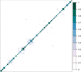
We extend Fred & Jain (2005)’s ideas to visualize the stability and variability in our partitions. Consider the $n\times n$ similarity matrix $\Psi$ with $(i,j)$th entry $\psi_{ij}=n_{i,j}/N$, where $n_{ij}$ is the number of times that the $i$th and $j$th observations are in the same cluster across the $N$ partitions obtained from Section 2.2.3. We display $\Psi$ via a clustered heatmap. The heatmap provides indication into both the structure and stability of the clustering. We can use this heatmap to decide on $K_{*}$ by determining all partitions which remain after thresholding below $\psi_{ij}=0.5$. We use two alternative choices in forming these partitions. In the first case, if the off-diagonal $\psi_{ij}$s are generally small or uncertain (i.e. their mean is small or their coefficient of variation is high), we use single-linkage otherwise we use complete linkage. As with Fred & Jain (2005), heatmaps create very large files for large $n$ so we then use a random sample of the observations. We replicate this process $B$ times to assess the variability in $K_{*}$.

Final partition:

With $K_{*}$ known or determined through the methods of Section 2.2.4, we have $L=1$ as per Section 2.2.3. Then, with the $N=M$ partitions, we pick the clustering that is most similar to the other $N-1$ partitions. This is operationally implemented by defining the $N\times N$ matrix $\mathcal{W}$ where $\mathcal{W}_{i,j}=\mathcal{R}_{i,j}$, where $\mathcal{R}_{i,j}$ is the value for the Adjusted Rand Index (Hubert & Arabie, 1985) between partitions $P_{i}$ and $P_{j}$. Define the objective function: $\bar{\mathcal{W}_{i}}=\sum_{j}{\mathcal{W}_{i,j}/N}.$ Then, we choose $P_{*}$ to be the partition that best matches $\Psi$ in the sense of maximizing the objective function. Thus, $P_{*}=\{P^{i}:\bar{\mathcal{W}_{i}}=\max\limits_{1<j<N}{\bar{\mathcal{W}_{j}}}\}$is our choice for the final clustering and represents the partition that is most similar to all the other candidate partitions.

In this section, we have developed an algorithm that combines elements of $K$-means and hierarchical clustering to identify general-shaped clusters. All steps in our algorithm are easily implemented using existing software libraries and functions in R (R Core Team, 2017) and other programming languages. We next evaluate performance of our algorithm on several datasets.

3 Performance Evaluations

We now evaluate $K$-mH on simulated and real datasets to highlight the strengths and weaknesses of our methodology. We compare $K$-mH to the EAC (FJ) of Fred & Jain (2005) (FJ), cluster merging (CM) of Baudry et al. (2010), generalized single linkage with nearest-neighbor density estimate (GSL-NN) (Stuetzle & Nugent, 2010), DEMP (Hennig, 2010) and DEMP+ (Melnykov, 2016). We used R (R Core Team, 2017) for all methods except for CM which used Matlab code provided in the supplemental material of Baudry et al. (2010). For CM, we used the “elbow rule” on the plot of entropy variation against $K$ to determine $K$ (Baudry et al., 2010) while for GSL-NN, we used the procedure in Section 7 of Stuetzle & Nugent (2010). For FJ, er used the method in Section 3.3 of Fred & Jain (2005). Our $K$-mH algorithm used $M=\mbox{min}\{10,\lfloor\sqrt{np}/10\rfloor\}$ (where $\lfloor x\rfloor$ is the smallest integer less than or equal to $x$), $L=3$ (before estimating $K_{*}$), $B=100$ and $G=\lfloor\sqrt{n}\rfloor$. In all cases, we used $\mathcal{R}$ (Hubert & Arabie, 1985) calculated between the true and estimated partitions to quanitify performance.

3.1 Two-dimensional Examples

We first illustrate and evaluate performance on many two-dimensional examples found in the literature.

3.1.1 Smaller-sized Datasets:

   

(a) Banana-clump Dataset

(b) Heatmap of Partitioning

Figure 2: (a) $K$-mH partitioning of the Banana-clump dataset and (b) heatmap illustrating clustering uncertainty and stability.

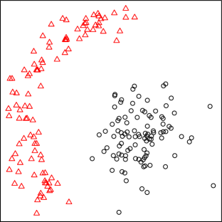
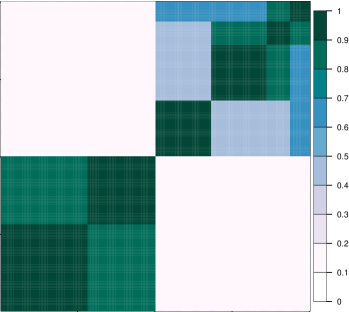
The Banana-clump dataset (Figure 2a) of Stuetzle & Nugent (2010) has 200 observations. FJ, DEMP+, GSL-NN and $K$-mH all reproduce the original partitioning but DEMP and the “elbow” approach of CM suggest three groups with the banana essentially halved. Figure 2b displays the heatmap obtained as part of $K$-mH. Two large clustered blocks are indicated with uncertainty over whether the upper right block should be partitioned further. (It is this partitioning that DEMP and CM go for.) Therefore, the heatmap displays the uncertainty and structure in the partitioning, but the $K$-mH algorithm chooses two groups.

(a) Bullseye Dataset

(b) Heatmap of Partitioning

Figure 3: (a) $K$-mH partitioning of the Banana-clump dataset and (b) heatmap illustrating clustering uncertainty and stability.

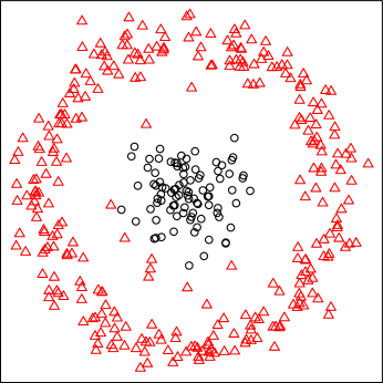
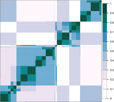
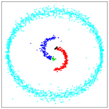
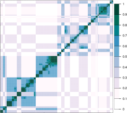
Revisiting the Bullseye dataset of Figure 1, we find that FJ, GSL-NN and $K$-mH produce good partitions (Figure 3a) with $\mathcal{R}\geq 0.99$ but DEMP, DEMP+ and CM perform poorly with the outer ring broken into several further groups. The heatmap (Figure 3b) indicates a lot of uncertainty but the methodology of Section 2.2.4 suggests two groups.

3.1.2 The Banana-spheres dataset:

This dataset has two separated banana-shaped half rings of 250 observations each that are surrounded by a third group in the shape of a full ring of 1500 observations. The observations in each group were simulated using pseudo-random realizations from different bivariate normal distributions with means that followed the central path of each shape. An additional 15 outlying observations from each cluster were added to provide a dataset of 3015 observations.

(a) $\mathcal{R}=0.99$, $K$ = 3

(b) $\mathcal{R}=0.95$, $K$ = 5

(c) $\mathcal{R}=0.74$, $K$ = 2

(d) $K$-mH heatmap

Figure 4: Top three partitionings of the Bananas-sphere dataset using (a) $K$-mH (b) FJ and (c) GSL-NN. Captions indicate estimated number of groups and $\mathcal{R}$ between estimated and true groupings. (d) $K$-mH heatmap for stability of groupings.

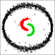
Figures 4a-c display the top three performers. $K$-mH chooses three groups with ${\mathcal{R}}=0.99$ while FJ chooses a 5-groups partition: however, the partitioning is still quite good ($\mathcal{R}=0.95$). GSL-NN suggests 2 clusters while the elbow plot of CM provides $K$ = 11 and ${\mathcal{R}}=0.53$. Both DEMP (${\mathcal{R}}=0.29$)and DEMP+ (${\mathcal{R}}=0.45$) do worse. Further the heatmap (Figure 4d) shows the structure in the dataset. While there are between 2 and 3 clear groups, there is also indication of the complicated structure of each group as well as the outliers.

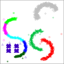
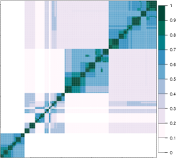
3.1.3 The SCX Dataset:

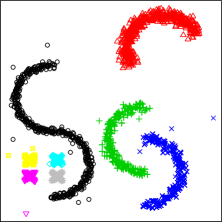
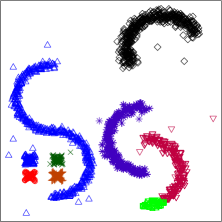
This dataset has a variety of cluster shapes and sizes, with three separated C-shaped groups rotated at different angles, a large S-shaped group and four small X-shaped groups. Twenty outlying observations are added to the clusters for a total of 3420 observations. Here, $K$-mH partitioning (Figure 5) is near-perfect (with two observations misclassified as scatter and not displayed in the dataset) while FJ is the next best performer. CM, DEMP and DEMP+ perform similarly, but GSL-NN finds 7 groups (${\mathcal{R}}=0.53$) clusters, with the S and 4 crosses all placed in one group and the two lower C’s split into 2 and three groups, respectively. The heatmap indicates uncertainty with 4 large groups with further definition and $K_{*}$ not easily identified. This uncertainty is reflected in the estimated $K_{*}$s which were 7, 8, 9, and 10, with frequency of occurrence 28, 48, 22, and 2% of the time, respectively. The median estimated $K_{*}=8$ yields the perfect solution of Figure 5a.

(a) $\mathcal{R}=0.99$, $K$ = 8

(b) $\mathcal{R}=0.89$, $K$ = 8

(c) $\mathcal{R}=0.78$, $K$ = 9

(d) $K$-mH heatmap

Figure 5: Top three performers for SCX: (a) $K$-mH (b) FJ and (c) CM and (d) the $K$-mH heatmap.

3.1.4 The Cigarette-Bullseye dataset

We have another

(a) $\mathcal{R}=1.0$, $K$ = 8

(b) $\mathcal{R}=0.99$, $K$ = 6

(c) $\mathcal{R}=0.96$, $K$ = 9

(d) $K$-mH heatmap

Figure 6: Top three performers on the Cigarette-Bullseye dataset: (a) $K$-mH, (b) CM, (c) FJ and (d) the $K$-mH heatmap.

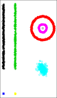
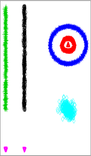
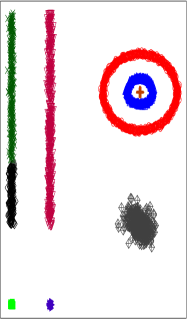
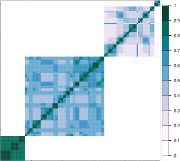
complex-structured dataset with 3 concentric ringed groups, 2 long groups above 2 small spherical ones and 1 group that is actually a superset of 2 overlapping Gaussian groups. $K$-mH and FJ perform similarly while CM finds 6 clusters but ${\mathcal{R}}=0.99$ because the smaller groups are the ones not identified clearly. GSL-NN also underestimates the number of groups to be 6, with ${\mathcal{R}}=0.78$. Both DEMP $({\mathcal{R}}=0.62)$ and DEMP+ $({\mathcal{R}}=0.64)$ exhibit poorer performance. The heatmap has similar characteristics as SCX, with 3-4 large groups but no clear choice for $K_{*}$ beyond that even though there are suggestions of sub-groups within each of the large groups. However, estimates of $K_{*}$ were 8 (50% of the time), 9 (42%) and 10 (8% of the time). The median $K_{*}=8$ yields the perfect $K$-mH solution of Figure 6a while $K_{*}=9$ breaks the leftmost long cluster further into two groups, yielding a similar partitioning as FJ (Figure 6c).

3.2 Higher-Dimensional Datasets

We next present performance evaluations on three higher-dimensional datasets often used in the literature.

3.2.1 Olive Oils:

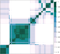
This dataset (Forina & Tiscornia, 1982; Forina et al., 1983) has measurements on 8 chemical components for 572 samples of olive oil taken from 9 different areas in Italy which are from three regions: Sardinia and Northern and Southern Italy. For this dataset, GSL-NN is the only method that identifies 9 groups (${\mathcal{R}}=0.61$) while FJ identifies 8 groups (${\mathcal{R}}=0.54$). CM (${\mathcal{R}}=0.75$), DEMP (${\mathcal{R}}=0.82$)and DEMP+ (${\mathcal{R}}=0.85$) are the best (${\mathcal{R}}=0.75$) performers even though they identify only 7 groups. The visualization step of the $K$-mH algorithm on the other hand largely identifies 8 kinds of olive oils (88% of the time) and also 7 (2%) and 9 (12%) kinds of olive oils. The median estimated $K_{*}=11$ yields a partitioning with ${\mathcal{R}}=0.67$. A closer look at the $K$-mH partitions reveals that oils from the southern areas of Calabria, Sicily and South Apulia are mainly grouped together in our second cluster while the remaining southern area of North-Apulia primarily populates our ninth cluster. Coastal and Inland Sardinian olive oils are identified very well by our groupings.

(a)

Region	Area	1	2	3	4	5	6	7	8	9	10	11
North	East Liguria	0	0	4	8	12	0	0	0	0	0	26
	Umbria	0	0	51	0	0	0	0	0	0	0	0
	West Liguria	0	0	0	0	37	0	0	0	0	13	0
Sardinia	Coastal Sardinia	0	0	0	0	0	0	3	30	0	0	0
	Inland Sardinia	0	0	0	0	0	0	65	0	0	0	0
South	Calabria	0	55	0	0	0	0	0	0	0	0	1
	North Apulia	0	1	0	0	0	0	0	0	24	0	0
	Sicily	5	17	0	0	0	8	0	0	6	0	0
	South Apulia	2	204	0	0	0	0	0	0	0	0	0

(b)

Figure 7: The $K$-mH heatmap and the results by region and area obtained from $K$-mH clustering of the Olive Oils dataset.

Our partitioning aligns very well with the three regions with our groups 3, 4, 5, 10 and 11 (with the exception of one oil) all exclusively from the north, groups 7 and 8 from Sardinia and groups 1, 2, 6 and 9 exclusively from the south. The near-perfect embedding of our groups within the three regions indicates that the nine areas drawn using political geography may not distinguish the different kinds of olive oils as well as a different characterization using a different set of sub-regions that are based on physical geography.

3.2.2 Zipcode Images:

The zipcode images dataset made available by Stuetzle & Nugent (2010) has been used in machine learning to evaluate clustering and classification algorithms and consists of 2000 $16\times 16$ images of handwritten Hindu-Arabic numerals. Thus, $p=256$ here. Stuetzle & Nugent (2010) report that GSL-NN “vaguely” finds 9 groups (${\mathcal{R}}=0.64$) but that their 10-groups solution is worse (${\mathcal{R}}=0.54$). We normalized the measurements for each digit to have zero mean and unit variance so that the Euclidean distance between any two observations is negatively but affinely related to the correlation between them. We reduced dimensions by principal components analysis and used the projection of the observations into the space spanned by the first 54 principal components which explain at least 90% of the variation in the data. This dataset is perhaps too cumbersome for CM, DEMP and DEMP+ while FJ finds 6 groups but the assignment is not very far from random (${\mathcal{R}}=0.05$).

(a)

		Zipcode Digit
Group		0	1	2	3	4	5	6	7	8	9
1		5	0	0	0	0	2	51	0	0	0
2		0	0	0	0	0	0	45	0	0	0
3		0	0	0	62	0	0	0	0	2	0
4		0	323	0	0	19	2	2	2	2	0
5		48	0	1	0	0	2	0	0	1	0
6		0	0	0	1	35	0	0	2	1	10
7		0	0	0	1	0	36	0	0	0	0
8		1	0	1	4	0	2	0	2	115	1
9		0	0	41	0	0	0	0	0	0	0
10		0	0	1	0	73	0	0	0	1	0
11		0	0	0	0	0	0	25	0	0	0
12		1	0	1	6	0	18	0	0	0	0
13		135	0	4	0	0	3	0	0	1	0
14		0	0	0	0	0	0	0	52	0	1
15		1	0	38	0	1	1	0	0	0	0
16		0	0	1	0	4	0	0	12	1	40
17		0	0	57	0	0	0	0	0	0	0
18		0	0	33	0	0	0	0	0	2	0
19		0	0	1	0	0	2	0	19	2	2
20		59	0	1	0	0	1	1	0	0	0
21		1	0	4	56	0	3	0	0	2	0
22		69	0	0	0	0	0	0	0	0	0
23		1	0	0	0	0	0	41	0	1	0
24		0	0	0	1	5	0	0	7	1	59
25		68	0	0	0	0	0	0	0	0	0
26		0	0	0	0	0	29	1	0	1	0
27		0	0	2	0	0	0	0	76	0	5
28		0	0	33	0	0	0	0	0	0	0
29		0	0	1	18	0	0	0	0	24	1
30		0	0	0	0	6	1	0	10	1	49

(b)

Figure 8: The $K$-mH heatmap and the results by digit obtained from $K$-mH clustering of the Zipcode dataset.

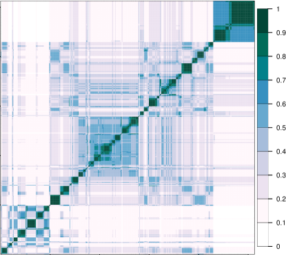
The $K$-mH heatmap (Figure 8) indicates lack of clarity in the number of groups with $K_{*}$ chosen at between 29 and 30 most of the time. The median $K_{*}=30$ yields the grouping (${\mathcal{R}}=0.54$) of Figure 8. Inspection indicates five main types of handwritten digits for 0 and 2, four kinds for 6, three kinds of 4 and 9, two major kinds of 3, 5 and 7 and one major kind for each of 1 and 8. Our groups correspond very reasonably to handwriting styles for digits and are very interpretable.

3.2.3 Handwritten Digits:

The Handwritten Digits dataset (Alimoglu, 1996; Alimoglu & Alpaydin, 1996) available from Newman et al. (1998) measured 16 attributes from 250 handwritten samples of 30 writers. With eight samples unavailable, this dataset has 10992 records. We used the first 7 principal component scores which explained 90% of the variation in the dataset. We were only able to apply FJ and $K$-mH (the other methods all threw up errors). FJ identified 10 groups

(a)

		Handwritten Digit
Group		0	1	2	3	4	5	6	7	8	9
1		2	359	1140	2	1	0	2	8	70	0
2		0	3	0	0	1	0	1050	0	0	0
3		0	0	0	0	0	0	0	79	48	0
4		17	2	0	1	1113	1	2	0	0	13
5		1	513	3	30	15	232	1	143	28	276
6		48	0	0	0	0	0	0	0	1	0
7		0	0	1	0	0	0	0	609	3	0
8		2	0	0	2	4	7	0	0	0	682
9		251	0	0	0	0	0	0	0	1	0
10		0	158	0	3	0	0	0	1	0	1
11		0	31	0	1017	0	13	0	0	5	5
12		228	0	0	0	0	0	0	0	0	0
13		0	0	0	0	0	3	0	0	408	1
14		1	0	0	0	0	0	0	0	488	0
15		57	0	0	0	0	0	0	0	0	0
16		0	1	0	0	0	0	0	302	1	0
17		0	0	0	0	0	1	0	0	0	38
18		1	0	0	0	0	0	0	0	0	24
19		0	0	0	0	10	174	0	0	0	15
20		416	0	0	0	0	0	0	0	0	0
21		0	0	0	0	0	624	1	0	2	0
22		0	76	0	0	0	0	0	0	0	0
23		100	0	0	0	0	0	0	0	0	0
24		19	0	0	0	0	0	0	0	0	0

(b)

Figure 9: The $K$-mH heatmap and the results by digit obtained from $K$-mH clustering of the Handwritten Digits dataset.

but performs very poorly (${\mathcal{R}}=0.097$) while the $K$-mH heatmap (Figure 9) identifies a range of $K_{*}=19$ through 27, with a median of 24. The $K$-mH grouping for $K_{*}=24$ yielded moderately good performance (${\mathcal{R}}=0.64$). Interestingly, our groups identified 2, 4 and 6 well, but not with a simpler digit like 1, which, in the light of our findings in Section 3.2.2, may suggest that the 16 attributes used to characterize the samples may have focused more on some features of the handwriting of digits.

Table 1: Performance in terms of $\mathcal{R}$ (first row of each block) and estimated number of groups $\hat{K}$ (second row of each block) for all datasets used in the experiment. A “-” indicates that the algorithm failed to converge or returned an error message.

Dataset		Measure	Method
Name	$(N,p,K)$		FJ	CM	GSL-NN	DEMP	DEMP+	$K$-mH
Banana-Clump	(200,2,2)	${\mathcal{R}}$	1.0	0.78	1.0	0.77	1.0	1.0
		$\hat{K}$	2	3	2	3	2	2
Bullseye	(400,2,2)	${\mathcal{R}}$	0.99	0.53	0.74	0.21	0.31	0.99
		$\hat{K}$	2	5	2	7	6	2
Banana-Spheres	(3015,2,3)	${\mathcal{R}}$	0.95	0.53	0.74	0.29	0.45	0.99
		$\hat{K}$	5	11	2	18	13	3
SCX	(3420,2,8)	${\mathcal{R}}$	0.89	0.78	0.53	0.77	0.78	1.0
		$\hat{K}$	8	12	7	12	12	8
Cigarette-Bullseye	(3025,2,8)	${\mathcal{R}}$	0.96	0.99	0.78	0.62	0.64	1.0
		$\hat{K}$	9	6	6	11	10	8
Olive Oils	(572,8,9)	${\mathcal{R}}$	0.54	0.75	0.61	0.82	0.85	0.67
		$\hat{K}$	8	7	9	7	7	11
Zipcode Digits	(2000,256,10)	${\mathcal{R}}$	0.05	-	0.64	-	-	0.54
		$\hat{K}$	8	-	9	-	-	26
Handwritten Digits	(10992,16,10)	${\mathcal{R}}$	0.10	-	-	-	-	0.64
		$\hat{K}$	10	-	-	-	-	24
Number of cases where a competitor performs better			6	8	7	8	6	2

The performances of $K$-mH, FJ, CM, DEMP and DEMP+ for all cases are summarized in Table 1 and shows that $K$-mH is always among the top performers. This happens with very complicated as well as simpler structures. Even when performance is not outstanding, as happened with higher-dimensional real-life datasets, $K$-mH is still a top performer, often producing results that are interpretable. FJ is also a good performer in the two-dimensional examples but this performance degraded more in higher dimensions than with $K$-mH. DEMP ad DEMP+ was a good performer only on the Olive Oils dataset where it performed very well despite underestimating the number of groups by 2. Our algorithm was also able to handle computations for the larger handwritten digits dataset.

4 Discussion

In this paper we propose a new $K$-means hierarchical clustering algorithm that builds on the idea of Fred & Jain (2005) that different clusterings of a dataset each provide different discrete evidence of a grouping. We compare several different clusterings of the data and choose the final grouping that is most similar to the proposed partitions. Our algorithm is among the top performing methods for both simulated datasets with complicated shapes as well as several real datasets. We also present an automated clustering approach for finding the optimal parition and number of groups that is shown to perform well. In addition, we use a graphical method introduced in Fred & Jain (2005) that we use to investigate uncertainty and structural stability of the clustering and to determine the correct number of groups. Our $K$-mH algorithm is computationally efficient for larger datasets in comparison to several other cluster merging algorithms. Indeed, the main computational cost is that of performing $K$-means for different $K$, which can be expensive given the number of initializing runs for each $K$. Further, it is very easily coded: simple R functions doing the same are available on request.

There are several directions for future work. One possibility is to compare other distance measures in the hierarchical step of the $K$-mH algorithm. It may be worthwhile to further use other different distance measures as candidate partitions when choosing the optimal partition $P_{*}$. Another aspect worthy of investigation would be to explore additional ways for determining $K_{*}$. It is worth noting in this context that the hierarchical map for visualizing structural stability can be a memory-intensive operation. Thus, we see that while we have put forward a promising algorithm, issues meriting further attention remain.

This research was supported, in part, by National Science Foundation (NSF) grants DMS-0707069, DMS-CAREER-0437555 and by the National Institutes of Health grant R21EB0126212. The content of this paper however is solely the responsibility of the authors and does not represent the official views of the NSF or the NIH.

References

- Alimoglu (1996) Alimoglu, F (1996), Combining Multiple Classifiers for Pen-Based Handwritten Digit Recognition, Master’s thesis, Institute of Graduate Studies in Science and Engineering, Bogazici University.
- Alimoglu & Alpaydin (1996) Alimoglu, F & Alpaydin, E (1996), ‘Methods of combining multiple classifiers based on different representations for pen-based handwriting recognition,’ in Proceedings of the Fifth Turkish Artificial Intelligence and Artificial Neural Networks Symposium (TAINN 96), Istanbul, Turkey.
- Baudry et al. (2010) Baudry, JP, Raftery, AE, Celeux, G, Lo, K & Gottardo, R (2010), ‘Combining mixture components for clustering.’ Journal of Computational and Graphical Statistics, 19(2), pp. 332–353.
- Byers & Raftery (1998) Byers, S & Raftery, AE (1998), ‘Nearest neighbor clutter removal for estimating features in spatial point processes,’ Journal of the American Statistical Association, 93, pp. 577–584.
- Everitt et al. (2001) Everitt, BS, Landau, S & Leesem, M (2001), Cluster Analysis (4th ed.), Hodder Arnold, New York.
- Forina et al. (1983) Forina, M, Armanino, C, Lanteri, S & Tiscornia, E (1983), ‘Classification of olive oils from their fatty acid composition,’ in Food Research and Data Analysis, Applied Science Publishers, London, p. 189 214.
- Forina & Tiscornia (1982) Forina, M & Tiscornia, E (1982), ‘Pattern recognition methods in the prediction of italian olive oil origin by their fatty acid content,’ Annali di Chimica, 72, p. 143 155.
- Fraley & Raftery (2002) Fraley, C & Raftery, AE (2002), ‘Model-based clustering, discriminant analysis, and density estimation,’ Journal of the American Statistical Association, 97, pp. 611–631.
- Fred & Jain (2005) Fred, AL & Jain, AK (2005), ‘Combining multiple clusterings using evidence accumulation,’ IEEE Transactions on Pattern Analysis and machine Intelligence, 27(6), pp. 835–850.
- Hartigan (1985) Hartigan, JA (1985), ‘Statistical theory in clustering,’ Journal of Classification, 2, pp. 63–76.
- Hartigan & Wong (1979) Hartigan, JA & Wong, MA (1979), ‘A -means clustering algorithm,’ Applied Statistics, 28, pp. 100–108.
- Hennig (2010) Hennig, C (2010), ‘Methods for merging Gaussian mixture components,’ Advances in Data Analysis and Classification, 4(1), pp. 3–34, 10.1007/s11634-010-0058-3.
- Hubert & Arabie (1985) Hubert, L & Arabie, P (1985), ‘Comparing partitions,’ Journal of Classification, 2, pp. 193–218.
- Johnson & Wichern (2007) Johnson, RA & Wichern, DW (2007), Applied Multivate Statical Analysis, Prentice-Hall, 6 edn.
- Kaufman & Rousseuw (1990) Kaufman, L & Rousseuw, PJ (1990), Finding Groups in Data, John Wiley and Sons, Inc., New York.
- Kettenring (2006) Kettenring, JR (2006), ‘The practice of cluster analysis,’ Journal of classification, 23, pp. 3–30.
- Krzanowski & Lai (1988) Krzanowski, WJ & Lai, YT (1988), ‘A criterion for determining the number of groups in a data set using sum-of-squares clustering,’ Biometrics, 44, pp. 23–34.
- MacQueen (1967) MacQueen, J (1967), ‘Some methods of classification and analysis of multivariate observations,’ Proceedings of the Fifth Berkeley Symposium on Mathematical Statistics and Probability, pp. 281–297.
- Maitra (2009) Maitra, R (2009), ‘Initializing partition-optimization algorithms,’ IEEE/ACM Transactions on Computational Biology and Bioinformatics, 6, pp. 144–157, http://doi.ieeecomputersociety.org/10.1109/TCBB.2007.70244.
- Maitra et al. (2012) Maitra, R, Melnykov, V & Lahiri, S (2012), ‘Bootstrapping for significance of compact clusters in multi-dimensional datasets,’ Journal of the American Statistical Association, 107(497), pp. 378–392, http://dx.doi.org/10.1080/01621459.2011.646935.
- Maitra & Ramler (2009) Maitra, R & Ramler, IP (2009), ‘Clustering in the presence of scatter,’ Biometrics, 65, pp. 341–352.
- Marriott (1971) Marriott, FH (1971), ‘Practical problems in a method of cluster analysis,’ Biometrics, 27, pp. 501–514.
- McLachlan (1987) McLachlan, G (1987), ‘On bootstrapping the likelihood ratio test statistic for the number of components in a normal mixture,’ Applied Statistics, 36, pp. 318–324.
- McLachlan & Peel (2000) McLachlan, G & Peel, D (2000), Finite Mixture Models, John Wiley and Sons, Inc., New York.
- McLachlan & Basford (1988) McLachlan, GJ & Basford, KE (1988), Mixture Models: Inference and Applications to Clustering, Marcel Dekker, New York.
- Melnykov (2016) Melnykov, V (2016), ‘Merging mixture components for clustering through pairwise overlap,’ Journal of Computational and Graphical Statistics, 25(1), pp. 66–90.
- Melnykov & Maitra (2011) Melnykov, V & Maitra, R (2011), ‘CARP: Software for fishing out good clustering algorithms,’ Journal of Machine Learning Research, 12, pp. 69 – 73.
- Muirhead (2005) Muirhead, R (2005), Aspects of Multivariate Statistical Theory, Wiley, 2 edn.
- Murtagh (1985) Murtagh, F (1985), Multi-dimensional clustering algorithms, Springer-Verlag, Berlin; New York.
- Newman et al. (1998) Newman, D, Hettich, S, Blake, CL & Merz, CJ (1998), ‘UCI repository of machine learning databases,’ .
- R Core Team (2017) R Core Team (2017), R: A Language and Environment for Statistical Computing, R Foundation for Statistical Computing, Vienna, Austria.
- Ramey (1985) Ramey, DB (1985), ‘Nonparametric clustering techniques,’ in Encyclopedia of Statistical Science, Wiley, New York, vol. 6, pp. 318–319.
- Stuetzle & Nugent (2010) Stuetzle, W & Nugent, R (2010), ‘A generalized single linkage method for estimating the cluster tree of a density,’ JCGS, 19(2), pp. 397–418.
- Sugar & James (2003) Sugar, CA & James, GM (2003), ‘Finding the number of clusters in a dataset,’ Journal of the American Statistical Association, 98(463).
- Tibshirani et al. (2003) Tibshirani, RJ, Walther, G & Hastie, TJ (2003), ‘Estimating the number of clusters in a dataset via the gap statistic,’ Journal of the Royal Statistical Society, 63(2), pp. 411–423.
- Tseng & Wong (2005) Tseng, GC & Wong, WH (2005), ‘Tight clustering: A resampling-based approach for identifying stable and tight patterns in data,’ Biometrics, 61, pp. 10–16.