Stochastic Geometry Modeling and Analysis of Single- and Multi-Cluster Wireless Networks

Seyed Mohammad Azimi-Abarghouyi, Behrooz Makki,
 Martin Haenggi, , Masoumeh Nasiri-Kenari, , and Tommy Svensson
S.M. Azimi-Abarghouyi and M. Nasiri-Kenari are with the Dep. of Electrical Engineering, Sharif University of Technology, Tehran 11365-9363, Iran. (e-mail: azimi__\_sm@ee.sharif.edu; mnasiri@sharif.edu). B. Makki and T. Svensson are with the Dep. of Signals and Systems, Chalmers University of Technology, 412 96 Gothenburg, Sweden. (e-mail: {{\{behrooz.makki, tommy.svensson}}\}@chalmers.se). M. Haenggi is with the Dept. of Electrical Engineering, University of Notre Dame, IN 46556, USA. (e-mail: mhaenggi@nd.edu). This work has been supported in part by the Research Office of Sharif University of Technology under grant QB960605 and by the VR Research Link Project "Green Communications" and by the U.S. National Science Foundation under grant CCF 1525904.
Abstract

This paper develops a stochastic geometry-based approach for the modeling and analysis of single- and multi-cluster wireless networks. We first define finite homogeneous Poisson point processes to model the number and locations of the transmitters in a confined region as a single-cluster wireless network. We study the coverage probability for a reference receiver for two strategies; closest-selection, where the receiver is served by the closest transmitter among all transmitters, and uniform-selection, where the serving transmitter is selected randomly with uniform distribution. Second, using Matern cluster processes, we extend our model and analysis to multi-cluster wireless networks. Here, the receivers are modeled in two types, namely, closed- and open-access. Closed-access receivers are distributed around the cluster centers of the transmitters according to a symmetric normal distribution and can be served only by the transmitters of their corresponding clusters. Open-access receivers, on the other hand, are placed independently of the transmitters and can be served by all transmitters. In all cases, the link distance distribution and the Laplace transform (LT) of the interference are derived. We also derive closed-form lower bounds on the LT of the interference for single-cluster wireless networks. The impact of different parameters on the performance is also investigated.

Index Terms:
Stochastic geometry, coverage probability, clustered wireless networks, Poisson point process, Matern cluster process.

I Introduction

Single-cluster wireless networks are composed of a number of nodes distributed inside a finite region. This spatial setup is an appropriate model for, e.g., various millimeter wave communications use-case scenarios, indoor and ad hoc networks, as promising candidate technologies for the next generation of wireless networks [1]-[2]. This setup is also useful in situations where there is a range limit for backhaul links in connecting transmitters to a core network, e.g., cloud radio access networks [3]. On the other hand, the ever-growing randomness and irregularity in the locations of nodes in a wireless network has led to a growing interest in the use of stochastic geometry and Poisson point processes (PPPs) for accurate, flexible, and tractable spatial modeling and analysis [4]-[9].

In comparison to wireless networks on infinite regions that are mostly modeled by the infinite homogeneous PPP (HPPP) [10, Def. 2.8], the modeling and performance analysis of single-cluster wireless networks is more challenging and requires different approaches. The main challenge is that a finite point process is not statistically similar from different locations, and therefore, the system performance depends on the receiver location even after averaging over the point process.

The stochastic geometry-based modeling and analysis of single-cluster wireless networks modeled as a binomial point process (BPP) [10, Def. 2.11] has been well studied [11]-[21]. In the BPP model, a fixed and finite number of nodes are distributed independently and uniformly inside a finite region. Most prior works focus on a setup where the reference receiver is placed at the center of a circular network region [11]-[15]. Also, considering a circular region, [16] has recently developed a comprehensive framework for performance characterizations of an arbitrarily-located reference receiver inside the region under different transmitter selection strategies. Considering transmitters at a non-zero fixed altitude, disk-shaped networks of unmanned aerial vehicles are analyzed in [17]. There are also a few studies that present outage probability characterizations of a fixed link inside an arbitrarily-shaped finite region [18]-[21].

In spite of the usefulness of HPPP for modeling and analysis of coverage-centric and uniform deployments of nodes [4]-[10], it cannot accurately model user-centric and content-centric deployments, where the nodes may be deployed at the places with high user density [22]-[24]. In such deployments, it is important to take into account non-uniformity as well as the correlation that may exist between the locations of the transmitters and receivers. Accordingly, third generation partnership project (3GPP) has considered clustered models in [24]-[25]. Models based on Poisson cluster processes (PCPs) [10, Sec. 3.4] have recently been studied for heterogeneous [22] and device-to-device (D2D) networks [23]. In these works, the network follows a Thomas cluster process (TCP) [10, Def. 3.5]. A PCP model is also proposed and analyzed for heterogeneous networks in [26]. In [27], clustered ad hoc networks are modeled using the Matern cluster process (MCP) [10, Def. 3.6] and the TCP, and the performance of a fixed link is analyzed. Nearest-neighbor and contact distance distributions for the MCP are derived in [28].

In this paper, we develop tractable models for single- and multi-cluster wireless networks. We define a finite homogeneous Poisson point process (FHPPP) to model nodes in a finite region and then develop a framework for the analysis of single-cluster wireless networks under two different strategies. The first approach is referred to as closest-selection where a reference receiver is served by the closest transmitter in the network. In the second approach, which we refer to as uniform-selection, a uniformly randomly selected transmitter is connected to the receiver. These strategies cover a broad range of requirements of wireless networks. For instance, the closest-selection approach is suitable for cellular networks, while the uniform-selection scheme is relevant to ad hoc networks.

To model multi-cluster wireless networks consisting of different single-cluster wireless networks, we consider an MCP of transmitters. For the receivers, we consider two types, i) closed-access receivers, which are located around the cluster centers of transmitters with a symmetric normal distribution and are allowed to be served only by the transmitters of their corresponding clusters according to the closest- or uniform-selection strategy, and ii) open-access receivers, which can be served by all transmitters according to the closest-selection strategy.

We derive exact expressions for the coverage probability of a reference receiver in single- and multi-cluster wireless networks for the different selection strategies and types of receivers. For each selection strategy and type of receiver in single- and multi-cluster wireless networks, we characterize the Laplace transform (LT) of the interference. Moreover, as a key step for the coverage probability analysis, the distributions of the distance from the reference receiver to its serving transmitter are derived. We also derive tight closed-form lower bounds on the LT of the interference in the case of single-cluster wireless networks, which are convenient for the coverage probability analysis.

We investigate the impact of different parameters of the system models on the performance in terms of the coverage probability and spectral efficiency. In most cases, a higher path loss exponent improves the performance. However, at relatively high distances of the reference receiver to the center of single-cluster wireless networks, a higher path loss has a degrading effect on the performance. Also, an increase in the distance of the reference receiver to the center of the network decreases the chance for coverage. Our analysis reveals that there exists an optimal distance for the location of the reference receiver from the center of the network that maximizes the coverage probability. An optimal distance is also observed for the spectral efficiency. Our evaluation also shows that, for a broad range of parameter settings, our proposed lower bounds tightly mimic the exact results on the coverage probability.

Our work is different from the state-of-the-art literature, e.g., [10]-[23], [26]-[28], from three perspectives. First, different from the BPP, which models a fixed number of nodes in a region, we consider a point process that is suitable for finite regions with a random number of nodes and allow for arbitrary receiver locations. Second, we comprehensively study multi-cluster wireless networks using the MCP. In our analysis, we also derive the contact distribution function of the MCP in a form that is significantly simpler than the one in [28, Thm. 1]. Third, we propose open-access and closed-access receivers and different transmitter selection strategies.

The rest of the paper is organized as follows. Section II describes the system models. Secion III proposes the transmitter selection strategies and presents the analytical results for the coverage probability of single-cluster wireless networks, including characterizations for the serving distance distributions, and the LT of the interference and its corresponding lower bounds. Section IV presents the analytical results for the coverage probability of multi-cluster wireless networks, and derives the related serving distance distributions and the LT of the interferences. Section V presents the numerical results. Finally, Section VI concludes the paper.

II System Model

In this section, we provide a mathematical model of the system, including the spatial distribution of the nodes for single- and multi-cluster wireless networks and the channel model.

II-A Spatial Model for Single-Cluster Wireless Networks

Let us define an FHPPP as follows.

Definition 1

We define the FHPPP as Φ=𝒫𝒜Φ𝒫𝒜{\Phi}=\mathcal{P}\cap{\cal A}, where 𝒫𝒫\mathcal{P} is an HPPP of intensity λ𝜆\lambda and 𝒜2𝒜superscript2{\cal A}\subset\mathbb{R}^{2}.                                                                                                                              ∎

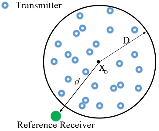
We consider a single-cluster wireless network as shown in Fig. 1, where the locations of active transmitters are modeled as an FHPPP. The transmitters are assumed to transmit at the same power. For simplicity and in harmony with, e.g., [11]-[17], we let 𝒜=𝐛(𝐱𝐨,D)𝒜𝐛subscript𝐱𝐨𝐷{\mathbf{\cal A}}=\mathbf{b}(\mathbf{x}_{\mathbf{o}},D), where 𝐛(𝐱𝐨,D)𝐛subscript𝐱𝐨𝐷\mathbf{b}(\mathbf{x}_{\mathbf{o}},D) represents a disk centered at 𝐱𝐨subscript𝐱𝐨\mathbf{x}_{\mathbf{o}} with radius D𝐷D. However, our theoretical results can be extended to arbitrary regions 𝒜𝒜\cal A.

Receivers can be located everywhere in 2superscript2\mathbb{R}^{2}. With no loss of generality, we conduct the analysis at a reference receiver located at the origin 𝐨𝐨\mathbf{o}. We further define d=𝐱𝐨𝑑normsubscript𝐱𝐨d=\|\mathbf{x}_{\mathbf{o}}\|.

The proposed setup well models a wireless network confined in a finite region, such as indoor and ad hoc networks.
Refer to caption
Figure 1: An illustration of the system model for single-cluster wireless networks.

II-B Spatial Model for Multi-Cluster Wireless Networks

An MCP is defined as follows [10, Def. 3.6].

Definition 2

An MCP ΦΦ{\Phi} is a union of offspring points that are located around parent points. The parent point process is an HPPP ΦpsubscriptΦp{\Phi}_{\rm p} with intensity λpsubscript𝜆p\lambda_{\rm p}, and the offspring point processes (one per parent) are conditionally independent. Conditioned on 𝐱Φp𝐱subscriptΦp\mathbf{x}\in{\Phi}_{\rm p}, the offsprings form an FHPPP Φ𝐱subscriptΦ𝐱{\Phi}_{\mathbf{x}} with intensity λ𝜆\lambda over the disk 𝐛(𝐱,D)𝐛𝐱𝐷\mathbf{b}(\mathbf{x},D).                                                                           ∎

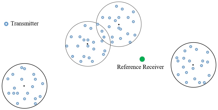
We consider a multi-cluster wireless network as shown in Fig. 2, where the locations of active transmitters are modeled as an MCP.

We consider two types of receivers. The first type, referred to as closed-access receivers, can be served by only a single cluster of transmitters. This closed-access receiver is distributed according to a symmetric normal distribution with variance σc2superscriptsubscript𝜎c2\sigma_{\text{c}}^{2} around the parent point of its corresponding cluster. Therefore, assuming a closed-access receiver at 𝐲𝐲\mathbf{y} and its parent point at 𝐱𝐱\mathbf{x}, 𝐱𝐲norm𝐱𝐲\|\mathbf{x}-\mathbf{y}\| is Rayleigh distributed with probability density function (PDF)

f𝐱𝐲(v)=vσc2exp(v22σc2).subscript𝑓norm𝐱𝐲𝑣𝑣superscriptsubscript𝜎c2superscript𝑣22superscriptsubscript𝜎c2\displaystyle{f_{\|\mathbf{x}-\mathbf{y}\|}}\left(v\right)=\frac{v}{{{\sigma_{\text{c}}^{2}}}}{\rm{\exp}}\left({-\frac{{{{v}^{2}}}}{{2{\sigma_{\text{c}}^{2}}}}}\right). (1)

The second type, referred to as open-access receivers, considers receivers that are placed independently of the transmitters and can be served by all transmitters.
Refer to caption
Figure 2: An illustration of the system model for a finite piece of multi-cluster wireless networks.

The proposed setup well models various use-case scenarios as follows:

1) Clustered Small-Cell Base Stations (BSs): The trend in cellular networks is to deploy small-cell BSs at the places with high user density, referred to as user-centric networks [22], [29], as also proposed in 3GPP [24]-[25]. In this way, according to our setup, users who are likely to be close to a cluster of small-cell BSs can be modeled as closed-access receivers, such as users at a stadium or a mall. The open-access receivers can model users who are distributed homogeneously and independently of the small-cell BS locations, such as pedestrians or cars.

2) Cloud BSs: A cloud BS is a distributed multiple-antenna system formed by a number of simple antenna terminals [30]. In this application, the closed-access receivers can be modeled as the users who have a license to use a certain BS, while the open-access receivers can model users with flexibility to access all BSs.

3) Clustered Access Networks: A large building may have a number of WiFi access points as an access network to meet its users’ demands. The closed-access receivers model the users who are in a building and use its access network. On the other hand, the open-access receivers are users who can handoff between access networks of different buildings.

4) Clustered D2D Networks: A device typically has nearby devices in a finite region as a cluster in a content-centric network, which can have direct communications with each other. The closest- or uniform-selection strategy can be considered for cellular or ad hoc access to contents distributed over the devices, respectively.

II-C Channel Model

We assume distance-dependent power-law path loss and small-scale Rayleigh fading. Thus, the received power at the reference receiver from a transmitter located at 𝐲𝐲\mathbf{y} is h𝐲𝐲αsubscript𝐲superscriptnorm𝐲𝛼{h_{\mathbf{y}}}{\|\mathbf{y}\|^{-\alpha}}, where the (common) transmit power is set to 1 with no loss of generality and α>2𝛼2\alpha>2 is the path loss exponent. The sequence {h𝐲}subscript𝐲\left\{h_{\mathbf{y}}\right\} consists of i.i.d. exponential random variables with mean 1.

III Single-Cluster Wireless Networks

In this section, we concentrate on single-cluster wireless networks. To allocate a transmitter to a reference receiver, we propose selection strategies in Subsection III.A. Then, distance distributions and coverage probabilities for the selection strategies are derived in Subsections III.B and III.C, respectively. However, the resulting expressions for the coverage probabilities are not very easy to use. Hence, we derive a closed-form lower bound for the coverage probability of each strategy in Subsection III.D.

III-A Selection Strategies

1) Closest-selection. Here, a reference receiver is served by the transmitter that provides the maximum received power averaged over the fading. In our model, this leads to the closest-selection strategy, i.e.,

𝐱c=argmin𝐲{Φn(Φ)>0}𝐲,subscript𝐱csubscript𝐲conditional-setΦ𝑛Φ0norm𝐲\displaystyle{{\rm{\mathbf{x}}_{\text{c}}}}=\arg\mathop{\min}\limits_{{\mathbf{y}}\in\left\{{\Phi}\mid n({\Phi})>0\right\}}\|{{\mathbf{y}}}\|, (2)

where n()𝑛n(\cdot) denotes the number of elements in a set. Suitable for networks with infrastructure such as downlink cellular networks, this strategy implies that a receiver is served by the transmitter whose Voronoi cell it resides in [4]-[23].

2) Uniform-selection. Here, the serving transmitter is selected randomly with uniform distribution among all transmitters. This leads to

𝐱u=Unif{Φn(Φ)>0},subscript𝐱uUnifconditional-setΦ𝑛Φ0\displaystyle{{\rm{\mathbf{x}}_{\text{u}}}}=\text{Unif}\left\{{\Phi}\mid n(\Phi)>0\right\}, (3)

where Unif{}Unif\text{Unif}\left\{\cdot\right\} denotes the uniform-selection operation. Uniform-selection models random allocation of receivers to transmitters, which may be the case in networks without infrastructure, e.g., ad hoc networks and D2D networks [16], [23]. It is also suitable for applications where the content of interest for a receiver can be available at each transmitter among all transmitters with equal probability, such as caching networks.

The signal-to-interference-and-noise ratio (SINR) of a reference receiver at the origin can be expressed as

SINRq=h𝐱q𝐱qασ2+q,q={c,u},formulae-sequencesubscriptSINR𝑞subscriptsubscript𝐱𝑞superscriptnormsubscript𝐱𝑞𝛼superscript𝜎2subscript𝑞𝑞cu\displaystyle\text{SINR}_{q}=\frac{{{h_{\mathbf{x}_{q}}}{{{\|\mathbf{x}_{q}\|}^{-\alpha}}}}}{{{\sigma^{2}}+{\cal I}_{q}}},\ q=\left\{\text{c},\text{u}\right\}, (4)

where 𝐱qsubscript𝐱𝑞\mathbf{x}_{q} is the location of the serving transmitter, q=𝐲Φ\{𝐱q}h𝐲𝐲αsubscript𝑞subscript𝐲\Φsubscript𝐱𝑞subscript𝐲superscriptnorm𝐲𝛼{\cal I}_{q}=\mathop{\sum}\nolimits_{\mathbf{y}\in{\Phi}\backslash\left\{\mathbf{x}_{q}\right\}}{h_{\mathbf{y}}}{\|\mathbf{y}\|^{-\alpha}} denotes the interference, and σ2superscript𝜎2\sigma^{2} is the noise power. To distinguish between the strategies, q=c𝑞cq=\text{c} and u represent the case of closest- and uniform-selection strategies, respectively. For notational simplicity, let us also define Rq=𝐱qsubscript𝑅𝑞normsubscript𝐱𝑞R_{q}=\|\mathbf{x}_{q}\|.

III-B Serving Distance Distribution

Considering the closest- and uniform-selection strategies, in this subsection, we derive the distributions of the distance from the reference receiver to its serving transmitter. These distance distributions will be used later in the coverage probability analysis.

Let us first define φ0=sin1(Dd)subscript𝜑0superscript1𝐷𝑑\varphi_{0}={\sin^{-1}}\left({\frac{D}{d}}\right), φ1(r)=cos1(r2+d2D22dr)subscript𝜑1𝑟superscript1superscript𝑟2superscript𝑑2superscript𝐷22𝑑𝑟\varphi_{1}(r)={\cos^{-1}}\left({\frac{{{r^{2}}+{d^{2}}-{D^{2}}}}{{2dr}}}\right), R1(θ)=dcos(θ)+D2d2sin2(θ)subscript𝑅1𝜃𝑑𝜃superscript𝐷2superscript𝑑2superscript2𝜃R_{1}(\theta)=d\cos\left(\theta\right)+\\ \sqrt{{D^{2}}-{d^{2}}{{\sin}^{2}}\left(\theta\right)} and R^1(θ)=dcos(θ)D2d2sin2(θ)subscript^𝑅1𝜃𝑑𝜃superscript𝐷2superscript𝑑2superscript2𝜃\hat{R}_{1}(\theta)=d\cos\left(\theta\right)-\sqrt{D^{2}-{d^{2}}{{\sin}^{2}}\left(\theta\right)}, and present a lemma on the intersection area of two circles.

Lemma 1

Consider two circles with radii D𝐷D and r𝑟r with centers separated by distance d𝑑d. The area of their intersection is given by [31, Eq. (12.76)]

d(r)=D2cos1(D2+d2r22dD)+r2φ1(r)12[(r+d)2D2][D2(rd)2].subscript𝑑𝑟superscript𝐷2superscript1superscript𝐷2superscript𝑑2superscript𝑟22𝑑𝐷superscript𝑟2subscript𝜑1𝑟12delimited-[]superscript𝑟𝑑2superscript𝐷2delimited-[]superscript𝐷2superscript𝑟𝑑2\displaystyle{{\cal B}_{d}}(r)=D^{2}{\cos^{-1}}\left({\frac{{D^{2}+{d^{2}}-r^{2}}}{{2d{D}}}}\right)+r^{2}\varphi_{1}(r)-\frac{1}{2}\sqrt{\left[{{{\left({{r}+d}\right)}^{2}}-D^{2}}\right]\left[{D^{2}-{{\left({{r}-d}\right)}^{2}}}\right]}. (5)

Considering the closest-selection strategy, the distance from the reference receiver to its nearest transmitter Rcsubscript𝑅cR_{\text{c}} is larger than r𝑟r if and only if at least one transmitter exists inside 𝒜𝒜\cal A and there is no transmitter located within 𝐛(𝐨,r)𝒜𝐛𝐨𝑟𝒜\mathbf{b}(\mathbf{o},r)\cap\cal A. Letting 𝒞rsubscript𝒞𝑟{\rm{\cal C}}_{r} denote the intersection, we have

(Rc>r)=(n(Φ𝒞r)=0 and n(Φ)>0)(n(Φ)>0)subscript𝑅c𝑟𝑛Φsubscript𝒞𝑟0 and 𝑛Φ0𝑛Φ0\displaystyle{\mathbb{P}}\left({R_{\text{c}}>r}\right)=\frac{\mathbb{P}(n(\Phi\cap{\cal C}_{r})=0\text{ and }n(\Phi)>0)}{\mathbb{P}(n({\Phi})>0)}\hskip 190.0pt
=(a)(n(Φ𝒞r)=0)(n(Φ𝒞r)>0)(n(Φ)>0)superscript𝑎absent𝑛Φsubscript𝒞𝑟0𝑛Φsubscript𝒞𝑟0𝑛Φ0\displaystyle\stackrel{{\scriptstyle(a)}}{{=}}\frac{\mathbb{P}(n(\Phi\cap{\cal C}_{r})=0)\mathbb{P}(n(\Phi\setminus{\cal C}_{r})>0)}{\mathbb{P}(n({\Phi})>0)}\hskip 177.0pt
=(b)exp(λ|𝒞r|)(1exp(λ(πD2|𝒞r|)))1exp(λπD2)=exp(λ|𝒞r|)exp(λπD2)1exp(λπD2),superscript𝑏absent𝜆subscript𝒞𝑟1𝜆𝜋superscript𝐷2subscript𝒞𝑟1𝜆𝜋superscript𝐷2𝜆subscript𝒞𝑟𝜆𝜋superscript𝐷21𝜆𝜋superscript𝐷2\displaystyle\stackrel{{\scriptstyle(b)}}{{=}}\frac{\exp\left({-{\rm{\lambda}}\left|{\rm{\cal C}}_{r}\right|}\right)(1-\exp({-{\rm{\lambda}}(\pi D^{2}-\left|{\rm{\cal C}}_{r}\right|})))}{1-\exp(-\lambda\pi D^{2})}=\frac{\exp\left({-{\rm{\lambda}}\left|{\rm{\cal C}}_{r}\right|}\right)-\exp({-\lambda\pi D^{2}})}{1-\exp(-\lambda\pi D^{2})}, (6)

where |||\cdot| denotes the area of a region. Also, (a)𝑎(a) follows from the fact that the numbers of points of a PPP in disjoint regions are independent, and (b)𝑏(b) is because RcD+dsubscript𝑅c𝐷𝑑R_{\text{c}}\leq D+d. Note when the intersection is the whole of 𝒜𝒜\cal A, i.e., |𝒞r|=πD2subscript𝒞𝑟𝜋superscript𝐷2|{\cal C}_{r}|=\pi D^{2}, (6) is zero.

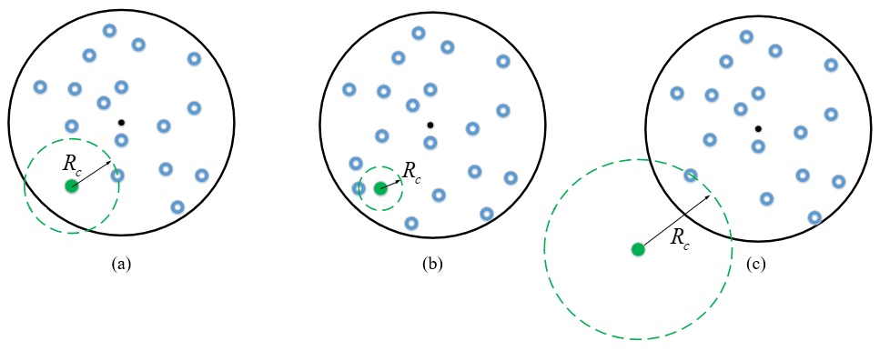
According to Fig. 3, which shows illustrations of the intersection, there are two different cases as follows.
Refer to caption
Figure 3: An illustration of the intersection in the case dD𝑑𝐷d\leq D for Subplot (a): DdRc<D+d𝐷𝑑subscript𝑅c𝐷𝑑D-d\leq R_{\text{c}}<D+d and Subplot (b): 0Rc<Dd0subscript𝑅c𝐷𝑑0\leq R_{\text{c}}<D-d, and in the case d>D𝑑𝐷d>D for Subplot (c): dDRc<d+D𝑑𝐷subscript𝑅c𝑑𝐷d-D\leq R_{\text{c}}<d+D.

Case 1: If dD𝑑𝐷d\leq D, then

|𝒞r|={πr20r<Dd,d(r)Ddr<D+d,πD2rD+d,subscript𝒞𝑟cases𝜋superscript𝑟20𝑟𝐷𝑑missing-subexpressionmissing-subexpressionmissing-subexpressionmissing-subexpressionmissing-subexpressionmissing-subexpressionmissing-subexpressionmissing-subexpressionmissing-subexpressionmissing-subexpressionmissing-subexpressionmissing-subexpressionmissing-subexpressionmissing-subexpressionmissing-subexpressionmissing-subexpressionmissing-subexpressionmissing-subexpressionmissing-subexpressionsubscript𝑑𝑟𝐷𝑑𝑟𝐷𝑑missing-subexpressionmissing-subexpressionmissing-subexpressionmissing-subexpressionmissing-subexpressionmissing-subexpressionmissing-subexpressionmissing-subexpressionmissing-subexpressionmissing-subexpressionmissing-subexpressionmissing-subexpressionmissing-subexpressionmissing-subexpressionmissing-subexpressionmissing-subexpressionmissing-subexpressionmissing-subexpressionmissing-subexpression𝜋superscript𝐷2𝑟𝐷𝑑missing-subexpressionmissing-subexpressionmissing-subexpressionmissing-subexpressionmissing-subexpressionmissing-subexpressionmissing-subexpressionmissing-subexpressionmissing-subexpressionmissing-subexpressionmissing-subexpressionmissing-subexpressionmissing-subexpressionmissing-subexpressionmissing-subexpressionmissing-subexpressionmissing-subexpressionmissing-subexpressionmissing-subexpression\displaystyle\left|{\cal C}_{r}\right|=\left\{{\begin{array}[]{*{20}{c}}{\pi{r^{2}}\hskip 45.0pt0\leq r<D-d,}\\ {{\cal B}_{d}(r)\hskip 10.0ptD-d\leq r<D+d,}\\ {\pi{D^{2}}\hskip 60.0ptr\geq D+d,}\end{array}}\right. (10)

where d(r)subscript𝑑𝑟{\cal B}_{d}(r) is given in (5).

Case 2: If d>D𝑑𝐷d>D, then

|𝒞r|={00r<dD,d(r)dDr<D+d,πD2rD+d.subscript𝒞𝑟cases00𝑟𝑑𝐷missing-subexpressionmissing-subexpressionmissing-subexpressionmissing-subexpressionmissing-subexpressionmissing-subexpressionmissing-subexpressionmissing-subexpressionmissing-subexpressionmissing-subexpressionmissing-subexpressionmissing-subexpressionmissing-subexpressionmissing-subexpressionmissing-subexpressionmissing-subexpressionmissing-subexpressionmissing-subexpressionmissing-subexpressionsubscript𝑑𝑟𝑑𝐷𝑟𝐷𝑑missing-subexpressionmissing-subexpressionmissing-subexpressionmissing-subexpressionmissing-subexpressionmissing-subexpressionmissing-subexpressionmissing-subexpressionmissing-subexpressionmissing-subexpressionmissing-subexpressionmissing-subexpressionmissing-subexpressionmissing-subexpressionmissing-subexpressionmissing-subexpressionmissing-subexpressionmissing-subexpressionmissing-subexpression𝜋superscript𝐷2𝑟𝐷𝑑missing-subexpressionmissing-subexpressionmissing-subexpressionmissing-subexpressionmissing-subexpressionmissing-subexpressionmissing-subexpressionmissing-subexpressionmissing-subexpressionmissing-subexpressionmissing-subexpressionmissing-subexpressionmissing-subexpressionmissing-subexpressionmissing-subexpressionmissing-subexpressionmissing-subexpressionmissing-subexpressionmissing-subexpression\displaystyle\left|{\cal C}_{r}\right|=\left\{{\begin{array}[]{*{20}{c}}{0\hskip 55.0pt0\leq r<d-D,}\\ {{\cal B}_{d}(r)\hskip 10.0ptd-D\leq r<D+d,}\\ {\pi{D^{2}}\hskip 60.0ptr\geq D+d.}\end{array}}\right. (14)

Considering the uniform-selection strategy, on the other hand, the distance from the reference receiver to a randomly chosen transmitter, i.e., Rusubscript𝑅uR_{\text{u}}, is less than r𝑟r if and only if, there is a transmitter and the transmitter is located within 𝐛(𝐨,r)𝒜𝐛𝐨𝑟𝒜\mathbf{b}(\mathbf{o},r)\cap\cal A. Thus, as each transmitter is distributed independently and uniformly within 𝒜𝒜\cal A, we have the following cases.

Case 1: If dD𝑑𝐷d\leq D, then

(Rur)={r2D20r<Dd,d(r)πD2Ddr<D+d,1rD+d.subscript𝑅u𝑟casessuperscript𝑟2superscript𝐷20𝑟𝐷𝑑missing-subexpressionmissing-subexpressionmissing-subexpressionmissing-subexpressionmissing-subexpressionmissing-subexpressionmissing-subexpressionmissing-subexpressionmissing-subexpressionmissing-subexpressionmissing-subexpressionmissing-subexpressionmissing-subexpressionmissing-subexpressionmissing-subexpressionmissing-subexpressionmissing-subexpressionmissing-subexpressionmissing-subexpressionsubscript𝑑𝑟𝜋superscript𝐷2𝐷𝑑𝑟𝐷𝑑missing-subexpressionmissing-subexpressionmissing-subexpressionmissing-subexpressionmissing-subexpressionmissing-subexpressionmissing-subexpressionmissing-subexpressionmissing-subexpressionmissing-subexpressionmissing-subexpressionmissing-subexpressionmissing-subexpressionmissing-subexpressionmissing-subexpressionmissing-subexpressionmissing-subexpressionmissing-subexpressionmissing-subexpression1𝑟𝐷𝑑missing-subexpressionmissing-subexpressionmissing-subexpressionmissing-subexpressionmissing-subexpressionmissing-subexpressionmissing-subexpressionmissing-subexpressionmissing-subexpressionmissing-subexpressionmissing-subexpressionmissing-subexpressionmissing-subexpressionmissing-subexpressionmissing-subexpressionmissing-subexpressionmissing-subexpressionmissing-subexpressionmissing-subexpression\displaystyle{\mathbb{P}}\left({R_{\text{u}}\leq r}\right)=\left\{{\begin{array}[]{*{20}{c}}{\frac{{r^{2}}}{{D^{2}}}\hskip 50.0pt0\leq r<D-d,}\\ {\frac{{\cal B}_{d}(r)}{{\pi D^{2}}}\hskip 15.0ptD-d\leq r<D+d,}\\ {1\hskip 78.0ptr\geq D+d.}\end{array}}\right. (18)

Case 2: If d>D𝑑𝐷d>D, then

(Rur)={00r<dD,d(r)πD2dDr<D+d,1rD+d.subscript𝑅u𝑟cases00𝑟𝑑𝐷missing-subexpressionmissing-subexpressionmissing-subexpressionmissing-subexpressionmissing-subexpressionmissing-subexpressionmissing-subexpressionmissing-subexpressionmissing-subexpressionmissing-subexpressionmissing-subexpressionmissing-subexpressionmissing-subexpressionmissing-subexpressionmissing-subexpressionmissing-subexpressionmissing-subexpressionmissing-subexpressionmissing-subexpressionsubscript𝑑𝑟𝜋superscript𝐷2𝑑𝐷𝑟𝐷𝑑missing-subexpressionmissing-subexpressionmissing-subexpressionmissing-subexpressionmissing-subexpressionmissing-subexpressionmissing-subexpressionmissing-subexpressionmissing-subexpressionmissing-subexpressionmissing-subexpressionmissing-subexpressionmissing-subexpressionmissing-subexpressionmissing-subexpressionmissing-subexpressionmissing-subexpressionmissing-subexpressionmissing-subexpression1𝑟𝐷𝑑missing-subexpressionmissing-subexpressionmissing-subexpressionmissing-subexpressionmissing-subexpressionmissing-subexpressionmissing-subexpressionmissing-subexpressionmissing-subexpressionmissing-subexpressionmissing-subexpressionmissing-subexpressionmissing-subexpressionmissing-subexpressionmissing-subexpressionmissing-subexpressionmissing-subexpressionmissing-subexpressionmissing-subexpression\displaystyle{\mathbb{P}}\left({R_{\text{u}}\leq r}\right)=\left\{{\begin{array}[]{*{20}{c}}{0\hskip 50.0pt0\leq r<d-D,}\\ {\frac{{\cal B}_{d}(r)}{{\pi D^{2}}}\hskip 10.0ptd-D\leq r<D+d,}\\ {1\hskip 75.0ptr\geq D+d.}\end{array}}\right. (22)

III-C Coverage Probability

In this subsection, the distance distribution results obtained in (6)-(8) and (9)-(10) are used to derive the coverage probability of the reference receiver for the two transmitter selection strategies. As a key step in the coverage probability derivation of each strategy, we obtain the LT of the interference (Theorems 1 and 2). For notational simplicity, we define (s,x)=x2F12(1,2α;1+2α;1sxα)𝑠𝑥superscript𝑥2subscriptsubscript𝐹1212𝛼12𝛼1𝑠superscript𝑥𝛼{\cal F}(s,x)={x^{2}}{}_{2}{F_{1}}\left({1,\frac{2}{\alpha};1+\frac{2}{\alpha};-\frac{1}{s}{{x^{\alpha}}}}\right) where F12(a,b;c;t)subscriptsubscript𝐹12𝑎𝑏𝑐𝑡{}_{2}{F_{1}}(a,b;c;t) denotes the Gauss hypergeometric function [32].

III-C1 Closest-Selection Strategy

Theorem 1

Conditioned on Rcsubscript𝑅cR_{\text{c}}, the LT of the interference under the closest-selection strategy is

cd(s|Rc)={Ad(s)ifdDand0Rc<Dd,Bd(s)ifdDandDdRc<D+dord>Dandd2D2Rc<d+D,Cd(s)ifd>DanddDRc<d2D2,\displaystyle{\cal L}^{d}_{{\cal I}_{\text{c}}}(s|R_{\text{c}})=\left\{\begin{matrix}{A}^{d}(s)&\text{if}\hskip 5.0ptd\leq D\hskip 5.0pt\text{and}\hskip 5.0pt0\leq R_{\text{c}}<D-d,\\ {B}^{d}(s)&\hskip 25.0pt\text{if}\hskip 5.0ptd\leq D\hskip 5.0pt\text{and}\hskip 5.0ptD-d\leq R_{\text{c}}<D+d\hskip 5.0pt\\ \hskip 10.0pt\text{or}\hskip 5.0ptd>D\hskip 5.0pt\text{and}\hskip 5.0pt\sqrt{d^{2}-D^{2}}\leq R_{\text{c}}<d+D,\\ {C}^{d}(s)&\text{if}\hskip 5.0ptd>D\hskip 5.0pt\text{and}\hskip 5.0ptd-D\leq R_{\text{c}}<\sqrt{d^{2}-D^{2}},\end{matrix}\right. (23)

where Ad(s)superscript𝐴𝑑𝑠{A}^{d}(s), Bd(s)superscript𝐵𝑑𝑠{B}^{d}(s) and Cd(s)superscript𝐶𝑑𝑠{C}^{d}(s) are defined as

Ad(s)=exp(πλ(s,Rc)λ0π(s,R1(θ))dθ),superscript𝐴𝑑𝑠𝜋𝜆𝑠subscript𝑅c𝜆superscriptsubscript0𝜋𝑠subscript𝑅1𝜃differential-d𝜃\displaystyle{A}^{d}(s)=\exp\biggl{(}\pi\lambda{\cal F}(s,R_{\text{c}})-\lambda\int_{0}^{\pi}{\cal F}(s,R_{1}(\theta))\mathrm{d}\theta\biggr{)},\hskip 70.0pt (24)
Bd(s)=exp(φ1(Rc)λ(s,Rc)λ0φ1(Rc)(s,R1(θ))dθ),superscript𝐵𝑑𝑠subscript𝜑1subscript𝑅c𝜆𝑠subscript𝑅c𝜆superscriptsubscript0subscript𝜑1subscript𝑅c𝑠subscript𝑅1𝜃differential-d𝜃\displaystyle{B}^{d}(s)=\exp\biggl{(}\varphi_{1}(R_{\text{c}})\lambda{\cal F}(s,R_{\text{c}})-\lambda\int_{0}^{\varphi_{1}(R_{\text{c}})}{\cal F}(s,R_{1}(\theta))\mathrm{d}\theta\biggr{)},\hskip 25.0pt (25)
Cd(s)=Bd(s)exp(λφ1(Rc)φ0{(s,R1(θ))(s,R^1(θ))}dθ),superscript𝐶𝑑𝑠superscript𝐵𝑑𝑠𝜆superscriptsubscriptsubscript𝜑1subscript𝑅csubscript𝜑0𝑠subscript𝑅1𝜃𝑠subscript^𝑅1𝜃differential-d𝜃\displaystyle{C}^{d}(s)=B^{d}(s)\exp\biggl{(}-\lambda\int_{\varphi_{1}(R_{\text{c}})}^{\varphi_{0}}\Bigl{\{}{\cal F}(s,R_{1}(\theta))-{\cal F}(s,\hat{R}_{1}(\theta))\Bigr{\}}\mathrm{d}\theta\biggr{)}, (26)

and φ0subscript𝜑0\varphi_{0}, φ1subscript𝜑1\varphi_{1}, R1subscript𝑅1R_{1} and R^1subscript^𝑅1\hat{R}_{1} are defined in Subsection III.B.

Proof:

See Appendix A. ∎

Using the conditional LT of the interference derived in Theorem 1, we can express the coverage probability of the reference receiver for the closest-selection strategy as

PCc(β)=(n(Φ)>0)(SINRc>βn(Φ)>0),superscriptsubscript𝑃Cc𝛽𝑛Φ0subscriptSINRc𝛽ket𝑛Φ0\displaystyle{P}_{{\rm C}}^{\text{c}}(\beta)=\mathbb{P}(n({\Phi})>0)\mathbb{P}(\text{SINR}_{\text{c}}>\beta\mid n({\Phi})>0), (27)

where β𝛽\beta is the minimum required SINR for a coverage. Note that the coverage probability is zero when there is no transmitter, and the SINRcsubscriptSINRc\text{SINR}_{\text{c}} is only meaningfully defined when there is a transmitter. Then, from (4) and averaging over the serving distance Rcsubscript𝑅cR_{\text{c}}, we have

PCc(β)=(1exp(λπD2))0(h𝐱crασ2+c>β)fRcd(r)dr.superscriptsubscript𝑃Cc𝛽1𝜆𝜋superscript𝐷2superscriptsubscript0subscriptsubscript𝐱csuperscript𝑟𝛼superscript𝜎2subscriptc𝛽superscriptsubscript𝑓subscript𝑅c𝑑𝑟differential-d𝑟\displaystyle{P}_{\rm C}^{\text{c}}(\beta)=(1-\exp(-\lambda\pi D^{2}))\int_{0}^{\infty}{\mathbb{P}}\left({\frac{{{h_{\mathbf{x}_{\text{c}}}}{r^{-\alpha}}}}{{{\sigma^{2}}+{\cal I}_{\text{c}}}}>\beta}\right){f_{R_{\text{c}}}^{d}}\left(r\right)\mathrm{d}r. (28)

where fRcdsuperscriptsubscript𝑓subscript𝑅c𝑑{f_{R_{\text{c}}}^{d}} is the PDF of Rcsubscript𝑅cR_{\text{c}} obtained from (6). The conditional coverage probability given a link distance r𝑟r can be expressed as

(h𝐱crασ2+c>β)=(h𝐱c>βrα(σ2+c))=(a)𝔼{exp(βrα(σ2+c))}subscriptsubscript𝐱csuperscript𝑟𝛼superscript𝜎2subscriptc𝛽subscriptsubscript𝐱c𝛽superscript𝑟𝛼superscript𝜎2subscriptcsuperscript𝑎𝔼𝛽superscript𝑟𝛼superscript𝜎2subscriptc\displaystyle{\mathbb{P}}\left({\frac{{{h_{\mathbf{x}_{\text{c}}}}{r^{-\alpha}}}}{{{\sigma^{2}}+{\cal I}_{\text{c}}}}>\beta}\right)=\mathbb{P}\left({h_{\mathbf{x}_{\text{c}}}>{{\beta{r^{\alpha}}}}\left({{\sigma^{2}}+{\cal I}_{\text{c}}}\right)}\right)\stackrel{{\scriptstyle(a)}}{{=}}\mathbb{E}\Bigl{\{}\exp\left(-{{{\beta{r^{\alpha}}}}\left({{\sigma^{2}}+{\cal I}_{\text{c}}}\right)}\right)\Bigr{\}}
=exp(βσ2rα)cd(βrα|r),absent𝛽superscript𝜎2superscript𝑟𝛼subscriptsuperscript𝑑subscriptcconditional𝛽superscript𝑟𝛼𝑟\displaystyle=\exp\left(-{{{\beta{\sigma^{2}}}}}{r^{\alpha}}\right){\cal L}^{d}_{{\cal I}_{\text{c}}}\left({{\beta{r^{\alpha}}}}|r\right),\hskip 0.6pt (29)

where (a)𝑎(a) follows from h𝐱cexp(1)similar-tosubscriptsubscript𝐱c1h_{\mathbf{x}_{\text{c}}}\sim\exp(1). Finally, according to the cases considered in Subsection III.B and with cdsuperscriptsubscriptsubscriptc𝑑\mathcal{L}_{\cal I_{\text{c}}}^{d} given in (11), the coverage probability is obtained as

PCc(β)={0Dd2πλrexp(λπr2)exp(βσ2rα)cd(βrα|r)dr+DdD+dλd(r)rexp(λd(r))exp(βσ2rα)cd(βrα|r)drifdD,dDD+dλd(r)rexp(λd(r))exp(βσ2rα)cd(βrα|r)drifd>D.\displaystyle{P}_{\rm C}^{\text{c}}(\beta)=\left\{\begin{matrix}\int_{0}^{D-d}2\pi\lambda r\exp(-\lambda\pi r^{2})\exp\left(-{{{\beta{\sigma^{2}}}}}{r^{\alpha}}\right){\cal L}_{{\cal I}_{\text{c}}}^{d}\left({{\beta{r^{\alpha}}}}|r\right)\mathrm{d}r\\ +\int_{D-d}^{D+d}\lambda\frac{{\partial{\cal B}_{d}(r)}}{{\partial r}}{\exp({-\lambda{\cal B}_{d}(r)})}\exp\left(-{{{\beta{\sigma^{2}}}}}{r^{\alpha}}\right){\cal L}_{{\cal I}_{\text{c}}}^{d}\left({{\beta{r^{\alpha}}}}|r\right)\mathrm{d}r&\text{if}\hskip 5.0ptd\leq D,\\ \int_{d-D}^{D+d}\lambda\frac{{\partial{\cal B}_{d}(r)}}{{\partial r}}{\exp({-\lambda{\cal B}_{d}(r)})}\exp\left(-{{{\beta{\sigma^{2}}}}}{r^{\alpha}}\right){\cal L}_{{\cal I}_{\text{c}}}^{d}\left({{\beta{r^{\alpha}}}}|r\right)\mathrm{d}r\hskip 5.0pt&\text{if}\hskip 5.0ptd>D.\end{matrix}\right. (30)

In the special case of infinite wireless networks, i.e., D𝐷D\to\infty, the coverage probability (18) simplifies to the result in [8, Thm. 2].

III-C2 Uniform-Selection Strategy

Theorem 2

The LT of the interference under the uniform-selection strategy is

ud(s)={Ed(s)ifdD,Fd(s)ifd>D,\displaystyle{\cal L}_{{\cal I}_{\text{u}}}^{d}(s)=\left\{\begin{matrix}E^{d}(s)&\text{if}\hskip 5.0ptd\leq D,\\ F^{d}(s)&\text{if}\hskip 5.0ptd>D,\end{matrix}\right. (31)

where Ed(s)superscript𝐸𝑑𝑠E^{d}(s) and Fd(s)superscript𝐹𝑑𝑠F^{d}(s) are defined as

Ed(s)=πD2exp(λπD2)1exp(λπD2)exp(0Dd2πλx1+sxαdx+DdD+dλ1+sxαd(x)xdx)10Dd2πx1+sxαdx+DdD+d11+sxαd(x)xdx,superscript𝐸𝑑𝑠𝜋superscript𝐷2𝜆𝜋superscript𝐷21𝜆𝜋superscript𝐷2superscriptsubscript0𝐷𝑑2𝜋𝜆𝑥1𝑠superscript𝑥𝛼differential-d𝑥superscriptsubscript𝐷𝑑𝐷𝑑𝜆1𝑠superscript𝑥𝛼subscript𝑑𝑥𝑥differential-d𝑥1superscriptsubscript0𝐷𝑑2𝜋𝑥1𝑠superscript𝑥𝛼differential-d𝑥superscriptsubscript𝐷𝑑𝐷𝑑11𝑠superscript𝑥𝛼subscript𝑑𝑥𝑥differential-d𝑥\displaystyle E^{d}(s)=\frac{\pi D^{2}\exp(-\lambda\pi D^{2})}{1-\exp(-\lambda\pi D^{2})}\frac{\exp\Bigl{(}\int_{0}^{D-d}\frac{2\pi\lambda x}{{1+s{{x}^{-\alpha}}}}\mathrm{d}x+\int_{D-d}^{D+d}\frac{\lambda}{{1+s{{x}^{-\alpha}}}}\frac{{\partial{\cal B}_{d}(x)}}{{\partial x}}\mathrm{d}x\Bigr{)}-1}{\int_{0}^{D-d}\frac{2\pi x}{{1+s{{x}^{-\alpha}}}}\mathrm{d}x+\int_{D-d}^{D+d}\frac{1}{{1+s{{x}^{-\alpha}}}}\frac{{\partial{\cal B}_{d}(x)}}{{\partial x}}\mathrm{d}x}, (32)
Fd(s)=πD2exp(λπD2)1exp(λπD2)exp(dDD+dλd(x)x1+sxαdx)1dDD+d11+sxαd(x)xdx.superscript𝐹𝑑𝑠𝜋superscript𝐷2𝜆𝜋superscript𝐷21𝜆𝜋superscript𝐷2superscriptsubscript𝑑𝐷𝐷𝑑𝜆subscript𝑑𝑥𝑥1𝑠superscript𝑥𝛼differential-d𝑥1superscriptsubscript𝑑𝐷𝐷𝑑11𝑠superscript𝑥𝛼subscript𝑑𝑥𝑥differential-d𝑥\displaystyle F^{d}(s)=\frac{\pi D^{2}\exp(-\lambda\pi D^{2})}{1-\exp(-\lambda\pi D^{2})}\frac{\exp\Bigl{(}\int_{d-D}^{D+d}\frac{\lambda\frac{{\partial{\cal B}_{d}(x)}}{{\partial x}}}{{1+s{{x}^{-\alpha}}}}\mathrm{d}x\Bigr{)}-1}{\int_{d-D}^{D+d}\frac{1}{{1+s{{x}^{-\alpha}}}}\frac{{\partial{\cal B}_{d}(x)}}{{\partial x}}\mathrm{d}x}.\hskip 119.0pt (33)
Proof:

See Appendix B. ∎

Here the LT of the interference is independent of the serving distance Rusubscript𝑅uR_{\text{u}}. Using Theorem 2 and following the same approach as in (16)-(18), the coverage probability for the uniform-selection strategy can be expressed as

PCu(β)={(1eλπD2){0Dd2rD2exp(βσ2rα)ud(βrα)dr+DdD+d1πD2d(r)rexp(βσ2rα)ud(βrα)dr}ifdD,(1eλπD2)dDD+d1πD2d(r)rexp(βσ2rα)ud(βrα)drifd>D.\displaystyle{P}_{\text{\rm C}}^{\text{u}}(\beta)=\left\{\begin{matrix}(1-e^{-\lambda\pi D^{2}})\Bigl{\{}\int_{0}^{D-d}\frac{{2r}}{D^{2}}\exp\left(-{{{\beta{\sigma^{2}}}}}{r^{\alpha}}\right){\cal L}_{{\cal I}_{\text{u}}}^{d}\left({{\beta{r^{\alpha}}}}\right)\mathrm{d}r\hskip 65.0pt\\ +\int_{D-d}^{D+d}\frac{{1}}{\pi D^{2}}\frac{{\partial{\cal B}_{d}(r)}}{{\partial r}}\exp\left(-{{{\beta{\sigma^{2}}}}}{r^{\alpha}}\right){\cal L}_{{\cal I}_{\text{u}}}^{d}\left({{\beta{r^{\alpha}}}}\right)\mathrm{d}r\Bigr{\}}\hskip 72.0pt&\text{if}\hskip 5.0ptd\leq D,\\ (1-e^{-\lambda\pi D^{2}})\int_{d-D}^{D+d}\frac{{1}}{\pi D^{2}}\frac{{\partial{\cal B}_{d}(r)}}{{\partial r}}\exp\left(-{{{\beta{\sigma^{2}}}}}{r^{\alpha}}\right){\cal L}_{{\cal I}_{\text{u}}}^{d}\left({{\beta{r^{\alpha}}}}\right)\mathrm{d}r\hskip 32.0pt&\text{if}\hskip 5.0ptd>D.\end{matrix}\right. (34)

III-D Lower Bounds on Coverage Probability

Since the results derived for the LT of the interference in Theorems 1 and 2 require intensive numerical computations, we derive tight lower bounds on the LT of the interference that lead to more tractable and useful analytical results. Then, using the bounds in (18) and (22), lower bounds on coverage probability can be also provided. The tightness of the bounds will be verified with numerical results (Fig. 7).

To obtain the lower bounds, we outer bound the region 𝒜𝒜\cal A by a region that permits closed-form bounds on the LT of the interference. Note that using a larger region leads to an upper bound on the interference and, in turn, a lower bound on its LT.

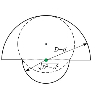
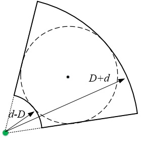
The outer region for the cases with dD𝑑𝐷d\leq D and d>D𝑑𝐷d>D is shown in Fig. 4. Placing the center of the sectors at the reference receiver in case dD𝑑𝐷d\leq D, two covering half-circles with radii d+D𝑑𝐷d+D and D2d2superscript𝐷2superscript𝑑2\sqrt{D^{2}-d^{2}} are considered. Also, in the case d>D𝑑𝐷d>D, we consider the sector with radii d+D𝑑𝐷d+D and dD𝑑𝐷d-D and the front angle 2φ02subscript𝜑02\varphi_{0} entangled between the two tangent lines. However, for the closest-selection strategy in the case d>D𝑑𝐷d>D, we can achieve a tighter bound by the following regions for 𝒜\𝐛(𝐨,Rc)\𝒜𝐛𝐨subscript𝑅c{\cal A}\backslash\mathbf{b}(\mathbf{o},R_{\text{c}}), which is the region including interfering transmitters. In the case Rc>d2D2subscript𝑅csuperscript𝑑2superscript𝐷2R_{\text{c}}>\sqrt{d^{2}-D^{2}}, the sector with the front angle equal to twice the intersection angle, i.e., 2φ1(Rc)2subscript𝜑1subscript𝑅c2\varphi_{1}(R_{\text{c}}), and radii Rcsubscript𝑅cR_{\text{c}} and D+d𝐷𝑑D+d is considered. In the case Rc<d2D2subscript𝑅csuperscript𝑑2superscript𝐷2R_{\text{c}}<\sqrt{d^{2}-D^{2}}, we consider two sectors with the front angle 2φ02subscript𝜑02\varphi_{0} and radii Rcsubscript𝑅cR_{\text{c}} and R1(φ1(Rc))subscript𝑅1subscript𝜑1subscript𝑅cR_{1}(\varphi_{1}(R_{\text{c}})) and with the front angle 2φ1(Rc)2subscript𝜑1subscript𝑅c2\varphi_{1}(R_{\text{c}}) and radii R1(φ1(Rc))subscript𝑅1subscript𝜑1subscript𝑅cR_{1}(\varphi_{1}(R_{\text{c}})) and D+d𝐷𝑑D+d.

Refer to caption
(a) dD𝑑𝐷d\leq D
Refer to caption
(b) d>D𝑑𝐷d>D
Figure 4: Outer bounds of 𝒜𝒜\cal A in the two cases dD𝑑𝐷d\leq D and d>D𝑑𝐷d>D.

In the following corollaries, we present the lower bounds on the LT of the interference for both strategies.

Corollary 1

With closest-selection, the LT of the interference given the serving distance Rcsubscript𝑅cR_{\text{c}} is lower bounded by

cbd(s|Rc)={A^d(s)ifdDand0<RcD2d2,B^d(s)ifdDandD2d2Rc<D+d,C^d(s)ifd>DanddDRc<d2D2,D^d(s)ifd>Dandd2D2Rc<D+d.\displaystyle{\cal L}_{{\cal I}_{\text{cb}}}^{d}(s|R_{\text{c}})=\left\{\begin{matrix}\hat{A}^{d}(s)&\text{if}\hskip 5.0pt{d\leq D}\hskip 5.0pt\text{and}\hskip 5.0pt{0<R_{\text{c}}\leq\sqrt{D^{2}-d^{2}}},\\ \hat{B}^{d}(s)&\text{if}\hskip 5.0pt{d\leq D}\hskip 5.0pt\text{and}\hskip 5.0pt{\sqrt{D^{2}-d^{2}}\leq R_{\text{c}}<D+d},\\ \hat{C}^{d}(s)&\text{if}\hskip 5.0pt{d>D}\hskip 5.0pt\text{and}\hskip 5.0pt{d-D\leq R_{\text{c}}<\sqrt{d^{2}-D^{2}}},\\ \hat{D}^{d}(s)&\text{if}\hskip 5.0pt{d>D}\hskip 5.0pt\text{and}\hskip 5.0pt{\sqrt{d^{2}-D^{2}}\leq R_{\text{c}}<D+d}.\end{matrix}\right. (35)

where A^d(s)superscript^𝐴𝑑𝑠\hat{A}^{d}(s), B^d(s)superscript^𝐵𝑑𝑠\hat{B}^{d}(s), C^d(s)superscript^𝐶𝑑𝑠\hat{C}^{d}(s), and D^d(s)superscript^𝐷𝑑𝑠\hat{D}^{d}(s) are defined as

A^d(s)=exp(πλ{(s,Rc)12(s,d+D)12(s,D2d2)}),superscript^𝐴𝑑𝑠𝜋𝜆𝑠subscript𝑅c12𝑠𝑑𝐷12𝑠superscript𝐷2superscript𝑑2\displaystyle\hat{A}^{d}(s)=\exp\biggl{(}\pi\lambda\left\{{\cal F}(s,R_{\text{c}})-\frac{1}{2}{\cal F}(s,d+D)-\frac{1}{2}{\cal F}(s,\sqrt{D^{2}-d^{2}})\right\}\biggr{)},\hskip 100.0pt (36)
B^d(s)=exp(π2λ{(s,Rc)(s,d+D)}),superscript^𝐵𝑑𝑠𝜋2𝜆𝑠subscript𝑅c𝑠𝑑𝐷\displaystyle\hat{B}^{d}(s)=\exp\left(\frac{\pi}{2}\lambda\Bigl{\{}{\cal F}(s,R_{\text{c}})-{\cal F}(s,d+D)\Bigr{\}}\right),\hskip 213.0pt (37)
C^d(s)=exp(λ{φ0(s,Rc)+(φ1(Rc)φ0)(s,R1(φ1(Rc)))φ1(Rc)(s,d+D)}),superscript^𝐶𝑑𝑠𝜆subscript𝜑0𝑠subscript𝑅csubscript𝜑1subscript𝑅csubscript𝜑0𝑠subscript𝑅1subscript𝜑1subscript𝑅csubscript𝜑1subscript𝑅c𝑠𝑑𝐷\displaystyle\hat{C}^{d}(s)=\exp\left(\lambda\Bigl{\{}\varphi_{0}{\cal F}(s,R_{\text{c}})+\left(\varphi_{1}(R_{\text{c}})-\varphi_{0}\right){\cal F}(s,R_{1}(\varphi_{1}(R_{\text{c}})))-\varphi_{1}(R_{\text{c}}){\cal F}(s,d+D)\Bigr{\}}\right), (38)
D^d(s)=exp(λφ1(Rc){(s,Rc)(s,d+D)}).superscript^𝐷𝑑𝑠𝜆subscript𝜑1subscript𝑅c𝑠subscript𝑅c𝑠𝑑𝐷\displaystyle\hat{D}^{d}(s)=\exp\left(\lambda\varphi_{1}(R_{\text{c}})\Bigl{\{}{\cal F}(s,R_{\text{c}})-{\cal F}(s,d+D)\Bigr{\}}\right).\hskip 190.0pt (39)
Proof:

The proof follows the same approach as in Appendix A, except that the disk is replaced with the regions given in Fig. 4. ∎

Corollary 2

With uniform-selection, the LT of the interference is lower bounded by

ubd(s)={E^d(s)ifdD,F^d(s)ifd>D.\displaystyle{\cal L}_{{\cal I}_{\text{ub}}}^{d}(s)=\left\{\begin{matrix}\hat{E}^{d}(s)&\text{if}\hskip 2.0ptd\leq D,\\ \hat{F}^{d}(s)&\text{if}\hskip 2.0ptd>D.\end{matrix}\right. (40)

where E^d(s)superscript^𝐸𝑑𝑠\hat{E}^{d}(s) and F^d(s)superscript^𝐹𝑑𝑠\hat{F}^{d}(s) are defined as

E^d(s)=exp(λπ2{(s,D2d2)+(s,D+d)})exp(λπD(D+d))(1exp(λπD(D+d)))(112D(D+d){(s,D2d2)+(s,D+d)}),superscript^𝐸𝑑𝑠𝜆𝜋2𝑠superscript𝐷2superscript𝑑2𝑠𝐷𝑑𝜆𝜋𝐷𝐷𝑑1𝜆𝜋𝐷𝐷𝑑112𝐷𝐷𝑑𝑠superscript𝐷2superscript𝑑2𝑠𝐷𝑑\displaystyle\hat{E}^{d}(s)=\frac{\exp\Bigl{(}-\frac{\lambda\pi}{2}\Bigl{\{}{\cal F}(s,\sqrt{D^{2}-d^{2}})+{\cal F}(s,D+d)\Bigr{\}}\Bigr{)}-\exp(-\lambda\pi D(D+d))}{(1-\exp(-\lambda\pi D(D+d)))\left(1-\frac{1}{2D(D+d)}\Bigl{\{}{\cal F}(s,\sqrt{D^{2}-d^{2}})+{\cal F}(s,D+d)\Bigr{\}}\right)}, (41)
F^d(s)=exp(λφ0{(s,d+D)(s,dD)})exp(4λdDφ0)(1exp(4λdDφ0))(114dD{(s,d+D)(s,dD)}).superscript^𝐹𝑑𝑠𝜆subscript𝜑0𝑠𝑑𝐷𝑠𝑑𝐷4𝜆𝑑𝐷subscript𝜑014𝜆𝑑𝐷subscript𝜑0114𝑑𝐷𝑠𝑑𝐷𝑠𝑑𝐷\displaystyle\hat{F}^{d}(s)=\frac{\exp\Bigl{(}-\lambda\varphi_{0}\Bigl{\{}{\cal F}(s,d+D)-{\cal F}(s,d-D)\Bigr{\}}\Bigr{)}-\exp(-4\lambda dD\varphi_{0})}{(1-\exp(-4\lambda dD\varphi_{0}))\left(1-\frac{1}{4dD}\Bigl{\{}{\cal F}(s,d+D)-{\cal F}(s,d-D)\Bigr{\}}\right)}.\hskip 60.0pt (42)
Proof:

The proof follows the same approach as in Appendix B, except that the disk is replaced with the regions given in Fig. 4. ∎

IV Multi-Cluster Wireless Networks

In this section, we extend our analysis to multi-cluster wireless networks. Closed-access and open-access receivers are investigated in Subsections IV.A and IV.B, respectively.

IV-A Closed-Access Receivers

For the analysis, we consider the reference closed-access receiver at the origin and add a cluster Φ𝐱osubscriptΦsubscript𝐱o{\Phi}_{\mathbf{x}_{\text{o}}} with intensity λ𝜆\lambda over the disk 𝐛(𝐱o,D)𝐛subscript𝐱o𝐷\mathbf{b}(\mathbf{x}_{\text{o}},D), where 𝐱onormsubscript𝐱o\|\mathbf{x}_{\text{o}}\| has PDF given in (1), to the network. Thanks to Slivnyak’s theorem [10, Thm. 8.10], this additional cluster and its receiver become the representative cluster and receiver under expectation over ΦΦ{\Phi}. This means this link’s performance corresponds to the average performance of all links in any realization of the network. Therefore, the serving transmitter under the closest-selection strategy is

𝐱c=argmin𝐲{Φ𝐱on(Φ𝐱o)>0}𝐲,subscript𝐱csubscript𝐲conditional-setsubscriptΦsubscript𝐱o𝑛subscriptΦsubscript𝐱o0norm𝐲\displaystyle{{\rm{\mathbf{x}}}}_{\text{c}}=\arg\mathop{\min}\limits_{{\mathbf{y}}\in\left\{{\Phi}_{\mathbf{x}_{\text{o}}}\mid n({\Phi}_{\mathbf{x}_{\text{o}}})>0\right\}}\|{{\mathbf{y}}}\|, (43)

while with the uniform-selection strategy, the serving transmitter is found by

𝐱u=Unif{Φ𝐱on(Φ𝐱o)>0}.subscript𝐱uUnifconditional-setsubscriptΦsubscript𝐱o𝑛subscriptΦsubscript𝐱o0\displaystyle{{\rm{\mathbf{x}}}}_{\text{u}}=\text{Unif}\left\{{\Phi}_{\mathbf{x}_{\text{o}}}\mid n({\Phi}_{\mathbf{x}_{\text{o}}})>0\right\}. (44)

Then, the SINR at the origin with distance 𝐱norm𝐱{\|\mathbf{x}\|} relative to the serving transmitter is

SINR=h𝐱𝐱ασ2+intra+inter,SINRsubscript𝐱superscriptnorm𝐱𝛼superscript𝜎2subscriptintrasubscriptinter\displaystyle\text{SINR}=\frac{{{h_{\mathbf{x}}}{{\|\mathbf{x}\|}^{-\alpha}}}}{{{\sigma^{2}}+{{\cal I}_{\text{intra}}}+{{\cal I}_{\text{inter}}}}}, (45)

where intra=𝐲Φ𝐱o\{𝐱}h𝐲𝐲αsubscriptintrasubscript𝐲\subscriptΦsubscript𝐱o𝐱subscript𝐲superscriptnorm𝐲𝛼{{\cal I}_{\text{intra}}}=\mathop{\sum}\limits_{\mathbf{y}\in{{\Phi}_{\mathbf{x}_{\text{o}}}}\backslash\left\{\mathbf{x}\right\}}{h_{\mathbf{y}}}{\|{\mathbf{y}}\|^{-\alpha}} denotes the intra-cluster interference caused by the transmitters inside the representative cluster, and inter=𝐲Φh𝐲𝐲αsubscriptintersubscript𝐲Φsubscript𝐲superscriptnorm𝐲𝛼{{\cal I}_{\text{inter}}}=\mathop{\sum}\limits_{{{\mathbf{y}}\in{{\Phi}}}}{h_{{\mathbf{y}}}}{\|{{\mathbf{y}}}\|^{-\alpha}} represents the inter-cluster interference caused by the transmitters outside the representative cluster.

Given the distance between the receiver and the center of the representative cluster, i.e., 𝐱onormsubscript𝐱o\|\mathbf{x}_{\text{o}}\|, the distributions of the distances Rc=𝐱csubscript𝑅cnormsubscript𝐱cR_{\text{c}}={\|\mathbf{x}_{\text{c}}\|} and Ru=𝐱usubscript𝑅unormsubscript𝐱uR_{\text{u}}={\|\mathbf{x}_{\text{u}}\|} are derived in Subsection III.B for the closest- and uniform-selection strategies, respectively. Also, the LT of the intra-cluster interference conditioned on 𝐱onormsubscript𝐱o\|\mathbf{x}_{\text{o}}\|, defined as the function intra𝐱osuperscriptsubscriptsubscriptintranormsubscript𝐱o{\cal L}_{{\cal I}_{\text{intra}}}^{\|\mathbf{x}_{\text{o}}\|}, is given by Theorems 1 and 2 for the closest-selection and uniform-selection strategies, relatively. The LT of the inter-cluster interference is also characterized in the following theorem.

Theorem 3

The LT of the inter-cluster interference intersubscriptinter{\cal I}_{\text{inter}} is

inter(s)=exp(2πλp(0D{1exp(λf(s,u))}udu+D{1exp(λg(s,u))}udu)),\displaystyle{\cal L}_{{\cal I}_{\text{inter}}}(s)=\exp\biggl{(}-2\pi\lambda_{\rm p}\biggr{(}\int\limits_{0}^{D}\Bigl{\{}1-\exp\left(-\lambda f(s,u)\right)\Bigr{\}}u\mathrm{d}u+\int\limits_{D}^{\infty}\Bigl{\{}1-\exp\left(-\lambda g(s,u)\right)\Bigr{\}}u\mathrm{d}u\biggr{)}\biggr{)}, (46)

where f(s,u)𝑓𝑠𝑢f(s,u) and g(s,u)𝑔𝑠𝑢g(s,u) are defined as

f(s,u)=0π(s,R2(u,θ))dθ,𝑓𝑠𝑢superscriptsubscript0𝜋𝑠subscript𝑅2𝑢𝜃differential-d𝜃\displaystyle f(s,u)=\int_{0}^{\pi}{\cal F}(s,{R_{2}(u,\theta)})\mathrm{d}\theta,\hskip 115.0pt (47)
g(s,u)=0φ2(u){(s,R2(u,θ))(s,R^2(u,θ))}dθ,𝑔𝑠𝑢superscriptsubscript0subscript𝜑2𝑢𝑠subscript𝑅2𝑢𝜃𝑠subscript^𝑅2𝑢𝜃differential-d𝜃\displaystyle g(s,u)=\int_{0}^{\varphi_{2}(u)}\Bigl{\{}{\cal F}(s,{R_{2}(u,\theta)})-{\cal F}(s,{\hat{R}_{2}(u,\theta)})\Bigr{\}}\mathrm{d}\theta, (48)

where φ2(u)=sin1(Du)subscript𝜑2𝑢superscript1𝐷𝑢\varphi_{2}(u)={\sin^{-1}}\left({\frac{D}{u}}\right), R2(u,θ)=ucos(θ)+D2u2sin2(θ)subscript𝑅2𝑢𝜃𝑢𝜃superscript𝐷2superscript𝑢2superscript2𝜃R_{2}(u,\theta)=u\cos\left(\theta\right)+\sqrt{{D^{2}}-{u^{2}}{{\sin}^{2}}\left(\theta\right)} and R^2(u,θ)=ucos(θ)D2u2sin2(θ)subscript^𝑅2𝑢𝜃𝑢𝜃superscript𝐷2superscript𝑢2superscript2𝜃\hat{R}_{2}(u,\theta)=u\cos\left(\theta\right)-\sqrt{D^{2}-{u^{2}}{{\sin}^{2}}\left(\theta\right)}.

Proof:

See Appendix C. ∎

Using the expressions derived for the intra- and inter-cluster interferences, the coverage probability under the closest-selection strategy is calculated by deconditioning as

PCca-c(β)=(n(Φ𝐱o)>0)(SINRc>βn(Φ𝐱o)>0)=(1exp(λπD2))×\displaystyle{P}_{\rm C}^{\text{ca-c}}(\beta)=\mathbb{P}(n({\Phi}_{\mathbf{x}_{\text{o}}})>0)\mathbb{P}(\text{SINR}_{\text{c}}>\beta\mid n({\Phi}_{\mathbf{x}_{\text{o}}})>0)=(1-\exp(-\lambda\pi D^{2}))\times
00(h𝐱rασ2+intra+inter>β)fRcv(r)f𝐱o(v)drdv,superscriptsubscript0superscriptsubscript0subscript𝐱superscript𝑟𝛼superscript𝜎2subscriptintrasubscriptinter𝛽superscriptsubscript𝑓subscript𝑅c𝑣𝑟subscript𝑓normsubscript𝐱o𝑣differential-d𝑟differential-d𝑣\displaystyle\int_{0}^{\infty}\int_{0}^{\infty}{\mathbb{P}}\left({\frac{{{h_{\mathbf{x}}}{{r}^{-\alpha}}}}{{{\sigma^{2}}+{{\cal I}_{\text{intra}}}+{{\cal I}_{\text{inter}}}}}>\beta}\right){f_{R_{\text{c}}}^{v}}\left(r\right){f_{\|\mathbf{x}_{\text{o}}\|}}\left(v\right)\mathrm{d}r\mathrm{d}v,\hskip 50.0pt (49)

where the conditional coverage probability is expressed as

(h𝐱rασ2+intra+inter>β)=exp(βσ2rα)cv(βrα|r)inter(βrα).subscript𝐱superscript𝑟𝛼superscript𝜎2subscriptintrasubscriptinter𝛽𝛽superscript𝜎2superscript𝑟𝛼superscriptsubscriptsubscriptc𝑣conditional𝛽superscript𝑟𝛼𝑟subscriptsubscriptinter𝛽superscript𝑟𝛼\displaystyle{\mathbb{P}}\left({\frac{{{h_{\mathbf{x}}}{{r}^{-\alpha}}}}{{{\sigma^{2}}+{{\cal I}_{\text{intra}}}+{{\cal I}_{\text{inter}}}}}>\beta}\right)=\exp\left(-{{{\beta{\sigma^{2}}}}}{r^{\alpha}}\right){\cal L}_{{\cal I}_{\text{c}}}^{v}\left({{\beta{r^{\alpha}}}}|r\right){\cal L}_{{\cal I}_{\text{inter}}}\left({{\beta{r^{\alpha}}}}\right). (50)

Then, according to the cases in Subsections III.B and C, (37) is given by

PCca-c(β)=0D0Dv2πλreλπr2exp(βσ2rα)cv(βrα|r)inter(βrα)f𝐱o(v)drdvsuperscriptsubscript𝑃Cca-c𝛽superscriptsubscript0𝐷superscriptsubscript0𝐷𝑣2𝜋𝜆𝑟superscript𝑒𝜆𝜋superscript𝑟2𝛽superscript𝜎2superscript𝑟𝛼superscriptsubscriptsubscriptc𝑣conditional𝛽superscript𝑟𝛼𝑟subscriptsubscriptinter𝛽superscript𝑟𝛼subscript𝑓normsubscript𝐱o𝑣differential-d𝑟differential-d𝑣\displaystyle{P}_{\rm C}^{\text{ca-c}}(\beta)=\int_{0}^{D}\int_{0}^{D-v}2\pi\lambda re^{-\lambda\pi r^{2}}\exp\left(-{{{\beta{\sigma^{2}}}}}{r^{\alpha}}\right){\cal L}_{\cal{I_{\text{c}}}}^{v}\left({{\beta{r^{\alpha}}}}|r\right){\cal L}_{\cal{I_{\text{inter}}}}\left({{\beta{r^{\alpha}}}}\right){f_{\|\mathbf{x}_{\text{o}}\|}}\left(v\right)\mathrm{d}r\mathrm{d}v
+0DDvD+vλv(r)reλv(r)exp(βσ2rα)cv(βrα|r)inter(βrα)f𝐱o(v)drdvsuperscriptsubscript0𝐷superscriptsubscript𝐷𝑣𝐷𝑣𝜆subscript𝑣𝑟𝑟superscript𝑒𝜆subscript𝑣𝑟𝛽superscript𝜎2superscript𝑟𝛼superscriptsubscriptsubscriptc𝑣conditional𝛽superscript𝑟𝛼𝑟subscriptsubscriptinter𝛽superscript𝑟𝛼subscript𝑓normsubscript𝐱o𝑣differential-d𝑟differential-d𝑣\displaystyle+\int_{0}^{D}\int_{D-v}^{D+v}\lambda\frac{{\partial{\cal B}_{v}(r)}}{{\partial r}}{e^{-\lambda{\cal B}_{v}(r)}}\exp\left(-{{{\beta{\sigma^{2}}}}}{r^{\alpha}}\right){\cal L}_{\cal I_{\text{c}}}^{v}\left({{\beta{r^{\alpha}}}}|r\right){\cal L}_{\cal{I_{\text{inter}}}}\left({{\beta{r^{\alpha}}}}\right){f_{\|\mathbf{x}_{\text{o}}\|}}\left(v\right)\mathrm{d}r\mathrm{d}v\hskip 4.0pt
+DvDD+vλv(r)reλv(r)exp(βσ2rα)cv(βrα|r)inter(βrα)f𝐱o(v)drdv.superscriptsubscript𝐷superscriptsubscript𝑣𝐷𝐷𝑣𝜆subscript𝑣𝑟𝑟superscript𝑒𝜆subscript𝑣𝑟𝛽superscript𝜎2superscript𝑟𝛼superscriptsubscriptsubscriptc𝑣conditional𝛽superscript𝑟𝛼𝑟subscriptsubscriptinter𝛽superscript𝑟𝛼subscript𝑓normsubscript𝐱o𝑣differential-d𝑟differential-d𝑣\displaystyle+\int_{D}^{\infty}\int_{v-D}^{D+v}\lambda\frac{{\partial{\cal B}_{v}(r)}}{{\partial r}}{e^{-\lambda{\cal B}_{v}(r)}}\exp\left(-{{{\beta{\sigma^{2}}}}}{r^{\alpha}}\right){\cal L}_{\cal I_{\text{c}}}^{v}\left({{\beta{r^{\alpha}}}}|r\right){\cal L}_{\cal{I_{\text{inter}}}}\left({{\beta{r^{\alpha}}}}\right){f_{\|\mathbf{x}_{\text{o}}\|}}\left(v\right)\mathrm{d}r\mathrm{d}v. (51)

Finally, the coverage probability with the uniform-selection strategy can be derived with the same procedure as in (37)-(39). It is given by

PCca-u(β)=(1eλπD2){0D0Dv2rD2exp(βσ2rα)uv(βrα)inter(βrα)f𝐱o(v)drdv\displaystyle{P}_{\text{\rm C}}^{\text{ca-u}}(\beta)=(1-e^{-\lambda\pi D^{2}})\biggl{\{}\int_{0}^{D}\int_{0}^{D-v}\frac{{2r}}{D^{2}}\exp\left(-{{{\beta{\sigma^{2}}}}}{r^{\alpha}}\right){\cal L}_{\cal{I_{\text{u}}}}^{v}\left({{\beta{r^{\alpha}}}}\right){\cal L}_{\cal{I_{\text{inter}}}}\left({{\beta{r^{\alpha}}}}\right){f_{\|\mathbf{x}_{\text{o}}\|}}\left(v\right)\mathrm{d}r\mathrm{d}v
+0DDvD+v1πD2v(r)rexp(βσ2rα)uv(βrα)inter(βrα)f𝐱o(v)drdvsuperscriptsubscript0𝐷superscriptsubscript𝐷𝑣𝐷𝑣1𝜋superscript𝐷2subscript𝑣𝑟𝑟𝛽superscript𝜎2superscript𝑟𝛼superscriptsubscriptsubscriptu𝑣𝛽superscript𝑟𝛼subscriptsubscriptinter𝛽superscript𝑟𝛼subscript𝑓normsubscript𝐱o𝑣differential-d𝑟differential-d𝑣\displaystyle+\int_{0}^{D}\int_{D-v}^{D+v}\frac{{1}}{\pi D^{2}}\frac{{\partial{\cal B}_{v}(r)}}{{\partial r}}\exp\left(-{{{\beta{\sigma^{2}}}}}{r^{\alpha}}\right){\cal L}_{\cal I_{\text{u}}}^{v}\left({{\beta{r^{\alpha}}}}\right){\cal L}_{\cal{I_{\text{inter}}}}\left({{\beta{r^{\alpha}}}}\right){f_{\|\mathbf{x}_{\text{o}}\|}}\left(v\right)\mathrm{d}r\mathrm{d}v\hskip 17.0pt
+DvDD+v1πD2v(r)rexp(βσ2rα)uv(βrα)inter(βrα)f𝐱o(v)drdv}.\displaystyle+\int_{D}^{\infty}\int_{v-D}^{D+v}\frac{{1}}{\pi D^{2}}\frac{{\partial{\cal B}_{v}(r)}}{{\partial r}}\exp\left(-{{{\beta{\sigma^{2}}}}}{r^{\alpha}}\right){\cal L}_{\cal I_{\text{u}}}^{v}\left({{\beta{r^{\alpha}}}}\right){\cal L}_{\cal{I_{\text{inter}}}}\left({{\beta{r^{\alpha}}}}\right){f_{\|\mathbf{x}_{\text{o}}\|}}\left(v\right)\mathrm{d}r\mathrm{d}v\biggr{\}}.\hskip 3.5pt (52)

IV-B Open-Access Receivers

Here, we only consider the closest-selection strategy. Note that there is no uniform-selection strategy in this case, since the number of transmitters is infinite. Therefore, the serving transmitter is

𝐱t=argmin𝐲Φ𝐲.subscript𝐱tsubscript𝐲Φnorm𝐲\displaystyle{{\rm{\mathbf{x}}}}_{\text{t}}=\arg\mathop{\min}\limits_{{\mathbf{y}}\in{\Phi}}\|{{\mathbf{y}}}\|. (53)

The distribution of the distance from the reference open-access receiver at the origin, i.e., Rt=𝐱tsubscript𝑅tnormsubscript𝐱tR_{\text{t}}={\|\mathbf{x}_{\text{t}}\|}, is given in the following theorem.

Theorem 4

The cumulative distribution function (CDF) of Rtsubscript𝑅t{R_{\text{t}}} is

FRt(r)={1exp(2πλp{(1exp(λπr2))(Dr)22+DrD+r(1exp(λu(r)))udu})if0r<D,1exp(2πλp{(1exp(λπD2))(rD)22+rDD+r(1exp(λu(r)))udu})ifrD.\displaystyle F_{R_{\text{t}}}(r)=\left\{\begin{matrix}1-\exp\biggl{(}-2\pi\lambda_{\rm p}\biggl{\{}\left(1-\exp\left(-\lambda\pi r^{2}\right)\right)\frac{(D-r)^{2}}{2}\\ +\int_{D-r}^{D+r}\left(1-\exp\left(-\lambda{\cal B}_{u}(r)\right)\right)u\mathrm{d}u\biggr{\}}\biggr{)}\hskip 30.0pt&\hskip 20.0pt\text{if}\hskip 5.0pt0\leq r<D,\\ 1-\exp\biggl{(}-2\pi\lambda_{\rm p}\biggl{\{}\left(1-\exp\left(-\lambda\pi D^{2}\right)\right)\frac{(r-D)^{2}}{2}\\ +\int_{r-D}^{D+r}\left(1-\exp\left(-\lambda{\cal B}_{u}(r)\right)\right)u\mathrm{d}u\biggr{\}}\biggr{)}\hskip 30.0pt&\text{if}\hskip 5.0ptr\geq D.\end{matrix}\right. (54)
Proof:

See Appendix D. ∎

Note that the contact distribution function of MCP is also derived in [28] using the probability generating functional (PGFL) of PCPs in [10, Cor. 4.13]. However, our approach is more tractable and leads to the result (42), which is much easier to numerically evaluate than [28, Thm. 1].

By taking the derivative of FRt(r)subscript𝐹subscript𝑅t𝑟F_{R_{\text{t}}}(r), using Leibniz integral rule, and some simplifications, the PDF of Rtsubscript𝑅tR_{\text{t}} can be obtained as

fRt(r)={2πλp{πλreλπr2(Dr)2+DrD+rλu(r)reλu(r)udu}×exp(2πλp{(1exp(λπr2))(Dr)22+DrD+r(1exp(λu(r)))udu})if0r<D,2πλp{rDD+rλu(r)reλu(r)udu}×exp(2πλp{(1exp(λπD2))(rD)22+rDD+r(1exp(λu(r)))udu})ifrD.\displaystyle{f_{R_{\text{t}}}}\left(r\right)=\left\{\begin{matrix}2\pi\lambda_{\rm p}\biggl{\{}\pi\lambda re^{-\lambda\pi r^{2}}(D-r)^{2}+\int_{D-r}^{D+r}\lambda\frac{{\partial{\cal B}_{u}(r)}}{{\partial r}}e^{-\lambda{\cal B}_{u}(r)}u\mathrm{d}u\biggr{\}}\\ \times\exp\biggl{(}-2\pi\lambda_{\rm p}\biggl{\{}\left(1-\exp\left(-\lambda\pi r^{2}\right)\right)\frac{(D-r)^{2}}{2}\hskip 47.0pt\\ +\int_{D-r}^{D+r}\left(1-\exp\left(-\lambda{\cal B}_{u}(r)\right)\right)u\mathrm{d}u\biggr{\}}\biggr{)}\hskip 71.0pt&\hskip 20.0pt\text{if}\hskip 5.0pt0\leq r<D,\\ 2\pi\lambda_{\rm p}\biggl{\{}\int_{r-D}^{D+r}\lambda\frac{{\partial{\cal B}_{u}(r)}}{{\partial r}}e^{-\lambda{\cal B}_{u}(r)}u\mathrm{d}u\biggr{\}}\hskip 105.0pt\\ \times\exp\biggl{(}-2\pi\lambda_{\rm p}\biggl{\{}\left(1-\exp\left(-\lambda\pi D^{2}\right)\right)\frac{(r-D)^{2}}{2}\hskip 42.0pt\\ +\int_{r-D}^{D+r}\left(1-\exp\left(-\lambda{\cal B}_{u}(r)\right)\right)u\mathrm{d}u\biggr{\}}\biggr{)}\hskip 70.0pt&\text{if}\hskip 5.0ptr\geq D.\end{matrix}\right. (55)

The SINR at the reference open-access receiver located at the origin is

SINRt=h𝐱tRtασ2+t,subscriptSINRtsubscriptsubscript𝐱tsuperscriptsubscript𝑅t𝛼superscript𝜎2subscriptt\displaystyle\text{SINR}_{\text{t}}=\frac{{{h_{\mathbf{x}_{\text{t}}}}{{R_{\text{t}}}^{-\alpha}}}}{{{\sigma^{2}}+{{\cal I}_{\text{t}}}}}, (56)

where t=𝐲Φ\{𝐱t}h𝐲𝐲αsubscripttsubscript𝐲\Φsubscript𝐱tsubscript𝐲superscriptnorm𝐲𝛼{{\cal I}_{\text{t}}}=\mathop{\sum}\limits_{\mathbf{y}\in{{\Phi}}\backslash\left\{\mathbf{x}_{\text{t}}\right\}}{h_{\mathbf{y}}}{\|{\mathbf{y}}\|^{-\alpha}} denotes the total interference caused by all transmitters except for the serving transmitter. The LT of the total interference tsubscriptt{\cal I}_{\text{t}} conditioned on the serving distance Rtsubscript𝑅tR_{\text{t}} is characterized in the following theorem.

Theorem 5

Conditioned on Rtsubscript𝑅tR_{\text{t}}, the LT of the total interference tsubscriptt{\cal I}_{\text{t}} is

t(s|Rt)={exp(2πλp{0DRt{1Au(s)}udu+DRtD2+Rt2{1Bu(s)}udu+D2+Rt2D+Rt{1Cu(s)}udu+D+Rt{1exp(λg(s,u))}udu})if0Rt<D,exp(2πλp{RtDD2+Rt2{1Bu(s)}udu+D2+Rt2D+Rt{1Cu(s)}udu+D+Rt{1exp(λg(s,u))}udu})ifRtD,\displaystyle{\cal L}_{{\cal I}_{\text{t}}}(s|R_{\text{t}})=\left\{\begin{matrix}\exp\biggl{(}-2\pi\lambda_{\rm p}\biggl{\{}\int_{0}^{D-R_{\text{t}}}\left\{1-{A}^{u}(s)\right\}u\mathrm{d}u\\ +\int_{D-R_{\text{t}}}^{\sqrt{D^{2}+R_{\text{t}}^{2}}}\left\{1-{B}^{u}(s)\right\}u\mathrm{d}u+\int_{\sqrt{D^{2}+R_{\text{t}}^{2}}}^{D+R_{\text{t}}}\left\{1-{C}^{u}(s)\right\}u\mathrm{d}u\\ +\int_{D+R_{\text{t}}}^{\infty}\left\{1-\exp\left(-\lambda g(s,u)\right)\right\}u\mathrm{d}u\biggr{\}}\biggr{)}\hskip 74.0pt&\text{if}\hskip 5.0pt0\leq R_{\text{t}}<D,\\ \exp\biggl{(}-2\pi\lambda_{\rm p}\biggl{\{}\int_{R_{\text{t}}-D}^{\sqrt{D^{2}+R_{\text{t}}^{2}}}\left\{1-{B}^{u}(s)\right\}u\mathrm{d}u\hskip 80.0pt\\ +\int_{\sqrt{D^{2}+R_{\text{t}}^{2}}}^{D+R_{\text{t}}}\left\{1-{C}^{u}(s)\right\}u\mathrm{d}u\hskip 125.0pt\\ +\int_{D+R_{\text{t}}}^{\infty}\left\{1-\exp\left(-\lambda g(s,u)\right)\right\}u\mathrm{d}u\biggr{\}}\biggr{)}\hskip 74.0pt&\text{if}\hskip 5.0ptR_{\text{t}}\geq D,\end{matrix}\right. (57)

where Au(s)superscript𝐴𝑢𝑠{A}^{u}(s), Bu(s)superscript𝐵𝑢𝑠{B}^{u}(s) and Cu(s)superscript𝐶𝑢𝑠{C}^{u}(s) are defined for a u𝑢u in (12), (13) and (14), respectively. Also, g(s,u)𝑔𝑠𝑢g(s,u) is given in (36).

Proof:

See Appendix E. ∎

Using Theorem 5 and (43) and the same procedure as in Subsection III.C, the coverage probability of the reference open-access receiver in multi-cluster wireless networks is found as

PCoa(β)=0exp(βσ2rα)t(βrα|r)fRt(r)dr.superscriptsubscript𝑃Coa𝛽superscriptsubscript0𝛽superscript𝜎2superscript𝑟𝛼subscriptsubscripttconditional𝛽superscript𝑟𝛼𝑟subscript𝑓subscript𝑅t𝑟differential-d𝑟\displaystyle{P}_{\rm C}^{\text{oa}}(\beta)=\int_{0}^{\infty}\exp\left(-{{{\beta{\sigma^{2}}}}}{r^{\alpha}}\right){\cal L}_{{\cal I}_{\text{t}}}\left({{\beta{r^{\alpha}}}}|r\right)f_{R_{\text{t}}}(r)\mathrm{d}r. (58)

V Numerical Results and Discussion

In this section, we provide analytical results for specific scenarios of single- and multi-cluster wireless networks. In addition, we discuss the results and provide key design insights.

V-A Single-Cluster Wireless Networks

We consider a scenario of single-cluster wireless networks in which the transmitters are distributed according to an FHPPP with intensity λ=0.01m2𝜆0.01superscriptm2\lambda=0.01\hskip 2.0pt\text{m}^{-2} in a disk with radius D=15m𝐷15mD=15\hskip 2.0pt\text{m} and evaluate the coverage probability results derived in Subsection III.C. Also, we evaluate the spectral efficiency, defined as τ=𝔼{log(1+SINR)}𝜏𝔼log1SINR\tau=\mathbb{E}\left\{\text{log}(1+\text{SINR})\right\}. The variance of the additive white Gaussian noise is set to σ2=0.0001superscript𝜎20.0001\sigma^{2}=0.0001. We further define the normalized (relative) distance δ=dD𝛿𝑑𝐷\delta=\frac{d}{D}. In the following, we study the impact of the path loss exponent and the distance of the receiver from the center of the disk on the coverage probability and the spectral efficiency. We also investigate the tightness of the bounds derived in Subsection III.D.

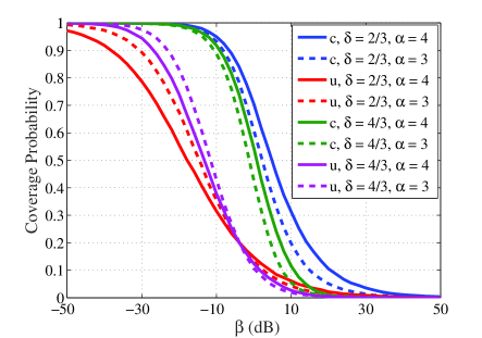
Effect of path loss exponent: The coverage probability as a function of the minimum required SINR β𝛽\beta is plotted in Fig. 5 for the closest- and uniform-selection strategies, considering δ=23𝛿23\delta=\frac{2}{3} and 4343\frac{4}{3} and α=3𝛼3\alpha=3 and 444. It is observed that the coverage probability is improved by increasing the path loss exponent. However, with the uniform-selection, a higher path loss exponent has a degrading effect when β𝛽\beta is lower than 55-5 dB. That is because the SINR exhibits a tradeoff as α𝛼\alpha increases. The power of both the desired and the interfering signals decrease, which can lead to an increase or decrease in the SINR, depending on β𝛽\beta and the other parameters. At a target coverage probability of 0.80.80.8, the (horizontal) gap between uniform- and closest-selection is about 202020 dB for α=3𝛼3\alpha=3 and 252525 dB for α=4𝛼4\alpha=4 in the case δ=23𝛿23\delta=\frac{2}{3} and 121212 dB for α=3𝛼3\alpha=3 and 181818 dB for α=4𝛼4\alpha=4 in the case δ=43𝛿43\delta=\frac{4}{3}.

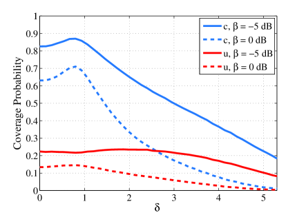
Effect of receiver distance from the center: The coverage probability as a function of the normalized distance δ𝛿\delta is studied in Fig. 6 for both selection strategies, α=4𝛼4\alpha=4 and β=5𝛽5\beta=-5 and 00 dB. It is observed that, depending on β𝛽\beta, there is an optimal value for the distance of the receiver, about 2D2𝐷2D for uniform-selection at β=5𝛽5\beta=-5 dB and 0.8D0.8𝐷0.8D for other cases, in terms of the coverage probability. This is due to the fact that the SINR has a tradeoff since the power of both the desired and the interfering signals decrease as the distance of the receiver to the center of the disk increases.

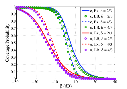
Tightness of the bounds: The tightness of the bounds on coverage probability derived in Subsection III.D is evaluated in Fig. 7 in the cases with different selection strategies and α=4𝛼4\alpha=4 and δ=23𝛿23\delta=\frac{2}{3} and 4343\frac{4}{3}. As observed, the bounds tightly approximate the performance in a broad range of SINR thresholds β𝛽\beta and for different positions of the receiver inside or outside the disk.

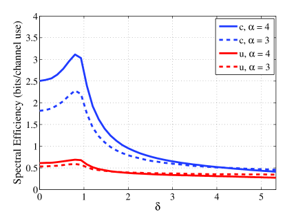
Spectral efficiency: The spectral efficiency as a function of δ𝛿\delta is shown in Fig. 8 for both selection strategies and α=3𝛼3\alpha=3 and 444. We analytically obtain the spectral efficiency from the coverage probability as, e.g., [8, Thm. 3]111Note that this is an upper bound on the actual spectral efficiency, since this formulation assumes that the transmitter knows all the fading coefficients between all other transmitters and the receiver, which would be a very generous assumption. A tighter lower bound could be found using the approach described in [33].

τq=0(log(1+SINRq)>t)dt=01ln2PCq(t)t+1dtbits/channel use,q={c,u}.formulae-sequencesuperscript𝜏𝑞superscriptsubscript0log1subscriptSINR𝑞𝑡differential-d𝑡superscriptsubscript01ln2superscriptsubscript𝑃C𝑞𝑡𝑡1differential-d𝑡bits/channel use𝑞cu\displaystyle\tau^{q}=\int_{0}^{\infty}\mathbb{P}(\text{log}\left(1+\text{SINR}_{q})>t\right)\mathrm{d}t=\int_{0}^{\infty}\frac{1}{\text{ln}2}\frac{{P}_{\rm C}^{q}\left(t\right)}{t+1}\mathrm{d}t\hskip 5.0pt\text{bits/channel use},\ q=\left\{\text{c},\text{u}\right\}. (59)

As observed, closest-selection achieves a much higher spectral efficiency than uniform-selection for different receiver distances. Also, there is a crossing point, whereby the spectral efficiency improves as α𝛼\alpha increases before reaching a distance for the receiver location outside the disk. Then, at higher distances, the reverse happens. This is intuitive because, at lower distances, the power of the interfering signals, which decreases with a higher path loss exponent, is the dominant factor on the SINR. On the other hand, at higher distances, the power of the desired signal, which increases with a smaller path loss exponent, dominates. Also, there may be an optimal value for the distance of the receiver in terms of the spectral efficiency. This is the result of the coverage probability behavior with the distance.
Refer to caption
Figure 5: Coverage probability as a function of the SINR threshold β𝛽\beta with δ=23𝛿23\delta=\frac{2}{3} and 4343\frac{4}{3}. c and u denote closest- and uniform-selection, respectively.
Refer to caption
Figure 6: Coverage probability as a function of normalized distance δ𝛿\delta with α=4𝛼4\alpha=4.
Refer to caption
Figure 7: On the tightness of the coverage probability lower bounds, α=4𝛼4\alpha=4. Ex and LB denote the exact result and the lower bound, respectively.
Refer to caption
Figure 8: Spectral efficiency as a function of normalized distance δ𝛿\delta.
Refer to caption
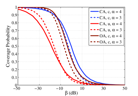
Figure 9: Coverage probability of the closed-access (CA) and open-access (OA) receiver as a function of threshold β𝛽\beta with δc=23subscript𝛿c23\delta_{\rm c}=\frac{2}{3}.
Refer to caption
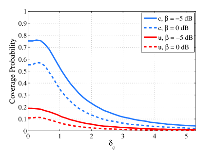
Figure 10: Coverage probability of the closed-access receiver as a function of normalized standard deviation δcsubscript𝛿c\delta_{\rm c} with α=4𝛼4\alpha=4.

V-B Multi-Cluster Wireless Networks

Here, we consider a multi-cluster wireless network where transmitters form an MCP with intensity λ=0.01m2𝜆0.01superscriptm2\lambda=0.01\hskip 2.0pt\text{m}^{-2} inside disks, all with equal radius D=15m𝐷15mD=15\hskip 2.0pt\text{m}, whose centers follow an HPPP with intensity λp=0.0004m2subscript𝜆p0.0004superscriptm2\lambda_{\rm p}=0.0004\hskip 2.0pt\text{m}^{-2}. Closed-access receivers are distributed with normal distribution with variance σc2superscriptsubscript𝜎c2\sigma_{\text{c}}^{2} around the cluster centers of transmitters. We further define normalized standard deviation δc=σcDsubscript𝛿csubscript𝜎c𝐷\delta_{\text{c}}=\frac{\sigma_{\text{c}}}{D}. In the following, the effects of the path loss exponent and variance of the normal distribution of closed-access receivers are assessed on the theoretical results derived in Subsections IV.A and IV.B.

Effect of path loss exponent: In Fig. 9, the coverage probability as a function of β𝛽\beta is plotted for the closest- and uniform-selection strategies in the case of closed-access receivers with δc=23subscript𝛿c23\delta_{\text{c}}=\frac{2}{3}. In this figure, the case of open-access receivers with the closest-selection strategy is also considered. Here, the results are presented for α=3𝛼3\alpha=3 and 444. As observed, a higher path loss exponent improves the coverage probability in practical minimum required SINRs.

Effect of variance of the normal distribution: The coverage probability as a function of the normalized standard deviation δcsubscript𝛿c\delta_{\text{c}} is shown in Fig. 10. Here, the results are presented for the closed-access receivers, considering α=4𝛼4\alpha=4 and β=5𝛽5\beta=-5 and 00 dB. It is observed that the coverage probability decreases as the standard deviation (or variance) of the normal distribution increases. It is intuitive because the probability of the event that the receiver is located farther from the representative transmitters increases with σcsubscript𝜎c\sigma_{\text{c}}.

VI Conclusion

In this paper, we developed a comprehensive tractable framework for the modeling and analysis of single- and multi-cluster wireless networks. Suitable for different wireless applications, we considered two strategies for a reference receiver to select a serving transmitter over a single-cluster wireless network: closest-selection and uniform-selection. Considering two types of receivers—closed-access receivers and open-access receivers—we then extended our modeling to multi-cluster wireless networks that are composed of distributed single-cluster wireless networks.

Using tools from stochastic geometry, we derived exact expressions for the coverage probability in the cases with different transmitter selection strategies and types of receivers in single- and multi-cluster wireless networks. We also proposed tight closed-form expressions bounding the coverage probability in the case of single-cluster wireless networks. Our analysis revealed that a higher path loss exponent improves the performance except when the receiver is outside and relatively far from its cluster of transmitters. In addition, although an increase in the distance of the receiver to the center of the cluster typically degrades the performance, there exists a location with optimal performance for the receiver. Also, the closest-selection strategy significantly outperforms the uniform-selection strategy.

Appendix A Proof of Theorem 1

The LT of the interference, given the serving distance Rcsubscript𝑅cR_{\text{c}}, is calculated as

cd(s|Rc)=𝔼{exp(s𝐲Φ\{𝐱c}h𝐲𝐲α)n(Φ)>0}superscriptsubscriptsubscriptc𝑑conditional𝑠subscript𝑅c𝔼𝑠subscript𝐲\Φsubscript𝐱csubscript𝐲superscriptnorm𝐲𝛼ket𝑛Φ0\displaystyle{\cal L}_{{\cal I}_{\text{c}}}^{d}(s|R_{\text{c}})=\mathbb{E}\left\{\exp\left(-s\mathop{\sum}\nolimits_{\mathbf{y}\in{\Phi}\backslash\left\{\mathbf{x}_{\text{c}}\right\}}{h_{\mathbf{y}}}{{\|\mathbf{y}\|}^{-\alpha}}\right)\mid n({\Phi})>0\right\}\hskip 130.0pt
=𝔼{𝐲Φ\{𝐱c}exp(sh𝐲𝐲α)n(Φ)>0}=(a)𝔼{𝐲Φ\{𝐱c}11+s𝐲αn(Φ)>0}absent𝔼subscriptproduct𝐲\Φsubscript𝐱c𝑠subscript𝐲superscriptnorm𝐲𝛼ket𝑛Φ0superscript𝑎𝔼conditional-setsubscriptproduct𝐲\Φsubscript𝐱c11𝑠superscriptnorm𝐲𝛼𝑛Φ0\displaystyle=\mathbb{E}\Biggl{\{}\mathop{\prod}\limits_{\mathbf{y}\in{\Phi}\backslash\left\{\mathbf{x}_{\text{c}}\right\}}\exp\left(-s{h_{\mathbf{y}}}{{\|\mathbf{y}\|}^{-\alpha}}\right)\mid n({\Phi})>0\Biggr{\}}\stackrel{{\scriptstyle(a)}}{{=}}\mathbb{E}\Biggl{\{}\mathop{\prod}\limits_{\mathbf{y}\in{\Phi}\backslash\left\{\mathbf{x}_{\text{c}}\right\}}\frac{1}{{1+s{{\|\mathbf{y}\|}^{-\alpha}}}}\mid n({\Phi})>0\Biggr{\}}
=(b)exp(λ𝒜\𝐛(𝐨,Rc)(111+s𝐲α)d𝐲),superscript𝑏absent𝜆subscript\𝒜𝐛𝐨subscript𝑅c111𝑠superscriptnorm𝐲𝛼differential-d𝐲\displaystyle\stackrel{{\scriptstyle(b)}}{{=}}\exp\left(-\lambda\int_{{\cal A}\backslash\mathbf{b}(\mathbf{o},R_{\text{c}})}\left(1-\frac{1}{{1+s{{\|\mathbf{y}\|}^{-\alpha}}}}\right)\mathrm{d}\mathbf{y}\right),\hskip 190.5pt (60)

where (a)𝑎(a) is obtained by h𝐲exp(1)similar-tosubscript𝐲1h_{\mathbf{y}}\sim\exp(1) and (b)𝑏(b) follows from the PGFL of the PPP [10, Thm. 4.9] and the fact that interfering nodes are farther away than Rcsubscript𝑅cR_{\text{c}}. Having a non-empty intersection between 𝒜𝒜{\cal A} and 𝐛(𝐨,Rc)𝐛𝐨subscript𝑅c\mathbf{b}(\mathbf{o},R_{\text{c}}), to compute (48), there are two types for d<D𝑑𝐷d<D (Case 1) and two types for d>D𝑑𝐷d>D (Case 2) to convert from Cartesian to polar coordinates. In fact, each type denotes a special form of 𝒜\𝐛(𝐨,Rc)\𝒜𝐛𝐨subscript𝑅c{\cal A}\backslash\mathbf{b}(\mathbf{o},R_{\text{c}}) that can be represented by polar coordinates uniquely.

Case 1: We have two different types for the case d<D𝑑𝐷d<D as follows.

Type 1: If 𝒜𝐛(𝐨,Rc)=𝐛(𝐨,Rc)𝒜𝐛𝐨subscript𝑅c𝐛𝐨subscript𝑅c{\cal A}\cap\mathbf{b}(\mathbf{o},R_{\text{c}})=\mathbf{b}(\mathbf{o},R_{\text{c}}) as given in Fig. 2(b), i.e., 0Rc<Dd0subscript𝑅c𝐷𝑑0\leq R_{\text{c}}<D-d, then

cd(s|Rc)=exp(λ02π0R1(θ)(111+sxα)xdxdθ+λ02π0Rc(111+sxα)xdxdθ).superscriptsubscriptsubscriptc𝑑conditional𝑠subscript𝑅c𝜆superscriptsubscript02𝜋superscriptsubscript0subscript𝑅1𝜃111𝑠superscript𝑥𝛼𝑥differential-d𝑥differential-d𝜃𝜆superscriptsubscript02𝜋superscriptsubscript0subscript𝑅c111𝑠superscript𝑥𝛼𝑥differential-d𝑥differential-d𝜃\displaystyle{\cal L}_{{\cal I}_{\text{c}}}^{d}(s|R_{\text{c}})=\exp\biggl{(}-\lambda\int\limits_{0}^{2\pi}\int\limits_{0}^{R_{1}(\theta)}\left(1-\frac{1}{{1+s{{x}^{-\alpha}}}}\right)x\mathrm{d}x\mathrm{d}\theta+\lambda\int\limits_{0}^{2\pi}\int\limits_{0}^{R_{\text{c}}}\left(1-\frac{1}{{1+s{{x}^{-\alpha}}}}\right)x\mathrm{d}x\mathrm{d}\theta\biggr{)}. (61)

This can be simplified to

cd(s|Rc)=exp(2πλ0Rcx1+xαsdxλ02π0R1(θ)x1+xαsdxdθ)superscriptsubscriptsubscriptc𝑑conditional𝑠subscript𝑅c2𝜋𝜆superscriptsubscript0subscript𝑅c𝑥1superscript𝑥𝛼𝑠differential-d𝑥𝜆superscriptsubscript02𝜋superscriptsubscript0subscript𝑅1𝜃𝑥1superscript𝑥𝛼𝑠differential-d𝑥differential-d𝜃\displaystyle{\cal L}_{{\cal I}_{\text{c}}}^{d}(s|R_{\text{c}})=\exp\left(2\pi\lambda\int_{0}^{R_{\text{c}}}\frac{x}{{1+\frac{{{x^{\alpha}}}}{s}}}\mathrm{d}x-\lambda\int_{0}^{2\pi}\int_{0}^{R_{1}(\theta)}\frac{x}{{1+\frac{{{x^{\alpha}}}}{s}}}\mathrm{d}x\mathrm{d}\theta\right)
=(c)exp(πλ(s,Rc)λ0π(s,R1(θ))dθ),superscript𝑐absent𝜋𝜆𝑠subscript𝑅c𝜆superscriptsubscript0𝜋𝑠subscript𝑅1𝜃differential-d𝜃\displaystyle\stackrel{{\scriptstyle(c)}}{{=}}\exp\left(\pi\lambda{\cal F}(s,R_{\text{c}})-{\lambda}\int_{0}^{\pi}{\cal F}(s,R_{1}(\theta))\mathrm{d}\theta\right),\hskip 66.0pt (62)

where (c)𝑐(c) follows from replacing xαsuperscript𝑥𝛼x^{\alpha} with u𝑢u and calculating the corresponding integral based on the formula [32, (3.194.1)] which uses the Gauss hypergeometric function F12subscriptsubscript𝐹12{}_{2}{F_{1}}.

Type 2: If 𝒜𝐛(𝐨,Rc)𝐛(𝐨,Rc)𝒜𝐛𝐨subscript𝑅c𝐛𝐨subscript𝑅c{\cal A}\cap\mathbf{b}(\mathbf{o},R_{\text{c}})\neq\mathbf{b}(\mathbf{o},R_{\text{c}}) as given in Fig. 2(a), i.e., DdRc<D+d𝐷𝑑subscript𝑅c𝐷𝑑D-d\leq R_{\text{c}}<D+d, then

cd(s|Rc)=exp(λφ1(Rc)φ1(Rc)RcR1(θ)(111+sxα)xdxdθ)superscriptsubscriptsubscriptc𝑑conditional𝑠subscript𝑅c𝜆superscriptsubscriptsubscript𝜑1subscript𝑅csubscript𝜑1subscript𝑅csuperscriptsubscriptsubscript𝑅csubscript𝑅1𝜃111𝑠superscript𝑥𝛼𝑥differential-d𝑥differential-d𝜃\displaystyle{\cal L}_{{\cal I}_{\text{c}}}^{d}(s|R_{\text{c}})=\exp\left(-\lambda\int_{-\varphi_{1}(R_{\text{c}})}^{\varphi_{1}(R_{\text{c}})}\int_{R_{\text{c}}}^{{R}_{1}(\theta)}\left(1-\frac{1}{{1+s{{x}^{-\alpha}}}}\right)x\mathrm{d}x\mathrm{d}\theta\right)
=exp(λ0φ1(Rc){(s,R1(θ))(s,Rc)}dθ).absent𝜆superscriptsubscript0subscript𝜑1subscript𝑅c𝑠subscript𝑅1𝜃𝑠subscript𝑅cdifferential-d𝜃\displaystyle=\exp\biggl{(}-\lambda\int_{0}^{\varphi_{1}(R_{\text{c}})}\Bigl{\{}{\cal F}(s,R_{1}(\theta))-{\cal F}(s,R_{\text{c}})\Bigr{\}}\mathrm{d}\theta\biggr{)}.\hskip 17.0pt (63)

Case 2: As observed from Fig. 2(c) for the case d>D𝑑𝐷d>D, we have two different types of the LT of the interference depending on whether or not, at an angle, the lower boundary of 𝒜𝒜\cal A within the two tangent lines crossing the origin is included in the boundary of 𝒜\𝐛(𝐨,Rc)\𝒜𝐛𝐨subscript𝑅c{\cal A}\backslash\mathbf{b}(\mathbf{o},R_{\text{c}}).

Type 1: Since the intersection angle φ1(r)subscript𝜑1𝑟\varphi_{1}(r) at r=d2D2𝑟superscript𝑑2superscript𝐷2r=\sqrt{d^{2}-D^{2}} is equal to the angle of the tangent lines φ0subscript𝜑0\varphi_{0}, if dD<Rc<d2D2𝑑𝐷subscript𝑅csuperscript𝑑2superscript𝐷2d-D<R_{\text{c}}<\sqrt{d^{2}-D^{2}}, we have

cd(s|Rc)=exp(λ{φ0φ1(Rc)R^1(θ)R1(θ)(111+sxα)xdxdθ\displaystyle{\cal L}_{{\cal I}_{\text{c}}}^{d}(s|R_{\text{c}})=\exp\biggl{(}-\lambda\biggl{\{}\int_{-\varphi_{0}}^{-\varphi_{1}(R_{\text{c}})}\int_{\hat{R}_{1}(\theta)}^{R_{1}(\theta)}\left(1-\frac{1}{{1+s{{x}^{-\alpha}}}}\right)x\mathrm{d}x\mathrm{d}\theta\hskip 130.0pt
+φ1(Rc)φ1(Rc)RcR1(θ)(111+sxα)xdxdθ+φ1(Rc)φ0R^1(θ)R1(θ)(111+sxα)xdxdθ})\displaystyle+\int_{-\varphi_{1}(R_{\text{c}})}^{\varphi_{1}(R_{\text{c}})}\int_{R_{\text{c}}}^{R_{1}(\theta)}\left(1-\frac{1}{{1+s{{x}^{-\alpha}}}}\right)x\mathrm{d}x\mathrm{d}\theta+\int_{\varphi_{1}(R_{\text{c}})}^{\varphi_{0}}\int_{\hat{R}_{1}(\theta)}^{R_{1}(\theta)}\left(1-\frac{1}{{1+s{{x}^{-\alpha}}}}\right)x\mathrm{d}x\mathrm{d}\theta\biggr{\}}\biggr{)}\hskip 5.0pt
=exp(λφ1(Rc)φ0{(s,R1(θ))(s,R^1(θ))}dθλ0φ1(Rc){(s,R1(θ))(s,Rc)}dθ).absent𝜆superscriptsubscriptsubscript𝜑1subscript𝑅csubscript𝜑0𝑠subscript𝑅1𝜃𝑠subscript^𝑅1𝜃differential-d𝜃𝜆superscriptsubscript0subscript𝜑1subscript𝑅c𝑠subscript𝑅1𝜃𝑠subscript𝑅cdifferential-d𝜃\displaystyle=\exp\biggl{(}-\lambda\int\limits_{\varphi_{1}(R_{\text{c}})}^{\varphi_{0}}\Bigl{\{}{\cal F}(s,R_{1}(\theta))-{\cal F}(s,\hat{R}_{1}(\theta))\Bigr{\}}\mathrm{d}\theta-{\lambda}\int\limits_{0}^{\varphi_{1}(R_{\text{c}})}\Bigl{\{}{\cal F}(s,R_{1}(\theta))-{\cal F}(s,R_{\text{c}})\Bigr{\}}\mathrm{d}\theta\biggr{)}. (64)

Type 2: If d2D2<Rc<d+Dsuperscript𝑑2superscript𝐷2subscript𝑅c𝑑𝐷\sqrt{d^{2}-D^{2}}<R_{\text{c}}<d+D, then

cd(s|Rc)=exp(λφ1(Rc)φ1(Rc)RcR1(θ)(111+sxα)xdxdθ)superscriptsubscriptsubscriptc𝑑conditional𝑠subscript𝑅c𝜆superscriptsubscriptsubscript𝜑1subscript𝑅csubscript𝜑1subscript𝑅csuperscriptsubscriptsubscript𝑅csubscript𝑅1𝜃111𝑠superscript𝑥𝛼𝑥differential-d𝑥differential-d𝜃\displaystyle{\cal L}_{{\cal I}_{\text{c}}}^{d}(s|R_{\text{c}})=\exp\left(-\lambda\int_{-\varphi_{1}(R_{\text{c}})}^{\varphi_{1}(R_{\text{c}})}\int_{R_{\text{c}}}^{R_{1}(\theta)}\left(1-\frac{1}{{1+s{{x}^{-\alpha}}}}\right)x\mathrm{d}x\mathrm{d}\theta\right)
=exp(λ0φ1(Rc){(s,R1(θ))(s,Rc)}dθ).absent𝜆superscriptsubscript0subscript𝜑1subscript𝑅c𝑠subscript𝑅1𝜃𝑠subscript𝑅cdifferential-d𝜃\displaystyle=\exp\biggl{(}-{\lambda}\int_{0}^{\varphi_{1}(R_{\text{c}})}\Bigl{\{}{\cal F}(s,R_{1}(\theta))-{\cal F}(s,R_{\text{c}})\Bigr{\}}\mathrm{d}\theta\biggr{)}.\hskip 17.0pt (65)

Appendix B Proof of Theorem 2

The LT of the interference is

ud(s)=𝔼{exp(s𝐲Φ\{𝐱u}h𝐲𝐲α)n(Φ)>0}superscriptsubscriptsubscriptu𝑑𝑠𝔼𝑠subscript𝐲\Φsubscript𝐱usubscript𝐲superscriptnorm𝐲𝛼ket𝑛Φ0\displaystyle{\cal L}_{{\cal I}_{\text{u}}}^{d}(s)=\mathbb{E}\left\{\exp\left(-s\mathop{\sum}\nolimits_{\mathbf{y}\in{\Phi}\backslash\left\{\mathbf{x}_{\text{u}}\right\}}{h_{\mathbf{y}}}{{\|\mathbf{y}\|}^{-\alpha}}\right)\mid n({\Phi})>0\right\}\hskip 150.0pt
=𝔼{𝐲Φ\{𝐱u}exp(sh𝐲𝐲α)n(Φ)>0}=(a)𝔼{𝐲Φ\{𝐱u}11+s𝐲αn(Φ)>0}absent𝔼subscriptproduct𝐲\Φsubscript𝐱u𝑠subscript𝐲superscriptnorm𝐲𝛼ket𝑛Φ0superscript𝑎𝔼conditional-setsubscriptproduct𝐲\Φsubscript𝐱u11𝑠superscriptnorm𝐲𝛼𝑛Φ0\displaystyle=\mathbb{E}\Biggl{\{}\mathop{\prod}\limits_{\mathbf{y}\in{\Phi}\backslash\left\{\mathbf{x}_{\text{u}}\right\}}\exp\left(-s{h_{\mathbf{y}}}{{\|\mathbf{y}\|}^{-\alpha}}\right)\mid n({\Phi})>0\Biggr{\}}\stackrel{{\scriptstyle(a)}}{{=}}\mathbb{E}\Biggl{\{}\mathop{\prod}\limits_{\mathbf{y}\in{\Phi}\backslash\left\{\mathbf{x}_{\text{u}}\right\}}\frac{1}{{1+s{{\|\mathbf{y}\|}^{-\alpha}}}}\mid n({\Phi})>0\Biggr{\}}
=(b)𝔼{(011+sxαfRu(x)dx)n(Φ)1n(Φ)>0}superscript𝑏absent𝔼conditional-setsuperscriptsuperscriptsubscript011𝑠superscript𝑥𝛼subscript𝑓subscript𝑅u𝑥differential-d𝑥𝑛Φ1𝑛Φ0\displaystyle\stackrel{{\scriptstyle(b)}}{{=}}\mathbb{E}\Biggl{\{}\left(\int_{0}^{\infty}\frac{1}{{1+s{{x}^{-\alpha}}}}f_{R_{\text{u}}}(x)\mathrm{d}x\right)^{n({\Phi})-1}\mid n({\Phi})>0\Biggr{\}}\hskip 170.0pt
=(c)k=1exp(λπD2)(λπD2)kk!(1exp(λπD2))(011+sxαfRu(x)dx)k1superscript𝑐absentsuperscriptsubscript𝑘1𝜆𝜋superscript𝐷2superscript𝜆𝜋superscript𝐷2𝑘𝑘1𝜆𝜋superscript𝐷2superscriptsuperscriptsubscript011𝑠superscript𝑥𝛼subscript𝑓subscript𝑅u𝑥differential-d𝑥𝑘1\displaystyle\stackrel{{\scriptstyle(c)}}{{=}}\mathop{\sum}\limits_{k=1}^{\infty}\frac{\exp(-\lambda\pi D^{2})(\lambda\pi D^{2})^{k}}{k!(1-\exp(-\lambda\pi D^{2}))}\left(\int_{0}^{\infty}\frac{1}{{1+s{{x}^{-\alpha}}}}f_{R_{\text{u}}}(x)\mathrm{d}x\right)^{k-1}\hskip 133.0pt
=1(1exp(λπD2))011+sxαfRu(x)dx×\displaystyle=\frac{1}{(1-\exp(-\lambda\pi D^{2}))\int_{0}^{\infty}\frac{1}{{1+s{{x}^{-\alpha}}}}f_{R_{\text{u}}}(x)\mathrm{d}x}\times\hskip 205.0pt
(k=0exp(λπD2)(λπD2)kk!(011+sxαfRu(x)dx)kexp(λπD2))superscriptsubscript𝑘0𝜆𝜋superscript𝐷2superscript𝜆𝜋superscript𝐷2𝑘𝑘superscriptsuperscriptsubscript011𝑠superscript𝑥𝛼subscript𝑓subscript𝑅u𝑥differential-d𝑥𝑘𝜆𝜋superscript𝐷2\displaystyle\left(\mathop{\sum}\limits_{k=0}^{\infty}\frac{\exp(-\lambda\pi D^{2})(\lambda\pi D^{2})^{k}}{k!}\left(\int_{0}^{\infty}\frac{1}{{1+s{{x}^{-\alpha}}}}f_{R_{\text{u}}}(x)\mathrm{d}x\right)^{k}-\exp(-\lambda\pi D^{2})\right)\hskip 50.0pt
=(d)exp(λπD2)(1exp(λπD2))011+sxαfRu(x)dx(exp(λπD2011+sxαfRu(x)dx)1),superscript𝑑absent𝜆𝜋superscript𝐷21𝜆𝜋superscript𝐷2superscriptsubscript011𝑠superscript𝑥𝛼subscript𝑓subscript𝑅u𝑥differential-d𝑥𝜆𝜋superscript𝐷2superscriptsubscript011𝑠superscript𝑥𝛼subscript𝑓subscript𝑅u𝑥differential-d𝑥1\displaystyle\stackrel{{\scriptstyle(d)}}{{=}}\frac{\exp(-\lambda\pi D^{2})}{(1-\exp(-\lambda\pi D^{2}))\int\limits_{0}^{\infty}\frac{1}{{1+s{{x}^{-\alpha}}}}f_{R_{\text{u}}}(x)\mathrm{d}x}\Biggl{(}\exp\Biggl{(}\lambda\pi D^{2}\int\limits_{0}^{\infty}\frac{1}{{1+s{{x}^{-\alpha}}}}f_{R_{\text{u}}}(x)\mathrm{d}x\Biggr{)}-1\Biggr{)}, (66)

where fRudsuperscriptsubscript𝑓subscript𝑅u𝑑{f_{R_{\text{u}}}^{d}} is the PDF of Rusubscript𝑅uR_{\text{u}} obtained from the distributions in (9)-(10) and (a)𝑎(a) is found by h𝐲exp(1)similar-tosubscript𝐲1h_{\mathbf{y}}\sim\exp(1). Also, (b)𝑏(b) follows from the fact that conditioned on n(Φ)𝑛Φn(\Phi), ΦΦ\Phi is a BPP where the distance 𝐲norm𝐲\|\mathbf{y}\| of each point is i.i.d. with distribution fRudsuperscriptsubscript𝑓subscript𝑅u𝑑f_{R_{\text{u}}}^{d}, (c)𝑐(c) follows from (n(Φ)=kn(Φ)>0)=exp(λπD2)(λπD2)kk!(1exp(λπD2))𝑛Φ𝑘ket𝑛Φ0𝜆𝜋superscript𝐷2superscript𝜆𝜋superscript𝐷2𝑘𝑘1𝜆𝜋superscript𝐷2\mathbb{P}(n({\Phi})=k\mid n({\Phi})>0)=\frac{\exp(-\lambda\pi D^{2})(\lambda\pi D^{2})^{k}}{k!(1-\exp(-\lambda\pi D^{2}))}, and (d)𝑑(d) is found by the moment-generating function (MGF) of a Poisson random variable with mean λπD2𝜆𝜋superscript𝐷2\lambda\pi D^{2} and some simplifications. According to (9)-(10), there are two cases to compute the integral:

Case 1: If dD𝑑𝐷d\leq D, then

011+sxαfRu(x)dx=0Dd11+sxα2xD2dx+DdD+d11+sxα1πD2d(x)xdx.superscriptsubscript011𝑠superscript𝑥𝛼subscript𝑓subscript𝑅u𝑥differential-d𝑥superscriptsubscript0𝐷𝑑11𝑠superscript𝑥𝛼2𝑥superscript𝐷2differential-d𝑥superscriptsubscript𝐷𝑑𝐷𝑑11𝑠superscript𝑥𝛼1𝜋superscript𝐷2subscript𝑑𝑥𝑥differential-d𝑥\displaystyle\int_{0}^{\infty}\frac{1}{{1+s{{x}^{-\alpha}}}}f_{R_{\text{u}}}(x)\mathrm{d}x=\int_{0}^{D-d}\frac{1}{{1+s{{x}^{-\alpha}}}}\frac{2x}{D^{2}}\mathrm{d}x+\int_{D-d}^{D+d}\frac{1}{{1+s{{x}^{-\alpha}}}}\frac{{1}}{\pi D^{2}}\frac{{\partial{\cal B}_{d}(x)}}{{\partial x}}\mathrm{d}x. (67)

Case 2: If d>D𝑑𝐷d>D, then

011+sxαfRu(x)dx=dDD+d11+sxα1πD2d(x)xdx.superscriptsubscript011𝑠superscript𝑥𝛼subscript𝑓subscript𝑅u𝑥differential-d𝑥superscriptsubscript𝑑𝐷𝐷𝑑11𝑠superscript𝑥𝛼1𝜋superscript𝐷2subscript𝑑𝑥𝑥differential-d𝑥\displaystyle\int_{0}^{\infty}\frac{1}{{1+s{{x}^{-\alpha}}}}f_{R_{\text{u}}}(x)\mathrm{d}x=\int_{d-D}^{D+d}\frac{1}{{1+s{{x}^{-\alpha}}}}\frac{{1}}{\pi D^{2}}\frac{{\partial{\cal B}_{d}(x)}}{{\partial x}}\mathrm{d}x. (68)

Appendix C Proof of Theorem 3

The LT of the inter-cluster interference is

inter(s)=𝔼{exp(s𝐱Φp𝐲Φ𝐱h𝐲𝐲α)}=𝔼{𝐱Φp𝐲Φ𝐱exp(sh𝐲𝐲α)}subscriptsubscriptinter𝑠𝔼𝑠subscript𝐱subscriptΦpsubscript𝐲subscriptΦ𝐱subscript𝐲superscriptnorm𝐲𝛼𝔼subscriptproduct𝐱subscriptΦpsubscriptproduct𝐲subscriptΦ𝐱𝑠subscript𝐲superscriptnorm𝐲𝛼\displaystyle{\cal L}_{{\cal I}_{\text{inter}}}(s)=\mathbb{E}\Biggl{\{}\exp\Biggl{(}-s\mathop{\sum}\limits_{\mathbf{x}\in{\Phi}_{\rm p}}\mathop{\sum}\limits_{{{\mathbf{y}}\in{{\Phi}_{\mathbf{x}}}}}{h_{{\mathbf{y}}}}{\|{{\mathbf{y}}}\|^{-\alpha}}\Biggr{)}\Biggr{\}}=\mathbb{E}\Biggl{\{}\mathop{\prod}\limits_{{\mathbf{x}\in{\Phi}_{\rm p}}}\mathop{\prod}\limits_{\mathbf{y}\in{\Phi}_{\mathbf{x}}}\exp\left(-s{h_{{\mathbf{y}}}}{\|{{\mathbf{y}}}\|^{-\alpha}}\right)\Biggr{\}}\hskip 13.0pt
=(a)𝔼{𝐱Φp𝐲Φ𝐱11+s𝐲α}=(b)𝔼{𝐱Φp𝐳Φo11+s𝐳+𝐱α}superscript𝑎absent𝔼subscriptproduct𝐱subscriptΦpsubscriptproduct𝐲subscriptΦ𝐱11𝑠superscriptnorm𝐲𝛼superscript𝑏𝔼subscriptproduct𝐱subscriptΦpsubscriptproduct𝐳subscriptΦo11𝑠superscriptnorm𝐳𝐱𝛼\displaystyle\stackrel{{\scriptstyle(a)}}{{=}}\mathbb{E}\Biggl{\{}\mathop{\prod}\limits_{{\mathbf{x}\in{\Phi}_{\rm p}}}\mathop{\prod}\limits_{\mathbf{y}\in{\Phi}_{\mathbf{x}}}\frac{1}{{1+s{{\|\mathbf{y}\|}^{-\alpha}}}}\Biggr{\}}\stackrel{{\scriptstyle(b)}}{{=}}\mathbb{E}\left\{\mathop{\prod}\limits_{\mathbf{x}\in{\Phi}_{\rm p}}\mathop{\prod}\limits_{\mathbf{z}\in{\Phi}_{\text{o}}}\frac{1}{{1+s{{\|\mathbf{z}+\mathbf{x}\|}^{-\alpha}}}}\right\}\hskip 55.0pt
=(c)𝔼{𝐱Φpexp(λ𝐛(𝐨,D)(111+s𝐳+𝐱α)d𝐳)}superscript𝑐absent𝔼subscriptproduct𝐱subscriptΦp𝜆subscript𝐛𝐨𝐷111𝑠superscriptnorm𝐳𝐱𝛼differential-d𝐳\displaystyle\stackrel{{\scriptstyle(c)}}{{=}}\mathbb{E}\left\{\mathop{\prod}\limits_{\mathbf{x}\in{\Phi}_{\rm p}}\exp\left(-\lambda\int_{\mathbf{b}(\mathbf{o},D)}\left(1-\frac{1}{{1+s{{\|\mathbf{z}+\mathbf{x}\|}^{-\alpha}}}}\right)\mathrm{d}\mathbf{z}\right)\right\}\hskip 86.5pt
=(d)exp(λp2{1exp(λ𝐛(𝐨,D)(111+s𝐳+𝐱α)d𝐳)}d𝐱),superscript𝑑absentsubscript𝜆psubscriptsuperscript21𝜆subscript𝐛𝐨𝐷111𝑠superscriptnorm𝐳𝐱𝛼differential-d𝐳differential-d𝐱\displaystyle\stackrel{{\scriptstyle(d)}}{{=}}\exp\left(-\lambda_{\rm p}\int_{\mathbb{R}^{2}}{}\left\{1-\exp\left(-\lambda\int_{\mathbf{b}(\mathbf{o},D)}\left(1-\frac{1}{{1+s{{\|\mathbf{z}+\mathbf{x}\|}^{-\alpha}}}}\right)\mathrm{d}\mathbf{z}\right)\right\}\mathrm{d}\mathbf{x}\right), (69)

where (a)𝑎(a) follows from h𝐲exp(1)similar-tosubscript𝐲1h_{\mathbf{y}}\sim\exp(1), and (b)𝑏(b) comes from the fact that 𝐲Φ𝐱𝐲subscriptΦ𝐱\mathbf{y}\in{\Phi}_{\mathbf{x}} can be written as 𝐲=𝐳+𝐱𝐲𝐳𝐱\mathbf{y}=\mathbf{z}+\mathbf{x}, where 𝐳𝐳\mathbf{z} is taken from the FHPPP ΦosubscriptΦo{\Phi}_{\text{o}} with intensity λ𝜆\lambda over 𝐛(𝐨,D)𝐛𝐨𝐷\mathbf{b}(\mathbf{o},D) and 𝐱Φp𝐱subscriptΦp\mathbf{x}\in{\Phi}_{\rm p}. Also, both (c)𝑐(c) and (d)𝑑(d) follow from the PGFL of the PPP. In order to convert the inner integral from Cartesian to polar coordinates, there are two cases:

Case 1: If 𝐱Dnorm𝐱𝐷\|\mathbf{x}\|\leq D, then

f(s,𝐱)=𝐛(𝐨,D)(111+s𝐳+𝐱α)d𝐳=02π0R2(𝐱,θ)(111+sxα)xdxdθ𝑓𝑠norm𝐱subscript𝐛𝐨𝐷111𝑠superscriptnorm𝐳𝐱𝛼differential-d𝐳superscriptsubscript02𝜋superscriptsubscript0subscript𝑅2norm𝐱𝜃111𝑠superscript𝑥𝛼𝑥differential-d𝑥differential-d𝜃\displaystyle f(s,\|\mathbf{x}\|)=\int_{\mathbf{b}(\mathbf{o},D)}\left(1-\frac{1}{{1+s{{\|\mathbf{z}+\mathbf{x}\|}^{-\alpha}}}}\right)\mathrm{d}\mathbf{z}=\int_{0}^{2\pi}\int_{0}^{R_{2}(\|\mathbf{x}\|,\theta)}\left(1-\frac{1}{{1+s{{x}^{-\alpha}}}}\right)x\mathrm{d}x\mathrm{d}\theta
=0π(s,R2(𝐱,θ))dθ,absentsuperscriptsubscript0𝜋𝑠subscript𝑅2norm𝐱𝜃differential-d𝜃\displaystyle=\int_{0}^{\pi}{\cal F}(s,R_{2}(\|\mathbf{x}\|,\theta))\mathrm{d}\theta,\hskip 78.0pt (70)

where R2(𝐱,θ)=D2𝐱2sin2(θ)+𝐱cos(θ)subscript𝑅2norm𝐱𝜃superscript𝐷2superscriptnorm𝐱2superscript2𝜃norm𝐱𝜃R_{2}(\|\mathbf{x}\|,\theta)=\sqrt{{D^{2}}-{\|\mathbf{x}\|^{2}}{{\sin}^{2}}\left(\theta\right)}+\|\mathbf{x}\|\cos\left(\theta\right).

Case 2: If 𝐱>Dnorm𝐱𝐷\|\mathbf{x}\|>D, then

g(s,𝐱)=𝐛(𝐨,D)(111+s𝐳+𝐱α)d𝐳=φ2(𝐱)φ2(𝐱)R^2(𝐱,θ)R2(𝐱,θ)(111+sxα)xdxdθ𝑔𝑠norm𝐱subscript𝐛𝐨𝐷111𝑠superscriptnorm𝐳𝐱𝛼differential-d𝐳superscriptsubscriptsubscript𝜑2norm𝐱subscript𝜑2norm𝐱superscriptsubscriptsubscript^𝑅2norm𝐱𝜃subscript𝑅2norm𝐱𝜃111𝑠superscript𝑥𝛼𝑥differential-d𝑥differential-d𝜃\displaystyle g(s,\|\mathbf{x}\|)=\int_{\mathbf{b}(\mathbf{o},D)}\left(1-\frac{1}{{1+s{{\|\mathbf{z}+\mathbf{x}\|}^{-\alpha}}}}\right)\mathrm{d}\mathbf{z}=\int\limits_{-\varphi_{2}(\|\mathbf{x}\|)}^{\varphi_{2}(\|\mathbf{x}\|)}\int\limits_{\hat{R}_{2}(\|\mathbf{x}\|,\theta)}^{R_{2}(\|\mathbf{x}\|,\theta)}\left(1-\frac{1}{{1+s{{x}^{-\alpha}}}}\right)x\mathrm{d}x\mathrm{d}\theta
=0φ2(𝐱){(s,R2(𝐱,θ))(s,R^2(𝐱,θ))}dθ,absentsuperscriptsubscript0subscript𝜑2norm𝐱𝑠subscript𝑅2norm𝐱𝜃𝑠subscript^𝑅2norm𝐱𝜃differential-d𝜃\displaystyle=\int_{0}^{\varphi_{2}(\|\mathbf{x}\|)}\Bigl{\{}{\cal F}(s,R_{2}(\|\mathbf{x}\|,\theta))-{\cal F}(s,\hat{R}_{2}(\|\mathbf{x}\|,\theta))\Bigr{\}}\mathrm{d}\theta,\hskip 128.0pt (71)

where φ2(𝐱)=sin1(D𝐱)subscript𝜑2norm𝐱superscript1𝐷norm𝐱\varphi_{2}(\|\mathbf{x}\|)={\sin^{-1}}\left({\frac{D}{\|\mathbf{x}\|}}\right) and R^2(𝐱,θ)=𝐱cos(θ)D2𝐱2sin2(θ)subscript^𝑅2norm𝐱𝜃norm𝐱𝜃superscript𝐷2superscriptnorm𝐱2superscript2𝜃\hat{R}_{2}(\|\mathbf{x}\|,\theta)=\|\mathbf{x}\|\cos\left(\theta\right)-\sqrt{{D^{2}}-{\|\mathbf{x}\|^{2}}{{\sin}^{2}}\left(\theta\right)}. Therefore, converting the outer integral from Cartesian to polar coordinates, the final result can be written as

inter(s)=exp(2πλc(0D{1exp(λf(s,u))}udu+D{1exp(λg(s,u))}udu)).subscriptsubscriptinter𝑠2𝜋subscript𝜆csuperscriptsubscript0𝐷1𝜆𝑓𝑠𝑢𝑢differential-d𝑢superscriptsubscript𝐷1𝜆𝑔𝑠𝑢𝑢differential-d𝑢\displaystyle{\cal L}_{{\cal I}_{\text{inter}}}(s)=\exp\biggl{(}-2\pi\lambda_{\text{c}}\biggl{(}\int\limits_{0}^{D}\Bigl{\{}1-\exp\left(-\lambda f(s,u)\right)\Bigr{\}}u\mathrm{d}u+\int\limits_{D}^{\infty}\Bigl{\{}1-\exp\left(-\lambda g(s,u)\right)\Bigr{\}}u\mathrm{d}u\biggr{)}\biggr{)}. (72)

Appendix D Proof of Theorem 4

Let us define R𝐱=min𝐲Φ𝐱𝐲subscript𝑅𝐱subscript𝐲subscriptΦ𝐱norm𝐲R_{\mathbf{x}}=\mathop{\min}\limits_{{\mathbf{y}}\in{\Phi}_{{\mathbf{x}}}}\|{{\mathbf{y}}}\|, which is the distance from the reference receiver to its closest transmitter in the cluster with parent point 𝐱Φp𝐱subscriptΦp\mathbf{x}\in{\Phi}_{\rm p}. Then, the CDF of Rt=min𝐱ΦpR𝐱subscript𝑅tsubscript𝐱subscriptΦpsubscript𝑅𝐱R_{\text{t}}=\mathop{\min}\limits_{{\mathbf{x}}\in{\Phi}_{\rm p}}R_{{\mathbf{x}}} is

FRt(r)=(Rt<r)=1(min𝐱ΦpR𝐱>r)=(a)1limρ𝔼{(min𝐱ΨρR𝐱>rn(Ψρ))}subscript𝐹subscript𝑅t𝑟subscript𝑅t𝑟1subscript𝐱subscriptΦpsubscript𝑅𝐱𝑟superscript𝑎1subscript𝜌𝔼subscript𝐱subscriptΨ𝜌subscript𝑅𝐱conditional𝑟𝑛subscriptΨ𝜌\displaystyle F_{R_{\text{t}}}(r)=\mathbb{P}\left({R_{\text{t}}<r}\right)=1-\mathbb{P}\left({\mathop{\min}\limits_{{\mathbf{x}}\in{\Phi}_{\rm p}}R_{{\mathbf{x}}}>r}\right)\stackrel{{\scriptstyle(a)}}{{=}}1-\mathop{\lim}\limits_{\rho\to\infty}\mathbb{E}\left\{\mathbb{P}\Bigl{(}{\mathop{\min}\limits_{{\mathbf{x}}\in{\Psi}_{\rho}}R_{{\mathbf{x}}}>r}\mid n({\Psi}_{\rho})\Bigr{)}\right\}\hskip 4.0pt
=(b)1limρ𝔼{𝔼{𝐱Ψρ(R𝐱>r)n(Ψρ)}}superscript𝑏absent1subscript𝜌𝔼𝔼conditional-setsubscriptproduct𝐱subscriptΨ𝜌subscript𝑅𝐱𝑟𝑛subscriptΨ𝜌\displaystyle\stackrel{{\scriptstyle(b)}}{{=}}1-\mathop{\lim}\limits_{\rho\to\infty}\mathbb{E}\Biggl{\{}\mathbb{E}\Biggl{\{}\mathop{\prod}\limits_{{\mathbf{x}}\in{\Psi}_{\rho}}\mathbb{P}\left({R_{\mathbf{x}}>r}\right)\mid n({\Psi}_{\rho})\Biggr{\}}\Biggr{\}}\hskip 175.0pt
=(c)1limρ𝔼{𝔼{𝐱Ψρ((n(Φ𝐱)=0)(R𝐱>rn(Φ𝐱)=0)\displaystyle\stackrel{{\scriptstyle(c)}}{{=}}1-\mathop{\lim}\limits_{\rho\to\infty}\mathbb{E}\Biggl{\{}\mathbb{E}\Biggl{\{}\mathop{\prod}\limits_{{\mathbf{x}}\in{\Psi}_{\rho}}\bigl{(}\mathbb{P}\left(n({\Phi}_{\mathbf{x}})=0\right)\mathbb{P}\left({R_{\mathbf{x}}>r}\mid n({\Phi}_{\mathbf{x}})=0\right)\hskip 95.0pt
+(n(Φ𝐱)>0)(R𝐱>rn(Φ𝐱)>0))n(Ψρ)}}\displaystyle+\mathbb{P}\left(n({\Phi}_{\mathbf{x}})>0\right)\mathbb{P}\left({R_{\mathbf{x}}>r}\mid n({\Phi}_{\mathbf{x}})>0\right)\bigr{)}\mid n({\Psi}_{\rho})\Biggr{\}}\Biggr{\}}\hskip 130.0pt
=(d)1limρ𝔼{𝔼{𝐱Ψρexp(λπD2)+(1exp(λπD2))(𝐱)n(Ψρ)}}superscript𝑑absent1subscript𝜌𝔼𝔼conditional-setsubscriptproduct𝐱subscriptΨ𝜌𝜆𝜋superscript𝐷21𝜆𝜋superscript𝐷2𝐱𝑛subscriptΨ𝜌\displaystyle\stackrel{{\scriptstyle(d)}}{{=}}1-\mathop{\lim}\limits_{\rho\to\infty}\mathbb{E}\Biggl{\{}\mathbb{E}\Biggl{\{}\mathop{\prod}\limits_{\mathbf{x}\in{\Psi}_{\rho}}\exp(-\lambda\pi D^{2})+(1-\exp(-\lambda\pi D^{2})){\cal E}(\mathbf{x})\mid n({\Psi}_{\rho})\Biggr{\}}\Biggr{\}}\hskip 72.0pt
=(e)1limρ𝔼{(1πρ2𝐛(𝐨,ρ)exp(λπD2)+(1exp(λπD2))(𝐱)d𝐱)n(Ψρ)}superscript𝑒absent1subscript𝜌𝔼superscript1𝜋superscript𝜌2subscript𝐛𝐨𝜌𝜆𝜋superscript𝐷21𝜆𝜋superscript𝐷2𝐱d𝐱𝑛subscriptΨ𝜌\displaystyle\stackrel{{\scriptstyle(e)}}{{=}}1-\mathop{\lim}\limits_{\rho\to\infty}\mathbb{E}\Biggl{\{}\left(\frac{1}{\pi{\rho}^{2}}\int_{\mathbf{b}(\mathbf{o},\rho)}\exp(-\lambda\pi D^{2})+(1-\exp(-\lambda\pi D^{2})){\cal E}(\mathbf{x})\mathrm{d}\mathbf{x}\right)^{n({\Psi}_{\rho})}\Biggr{\}}\hskip 53.0pt
=(f)1limρexp(λpπρ2(11πρ2𝐛(𝐨,ρ)exp(λπD2)+(1exp(λπD2))(𝐱)d𝐱))superscript𝑓absent1subscript𝜌subscript𝜆p𝜋superscript𝜌211𝜋superscript𝜌2subscript𝐛𝐨𝜌𝜆𝜋superscript𝐷21𝜆𝜋superscript𝐷2𝐱d𝐱\displaystyle\stackrel{{\scriptstyle(f)}}{{=}}1-\mathop{\lim}\limits_{\rho\to\infty}\exp\Biggl{(}-\lambda_{\rm p}\pi{\rho}^{2}\Biggl{(}1-\frac{1}{\pi{\rho}^{2}}\int\limits_{\mathbf{b}(\mathbf{o},\rho)}\exp\left(-\lambda\pi D^{2}\right)+\left(1-\exp\left(-\lambda\pi D^{2}\right)\right){\cal E}(\mathbf{x})\mathrm{d}\mathbf{x}\Biggr{)}\Biggr{)}
=1exp(λp2(1exp(λπD2))(1(𝐱))d𝐱),absent1subscript𝜆psubscriptsuperscript21𝜆𝜋superscript𝐷21𝐱differential-d𝐱\displaystyle=1-\exp\left(-\lambda_{\rm p}\int_{\mathbb{R}^{2}}\left(1-\exp\left(-\lambda\pi D^{2}\right)\right)(1-{\cal E}(\mathbf{x}))\mathrm{d}\mathbf{x}\right),\hskip 157.0pt (73)

where Ψρ=Φp𝐛(𝐨,ρ)subscriptΨ𝜌subscriptΦp𝐛𝐨𝜌{\Psi}_{\rho}={\Phi}_{\rm p}\cap\mathbf{b}(\mathbf{o},\rho) and (a)𝑎(a) follows from limρΨρ=Φpsubscript𝜌subscriptΨ𝜌subscriptΦp\mathop{\lim}\limits_{\rho\to\infty}{\Psi}_{\rho}={\Phi}_{\rm p}. Then, (b)𝑏(b) is due to the facts that R𝐱subscript𝑅𝐱R_{\mathbf{x}} is a function of 𝐱Ψρ𝐱subscriptΨ𝜌\mathbf{x}\in{\Psi}_{\rho} and ΨρsubscriptΨ𝜌{\Psi}_{\rho} conditioned on n(Ψρ)𝑛subscriptΨ𝜌n({\Psi}_{\rho}) is a BPP. Also, (c)𝑐(c) is obtained by conditioning on the existence of a transmitter inside each cluster, and (d)𝑑(d) comes from Subsection III.B, whereby (𝐱)𝐱{\cal E}(\mathbf{x}) is defined as

(𝐱)=exp(λ|𝒞𝐱|)exp(λπD2)1exp(λπD2)𝐱𝜆subscript𝒞𝐱𝜆𝜋superscript𝐷21𝜆𝜋superscript𝐷2\displaystyle{\cal E}(\mathbf{x})=\frac{\exp\left({-{\rm{\lambda}}\left|{\rm{\cal C}}_{\mathbf{x}}\right|}\right)-\exp({-\lambda\pi D^{2}})}{1-\exp(-\lambda\pi D^{2})} (74)

where |𝒞𝐱|subscript𝒞𝐱|{\cal C}_{\mathbf{x}}| is the area of the intersection between 𝐛(𝐨,r)𝐛𝐨𝑟\mathbf{b}(\mathbf{o},r) and 𝐛(𝐱,D)𝐛𝐱𝐷\mathbf{b}(\mathbf{x},D). Also, note that (R𝐱>rn(Φ𝐱)=0)=1,for0<r<formulae-sequencesubscript𝑅𝐱conditional𝑟𝑛subscriptΦ𝐱01for0𝑟\\ \mathbb{P}\left({{R_{\mathbf{x}}}>r}\mid n({\Phi}_{\mathbf{x}})=0\right)=1,\hskip 4.0pt\text{for}\hskip 5.0pt0<r<\infty. In addition, (e)𝑒(e) follows from the fact that the points 𝐱𝐱\mathbf{x} are i.i.d. uniformly distributed on 𝐛(𝐨,ρ)𝐛𝐨𝜌\mathbf{b}(\mathbf{o},\rho), and (f)𝑓(f) is found by the MGF of the number of points of ΨρsubscriptΨ𝜌{\Psi}_{\rho}, which is Poisson with mean λpπρ2subscript𝜆p𝜋superscript𝜌2{\lambda}_{\rm p}\pi{\rho}^{2}.

According to Fig. 3, there are two cases for |𝒞𝐱|subscript𝒞𝐱|{\cal C}_{\mathbf{x}}|:

Case 1: If 𝐱Dnorm𝐱𝐷\|{{\mathbf{x}}}\|\leq D, then

|𝒞𝐱|={πr2𝐱<Dr,𝐱(r)𝐱>rDand𝐱Dr,πD2𝐱rD,subscript𝒞𝐱cases𝜋superscript𝑟2norm𝐱𝐷𝑟missing-subexpressionmissing-subexpressionmissing-subexpressionmissing-subexpressionmissing-subexpressionmissing-subexpressionmissing-subexpressionmissing-subexpressionmissing-subexpressionmissing-subexpressionmissing-subexpressionmissing-subexpressionmissing-subexpressionmissing-subexpressionmissing-subexpressionmissing-subexpressionmissing-subexpressionmissing-subexpressionmissing-subexpressionsubscriptnorm𝐱𝑟norm𝐱𝑟𝐷andnorm𝐱𝐷𝑟missing-subexpressionmissing-subexpressionmissing-subexpressionmissing-subexpressionmissing-subexpressionmissing-subexpressionmissing-subexpressionmissing-subexpressionmissing-subexpressionmissing-subexpressionmissing-subexpressionmissing-subexpressionmissing-subexpressionmissing-subexpressionmissing-subexpressionmissing-subexpressionmissing-subexpressionmissing-subexpressionmissing-subexpression𝜋superscript𝐷2norm𝐱𝑟𝐷missing-subexpressionmissing-subexpressionmissing-subexpressionmissing-subexpressionmissing-subexpressionmissing-subexpressionmissing-subexpressionmissing-subexpressionmissing-subexpressionmissing-subexpressionmissing-subexpressionmissing-subexpressionmissing-subexpressionmissing-subexpressionmissing-subexpressionmissing-subexpressionmissing-subexpressionmissing-subexpressionmissing-subexpression\displaystyle\left|\cal C_{\mathbf{x}}\right|=\left\{{\begin{array}[]{*{20}{c}}{\pi{r^{2}}\hskip 100.0pt\|{{\mathbf{x}}}\|<D-r,}\\ {{\cal B_{\|\mathbf{x}\|}}(r)\hskip 50.0pt\|{{\mathbf{x}}}\|>r-D\hskip 5.0pt\text{and}\hskip 5.0pt\|{{\mathbf{x}}}\|\geq D-r,}\\ {\pi D^{2}\hskip 100.0pt\|{{\mathbf{x}}}\|\leq r-D,}\end{array}}\right. (78)

Case 2: If 𝐱>Dnorm𝐱𝐷\|{{\mathbf{x}}}\|>D, then

|𝒞𝐱|={0𝐱>r+D,𝐱(r)𝐱>rDand𝐱r+D,πD2𝐱rD,subscript𝒞𝐱cases0norm𝐱𝑟𝐷missing-subexpressionmissing-subexpressionmissing-subexpressionmissing-subexpressionmissing-subexpressionmissing-subexpressionmissing-subexpressionmissing-subexpressionmissing-subexpressionmissing-subexpressionmissing-subexpressionmissing-subexpressionmissing-subexpressionmissing-subexpressionmissing-subexpressionmissing-subexpressionmissing-subexpressionmissing-subexpressionmissing-subexpressionsubscriptnorm𝐱𝑟norm𝐱𝑟𝐷andnorm𝐱𝑟𝐷missing-subexpressionmissing-subexpressionmissing-subexpressionmissing-subexpressionmissing-subexpressionmissing-subexpressionmissing-subexpressionmissing-subexpressionmissing-subexpressionmissing-subexpressionmissing-subexpressionmissing-subexpressionmissing-subexpressionmissing-subexpressionmissing-subexpressionmissing-subexpressionmissing-subexpressionmissing-subexpressionmissing-subexpression𝜋superscript𝐷2norm𝐱𝑟𝐷missing-subexpressionmissing-subexpressionmissing-subexpressionmissing-subexpressionmissing-subexpressionmissing-subexpressionmissing-subexpressionmissing-subexpressionmissing-subexpressionmissing-subexpressionmissing-subexpressionmissing-subexpressionmissing-subexpressionmissing-subexpressionmissing-subexpressionmissing-subexpressionmissing-subexpressionmissing-subexpressionmissing-subexpression\displaystyle\left|\cal C_{\mathbf{x}}\right|=\left\{{\begin{array}[]{*{20}{c}}{0\hskip 110.0pt\|{{\mathbf{x}}}\|>r+D,}\\ {{\cal B_{\|\mathbf{x}\|}}(r)\hskip 50.0pt\|{{\mathbf{x}}}\|>r-D\hskip 5.0pt\text{and}\hskip 5.0pt\|{{\mathbf{x}}}\|\leq r+D,}\\ {\pi D^{2}\hskip 100.0pt\|{{\mathbf{x}}}\|\leq r-D,}\end{array}}\right. (82)

where 𝐱(r)subscriptnorm𝐱𝑟\mathcal{B}_{\|\mathbf{x}\|}(r) is given in (5). Therefore, converting (61) from Cartesian to polar coordinates according to (62)-(64), the CDF of Rtsubscript𝑅tR_{\text{t}} is found as

FRt(r)=1exp{2πλp0Dr(1exp(λπr2))udu+DrD(1exp(λu(r)))udu\displaystyle F_{R_{\text{t}}}(r)=1-\exp\biggl{\{}-2\pi\lambda_{\rm p}\int_{0}^{D-r}\left(1-\exp(-\lambda\pi r^{2})\right)u\mathrm{d}u+\int_{D-r}^{D}\left(1-\exp\left(-\lambda{\cal B}_{u}(r)\right)\right)u\mathrm{d}u
+DD+r(1exp(λu(r)))udu+D+r(1exp(0))udu}),\displaystyle+\int_{D}^{D+r}\left(1-\exp\left(-\lambda{\cal B}_{u}(r)\right)\right)u\mathrm{d}u+\int_{D+r}^{\infty}\left(1-\exp\left(0\right)\right)u\mathrm{d}u\biggr{\}}\biggr{)},\hskip 81.0pt (83)

if 0r<D,0𝑟𝐷0\leq r<D,

FRt(r)=1exp(2πλp{0rD(1exp(λπD2))(10)udu\displaystyle F_{R_{\text{t}}}(r)=1-\exp\biggl{(}-2\pi\lambda_{\rm p}\biggl{\{}\int_{0}^{r-D}(1-\exp(-\lambda\pi D^{2}))\left(1-0\right)u\mathrm{d}u\hskip 57.0pt
+rDD(1exp(λu(r)))udu+DD+r(1exp(λu(r)))udusuperscriptsubscript𝑟𝐷𝐷1𝜆subscript𝑢𝑟𝑢differential-d𝑢superscriptsubscript𝐷𝐷𝑟1𝜆subscript𝑢𝑟𝑢differential-d𝑢\displaystyle+\int_{r-D}^{D}\left(1-\exp\left(-\lambda{\cal B}_{u}(r)\right)\right)u\mathrm{d}u+\int_{D}^{D+r}\left(1-\exp\left(-\lambda{\cal B}_{u}(r)\right)\right)u\mathrm{d}u
+D+r(1exp(0))udu}),\displaystyle+\int_{D+r}^{\infty}\left(1-\exp\left(0\right)\right)u\mathrm{d}u\biggr{\}}\biggr{)},\hskip 189.0pt (84)

if Dr<2D,𝐷𝑟2𝐷D\leq r<2D, and

FRt(r)=1exp(2πλp{0D(1exp(λπD2))(10)udu\displaystyle F_{R_{\text{t}}}(r)=1-\exp\biggl{(}-2\pi\lambda_{\rm p}\biggl{\{}\int_{0}^{D}(1-\exp(-\lambda\pi D^{2}))\left(1-0\right)u\mathrm{d}u\hskip 102.0pt
+DrD(1exp(λπD2))(10)udu+rDD+r(1exp(λu(r)))udusuperscriptsubscript𝐷𝑟𝐷1𝜆𝜋superscript𝐷210𝑢differential-d𝑢superscriptsubscript𝑟𝐷𝐷𝑟1𝜆subscript𝑢𝑟𝑢differential-d𝑢\displaystyle+\int_{D}^{r-D}(1-\exp(-\lambda\pi D^{2}))\left(1-0\right)u\mathrm{d}u+\int_{r-D}^{D+r}\left(1-\exp\left(-\lambda{\cal B}_{u}(r)\right)\right)u\mathrm{d}u
+D+r(1exp(0))udu}),\displaystyle+\int_{D+r}^{\infty}\left(1-\exp\left(0\right)\right)u\mathrm{d}u\biggr{\}}\biggr{)},\hskip 222.0pt (85)

if r2D𝑟2𝐷r\geq 2D. Here, though derived differently, (66) and (67) leads to the same expression. The final result can be obtained by some simplifications.

Appendix E Proof of Theorem 5

The LT of the total interference, conditioned on the serving distance Rtsubscript𝑅tR_{\text{t}}, is

t(s|Rt)=(a)𝔼{exp(s𝐲Φ\𝐛(𝐨,Rt)h𝐲𝐲α)}superscript𝑎subscriptsubscripttconditional𝑠subscript𝑅t𝔼𝑠subscript𝐲\Φ𝐛𝐨subscript𝑅tsubscript𝐲superscriptnorm𝐲𝛼\displaystyle{\cal L}_{{\cal I}_{\text{t}}}(s|R_{\text{t}})\stackrel{{\scriptstyle(a)}}{{=}}\mathbb{E}\Biggl{\{}\exp\Biggl{(}-s\mathop{\sum}\limits_{{{\mathbf{y}}\in{{\Phi}}\backslash\mathbf{b}(\mathbf{o},R_{\text{t}})}}{h_{{\mathbf{y}}}}{\|{{\mathbf{y}}}\|^{-\alpha}}\Biggr{)}\Biggr{\}}\hskip 208.0pt
=𝔼{𝐱Φp𝐲Φ𝐱\𝐛(𝐨,Rt)exp(sh𝐲𝐲α)}=(b)𝔼{𝐱Φp𝐲Φ𝐱\𝐛(𝐨,Rt)11+s𝐲α}absent𝔼subscriptproduct𝐱subscriptΦpsubscriptproduct𝐲\subscriptΦ𝐱𝐛𝐨subscript𝑅t𝑠subscript𝐲superscriptnorm𝐲𝛼superscript𝑏𝔼subscriptproduct𝐱subscriptΦpsubscriptproduct𝐲\subscriptΦ𝐱𝐛𝐨subscript𝑅t11𝑠superscriptnorm𝐲𝛼\displaystyle=\mathbb{E}\Biggl{\{}\mathop{\prod}\limits_{{\mathbf{x}\in{\Phi}_{\rm p}}}\mathop{\prod}\limits_{\mathbf{y}\in{\Phi}_{\mathbf{x}}\backslash\mathbf{b}(\mathbf{o},R_{\text{t}})}\exp\left(-s{h_{{\mathbf{y}}}}{\|{{\mathbf{y}}}\|^{-\alpha}}\right)\Biggr{\}}\stackrel{{\scriptstyle(b)}}{{=}}\mathbb{E}\Biggl{\{}\mathop{\prod}\limits_{{\mathbf{x}\in{\Phi}_{\rm p}}}\mathop{\prod}\limits_{\mathbf{y}\in{\Phi}_{\mathbf{x}}\backslash\mathbf{b}(\mathbf{o},R_{\text{t}})}\frac{1}{{1+s{{\|\mathbf{y}\|}^{-\alpha}}}}\Biggr{\}}\hskip 4.0pt
=(c)𝔼{𝐱Φpexp(λ𝐛(𝐱,D)\𝐛(𝐨,Rt)(111+s𝐲α)d𝐲)}superscript𝑐absent𝔼subscriptproduct𝐱subscriptΦp𝜆subscript\𝐛𝐱𝐷𝐛𝐨subscript𝑅t111𝑠superscriptnorm𝐲𝛼differential-d𝐲\displaystyle\stackrel{{\scriptstyle(c)}}{{=}}\mathbb{E}\left\{\mathop{\prod}\limits_{\mathbf{x}\in{\Phi}_{\rm p}}\exp\left(-\lambda\int_{\mathbf{b}(\mathbf{x},D)\backslash\mathbf{b}(\mathbf{o},R_{\text{t}})}\left(1-\frac{1}{{1+s{\|\mathbf{y}\|}^{-\alpha}}}\right)\mathrm{d}\mathbf{y}\right)\right\}\hskip 90.0pt
=(d)exp(λp2{1exp(λ𝐛(𝐱,D)\𝐛(𝐨,Rt)(111+s𝐲α)d𝐲)}d𝐱),superscript𝑑absentsubscript𝜆psubscriptsuperscript21𝜆subscript\𝐛𝐱𝐷𝐛𝐨subscript𝑅t111𝑠superscriptnorm𝐲𝛼differential-d𝐲differential-d𝐱\displaystyle\stackrel{{\scriptstyle(d)}}{{=}}\exp\left(-\lambda_{\rm p}\int_{\mathbb{R}^{2}}{}\left\{1-\exp\left(-\lambda\int_{\mathbf{b}(\mathbf{x},D)\backslash\mathbf{b}(\mathbf{o},R_{\text{t}})}\left(1-\frac{1}{{1+s{{\|\mathbf{y}\|}^{-\alpha}}}}\right)\mathrm{d}\mathbf{y}\right)\right\}\mathrm{d}\mathbf{x}\right),\hskip 5.0pt (86)

where (a)𝑎(a) follows from the fact that all transmitters with distance more than Rtsubscript𝑅tR_{\text{t}} are interferers, (b)𝑏(b) comes from h𝐲exp(1)similar-tosubscript𝐲1h_{\mathbf{y}}\sim\exp(1), and both of (c)𝑐(c) and (d)𝑑(d) follow from the PGFL. According to Theorems 1 and 3, there are the following cases for the inner integral.

Case 1: If 𝐱Dnorm𝐱𝐷\|{{\mathbf{x}}}\|\leq D and 𝐱<DRtnorm𝐱𝐷subscript𝑅t\|{{\mathbf{x}}}\|<D-R_{\text{t}}, then

exp(λ𝐛(𝐱,D)\𝐛(𝐨,Rt)(111+s𝐲α)d𝐲)=A𝐱(s).𝜆subscript\𝐛𝐱𝐷𝐛𝐨subscript𝑅t111𝑠superscriptnorm𝐲𝛼differential-d𝐲superscript𝐴norm𝐱𝑠\displaystyle\exp\left(-\lambda\int_{\mathbf{b}(\mathbf{x},D)\backslash\mathbf{b}(\mathbf{o},R_{\text{t}})}\left(1-\frac{1}{{1+s{{\|\mathbf{y}\|}^{-\alpha}}}}\right)\mathrm{d}\mathbf{y}\right)={A}^{\|{{\mathbf{x}}}\|}(s). (87)

Case 2: If 𝐱Dnorm𝐱𝐷\|{{\mathbf{x}}}\|\leq D and 𝐱>RtDnorm𝐱subscript𝑅t𝐷\|{{\mathbf{x}}}\|>R_{\text{t}}-D and 𝐱DRtnorm𝐱𝐷subscript𝑅t\|{{\mathbf{x}}}\|\geq D-R_{\text{t}}, then

exp(λ𝐛(𝐱,D)\𝐛(𝐨,Rt)(111+s𝐲α)d𝐲)=B𝐱(s).𝜆subscript\𝐛𝐱𝐷𝐛𝐨subscript𝑅t111𝑠superscriptnorm𝐲𝛼differential-d𝐲superscript𝐵norm𝐱𝑠\displaystyle\exp\left(-\lambda\int_{\mathbf{b}(\mathbf{x},D)\backslash\mathbf{b}(\mathbf{o},R_{\text{t}})}\left(1-\frac{1}{{1+s{{\|\mathbf{y}\|}^{-\alpha}}}}\right)\mathrm{d}\mathbf{y}\right)={B}^{\|{{\mathbf{x}}}\|}(s). (88)

Case 3: If 𝐱>Dnorm𝐱𝐷\|{{\mathbf{x}}}\|>D and 𝐱>Rt2+D2norm𝐱superscriptsubscript𝑅t2superscript𝐷2\|{{\mathbf{x}}}\|>\sqrt{R_{\text{t}}^{2}+D^{2}} and 𝐱Rt+Dnorm𝐱subscript𝑅t𝐷\|{{\mathbf{x}}}\|\leq R_{\text{t}}+D, then

exp(λ𝐛(𝐱,D)\𝐛(𝐨,Rt)(111+s𝐲α)d𝐲)=C𝐱(s).𝜆subscript\𝐛𝐱𝐷𝐛𝐨subscript𝑅t111𝑠superscriptnorm𝐲𝛼differential-d𝐲superscript𝐶norm𝐱𝑠\displaystyle\exp\left(-\lambda\int_{\mathbf{b}(\mathbf{x},D)\backslash\mathbf{b}(\mathbf{o},R_{\text{t}})}\left(1-\frac{1}{{1+s{{\left|{\left|\mathbf{y}\right|}\right|}^{-\alpha}}}}\right)\mathrm{d}\mathbf{y}\right)={C}^{\|{{\mathbf{x}}}\|}(s). (89)

Case 4: If 𝐱>Dnorm𝐱𝐷\|{{\mathbf{x}}}\|>D and 𝐱>RtDnorm𝐱subscript𝑅t𝐷\|{{\mathbf{x}}}\|>R_{\text{t}}-D and 𝐱Rt2+D2norm𝐱superscriptsubscript𝑅t2superscript𝐷2\|{{\mathbf{x}}}\|\leq\sqrt{R_{\text{t}}^{2}+D^{2}}, then

exp(λ𝐛(𝐱,D)\𝐛(𝐨,Rt)(111+s𝐲α)d𝐲)=B𝐱(s).𝜆subscript\𝐛𝐱𝐷𝐛𝐨subscript𝑅t111𝑠superscriptnorm𝐲𝛼differential-d𝐲superscript𝐵norm𝐱𝑠\displaystyle\exp\left(-\lambda\int_{\mathbf{b}(\mathbf{x},D)\backslash\mathbf{b}(\mathbf{o},R_{\text{t}})}\left(1-\frac{1}{{1+s{{\|\mathbf{y}\|}^{-\alpha}}}}\right)\mathrm{d}\mathbf{y}\right)={B}^{\|{{\mathbf{x}}}\|}(s). (90)

Case 5: If 𝐱>Rt+Dnorm𝐱subscript𝑅t𝐷\|{{\mathbf{x}}}\|>R_{\text{t}}+D, then

exp(λ𝐛(𝐱,D)\𝐛(𝐨,Rt)(111+s𝐲α)d𝐲)=exp(λg(s,𝐱)).𝜆subscript\𝐛𝐱𝐷𝐛𝐨subscript𝑅t111𝑠superscriptnorm𝐲𝛼differential-d𝐲𝜆𝑔𝑠norm𝐱\displaystyle\exp\left(-\lambda\int_{\mathbf{b}(\mathbf{x},D)\backslash\mathbf{b}(\mathbf{o},R_{\text{t}})}\left(1-\frac{1}{{1+s{{\|\mathbf{y}\|}^{-\alpha}}}}\right)\mathrm{d}\mathbf{y}\right)=\exp\left(-\lambda g(s,\|{{\mathbf{x}}}\|)\right). (91)

Case 6: If 𝐱<RtDnorm𝐱subscript𝑅t𝐷\|{{\mathbf{x}}}\|<R_{\text{t}}-D, then

exp(λ𝐛(𝐱,D)\𝐛(𝐨,Rt)(111+s𝐲α)d𝐲)=0.𝜆subscript\𝐛𝐱𝐷𝐛𝐨subscript𝑅t111𝑠superscriptnorm𝐲𝛼differential-d𝐲0\displaystyle\exp\left(-\lambda\int_{\mathbf{b}(\mathbf{x},D)\backslash\mathbf{b}(\mathbf{o},R_{\text{t}})}\left(1-\frac{1}{{1+s{{\|\mathbf{y}\|}^{-\alpha}}}}\right)\mathrm{d}\mathbf{y}\right)=0. (92)

Therefore, converting the outer integral from Cartesian to polar coordinates according to (69)-(74), the LT can be given by

t(s|Rt)=exp(2πλp(0DRt{1Au(s)}udu\displaystyle{\cal L}_{{\cal I}_{\text{t}}}(s|R_{\text{t}})=\exp\biggl{(}-2\pi\lambda_{\rm p}\biggl{(}\int_{0}^{D-R_{\text{t}}}\left\{1-{A}^{u}(s)\right\}u\mathrm{d}u\hskip 149.0pt
+DRtD{1Bu(s)}udu+DD2+Rt2{1Bu(s)}udusuperscriptsubscript𝐷subscript𝑅t𝐷1superscript𝐵𝑢𝑠𝑢differential-d𝑢superscriptsubscript𝐷superscript𝐷2superscriptsubscript𝑅t21superscript𝐵𝑢𝑠𝑢differential-d𝑢\displaystyle+\int_{D-R_{\text{t}}}^{D}\left\{1-{B}^{u}(s)\right\}u\mathrm{d}u+\int_{D}^{\sqrt{D^{2}+R_{\text{t}}^{2}}}\left\{1-{B}^{u}(s)\right\}u\mathrm{d}u\hskip 63.0pt
+D2+Rt2D+Rt{1Cu(s)}udu+D+Rt{1exp(λg(s,u))}udu)),\displaystyle+\int_{\sqrt{D^{2}+R_{\text{t}}^{2}}}^{D+R_{\text{t}}}\left\{1-{C}^{u}(s)\right\}u\mathrm{d}u+\int_{D+R_{\text{t}}}^{\infty}\left\{1-\exp\left(-\lambda g(s,u)\right)\right\}u\mathrm{d}u\biggr{)}\biggr{)}, (93)

if 0Rt<D,0subscript𝑅t𝐷0\leq R_{\text{t}}<D,

t(s|Rt)=exp(2πλp(0RtD{1exp(0)}udu\displaystyle{\cal L}_{{\cal I}_{\text{t}}}(s|R_{\text{t}})=\exp\biggl{(}-2\pi\lambda_{\rm p}\biggl{(}\int_{0}^{R_{\text{t}}-D}\left\{1-\exp(0)\right\}u\mathrm{d}u\hskip 169.0pt
+RtDD{1Bu(s)}udu+DD2+Rt2{1Bu(s)}udusuperscriptsubscriptsubscript𝑅t𝐷𝐷1superscript𝐵𝑢𝑠𝑢differential-d𝑢superscriptsubscript𝐷superscript𝐷2superscriptsubscript𝑅t21superscript𝐵𝑢𝑠𝑢differential-d𝑢\displaystyle+\int_{R_{\text{t}}-D}^{D}\left\{1-{B}^{u}(s)\right\}u\mathrm{d}u+\int_{D}^{\sqrt{D^{2}+R_{\text{t}}^{2}}}\left\{1-{B}^{u}(s)\right\}u\mathrm{d}u\hskip 87.0pt
+D2+Rt2D+Rt{1Cu(s)}udu+D+Rt{1exp(λg(s,u))}udu)),\displaystyle+\int_{\sqrt{D^{2}+R_{\text{t}}^{2}}}^{D+R_{\text{t}}}\left\{1-{C}^{u}(s)\right\}u\mathrm{d}u+\int_{D+R_{\text{t}}}^{\infty}\left\{1-\exp\left(-\lambda g(s,u)\right)\right\}u\mathrm{d}u\biggr{)}\biggr{)},\hskip 24.0pt (94)

if DRt<2D,𝐷subscript𝑅t2𝐷D\leq R_{\text{t}}<2D, and

t(s|Rt)=exp(2πλp(0RtD{1exp(0)}udu+RtDD2+Rt2{1Bu(s)}udu\displaystyle{\cal L}_{{\cal I}_{\text{t}}}(s|R_{\text{t}})=\exp\biggl{(}-2\pi\lambda_{\rm p}\biggl{(}\int_{0}^{R_{\text{t}}-D}\left\{1-\exp(0)\right\}u\mathrm{d}u+\int_{R_{\text{t}}-D}^{\sqrt{D^{2}+R_{\text{t}}^{2}}}\left\{1-{B}^{u}(s)\right\}u\mathrm{d}u
+D2+Rt2D+Rt{1Cu(s)}udu+D+Rt{1exp(λg(s,u))}udu)),\displaystyle+\int_{\sqrt{D^{2}+R_{\text{t}}^{2}}}^{D+R_{\text{t}}}\left\{1-{C}^{u}(s)\right\}u\mathrm{d}u+\int_{D+R_{\text{t}}}^{\infty}\left\{1-\exp\left(-\lambda g(s,u)\right)\right\}u\mathrm{d}u\biggr{)}\biggr{)},\hskip 5.0pt (95)

if Rt2Dsubscript𝑅t2𝐷R_{\text{t}}\geq 2D. The final result can be obtained by some simplifications.

References

  • [1] J. G. Andrews, S. Buzzi, W. Choi, S. Hanly, A. Lozano, A. C. K. Soong, and J. C. Zhang, "What will 5G be?," IEEE J. Sel. Areas Commun., vol. 32, no. 6, pp. 1065-1082, Jun. 2014.
  • [2] F. Boccardi, R. W. Heath, A. Lozano, T. L. Marzetta, and P. Popovski, "Five disruptive technology directions for 5G," IEEE Commun. Mag., vol. 52, no. 2, pp. 74-80, Feb. 2014.
  • [3] M. Peng, C. Wang, V. Lau, and H. V. Poor, "Fronthaul-constrained cloud radio access networks: insights and challenges," IEEE Wireless Commun., vol. 22, no. 2, pp. 152-160, April 2015.
  • [4] M. Haenggi, J. G. Andrews, F. Baccelli, O. Dousse, and M. Franceschetti, "Stochastic geometry and random graphs for the analysis and design of wireless networks," IEEE J. Sel. Areas Commun., vol. 27, no. 7, pp. 1029-1046, Sep. 2009.
  • [5] H. Elsawy, E. Hossain, and M. Haenggi, "Stochastic geometry for modeling, analysis, and design of multi-tier and cognitive cellular wireless networks: A survey," IEEE Commun. Surveys Tuts., vol. 15, no. 3, pp. 996-1019, 3rd quarter 2013.
  • [6] H. ElSawy, A. K. Sultan-Salem, M. S. Alouini, and M. Z. Win, "Modeling and Analysis of Cellular Networks Using Stochastic Geometry: A Tutorial," IEEE Commun. Surveys Tuts., vol. 19, no. 1, pp. 167-203, 1st quarter 2017.
  • [7] J. G. Andrews, R. K. Ganti, M. Haenggi, N. Jindal, and S. Weber, "A primer on spatial modeling and analysis in wireless networks," IEEE Commun. Mag., vol. 48, no. 11, pp. 156-163, Nov. 2010.
  • [8] J. G. Andrews, F. Baccelli, and R. K. Ganti, "A tractable approach to coverage and rate in cellular networks," IEEE Trans. Commun., vol. 59, no. 11, pp. 3122-3134, Nov. 2011.
  • [9] J. G. Andrews, A. K. Gupta, and H. S. Dhillon, "A primer on cellular network analysis using stochastic geometry," arXiv preprint, Apr. 2016, available online: arxiv.org/abs/1604.03183.
  • [10] M. Haenggi, Stochastic Geometry for Wireless Networks. Cambridge University Press, 2012.
  • [11] D. Torrieri and M. C. Valenti, "The outage probability of a finite ad hoc network in Nakagami fading," IEEE Trans. Commun., vol. 60, no. 11, pp. 3509-3518, Nov. 2012.
  • [12] K. Venugopal, M. C. Valenti, and R. W. Heath, "Interference in finite-sized highly dense millimeter wave networks," IEEE ITA’2015, San Diego, USA, Feb. 2015.
  • [13] M. Afshang and H. S. Dhillon, "Optimal geographic caching in finite wireless networks," Proc. IEEE SPAWC’2016, Edinburgh, Scotland, July 2016.
  • [14] V. V. Chetlur and H. S. Dhillon, "Downlink coverage probability in a finite network of unmanned aerial vehicle (UAV) base stations," Proc. IEEE SPAWC’2016, Edinburgh, Scotland, July 2016.
  • [15] S. Srinivasa and M. Haenggi, "Distance Distributions in Finite Uniformly Random Networks: Theory and Applications," IEEE Trans. Veh. Technol., vol. 59, no. 2, pp. 940-949, Feb. 2010.
  • [16] M. Afshang and H. S. Dhillon, "Fundamentals of Modeling Finite Wireless Networks using Binomial Point Process", IEEE Trans. Wireless Commun., vol. 16, no. 5, pp. 3355-3370, May 2017.
  • [17] V. V. Chetlur and H. S. Dhillon, "Downlink Coverage Analysis for a Finite 3D Wireless Network of Unmanned Aerial Vehicles", IEEE Trans. Commun., vol. 65, no. 10, pp. 4543-4558, July 2017.
  • [18] J. Guo, S. Durrani, and X. Zhou, "Outage probability in arbitrarily-shaped finite wireless networks," IEEE Trans. Commun., vol. 62, no. 2, pp. 699-712, Feb. 2014.
  • [19] J. Guo, S. Durrani, and X. Zhou, "Performance analysis of arbitrarily-shaped underlay cognitive networks: Effects of secondary user activity protocols," IEEE Trans. Commun., vol. 63, no. 2, pp. 376-389, Feb. 2015.
  • [20] Z. Khalid and S. Durrani, "Distance Distributions in Regular Polygons," IEEE Trans. Veh. Technol., vol. 62, no. 5, pp. 2363-2368, June 2013.
  • [21] M. C. Valenti, D. Torrieri, and S. Talarico, "A direct approach to computing spatially averaged outage probability," IEEE Commun. Lett., vol. 18, no. 7, pp. 1103-1106, July 2014.
  • [22] M. Afshang and H. S. Dhillon, "Poisson cluster process based analysis of HetNets with correlated user and base station locations," arXiv preprint, Dec. 2016, available online: https://arxiv.org/abs/1612.07285.
  • [23] M. Afshang, H. S. Dhillon, and P. H. J. Chong, "Modeling and performance analysis of clustered device-to-device networks," IEEE Trans. Wireless Commun., vol. 15, no. 7, pp. 4957-4972, July 2016.
  • [24] "3rd generation partnership project; technical specification group radio access network; scenarios and requirements for small cell enhancements for E-UTRA and E-UTRAN (release 13)," 3GPP TR 36.932 V13.0.0, 2015.
  • [25] "Further advancements for E-UTRA physical layer aspects," 3GPP TR 36.814, 2010.
  • [26] V. Suryaprakash, J. Møller, and G. Fettweis, "On the Modeling and Analysis of Heterogeneous Radio Access Networks Using a Poisson Cluster Process," IEEE Trans. Wireless Commun., vol. 14, no. 2, pp. 1035-1047, Feb. 2015.
  • [27] R. K. Ganti and M. Haenggi, "Interference and Outage in Clustered Wireless Ad Hoc Networks," IEEE Trans. Wireless Commun., vol. 55, no. 9, pp. 4067-4086, Sept. 2009.
  • [28] M. Afshang, C. Saha, and H. S. Dhillon, "Nearest-Neighbor and Contact Distance Distributions for Matern Cluster Process," IEEE Commun. Lett., vol. 21, no. 12, pp. 2686-2689, Dec. 2017.
  • [29] N. Deng, W. Zhou, and M. Haenggi, "Heterogeneous Cellular Network Models with Dependence", IEEE J. Sel. Areas Commun., vol. 33, no. 10, pp. 2167-2181, Oct. 2015.
  • [30] T. Flanagan, Creating cloud base stations with TI’s KeyStone multicore architecture, Texas Instruments White Paper, TX, USA, Oct., 2011, available online: http://www.ti.com/lit/wp/spry183/spry183.pdf.
  • [31] Z. Han and K. Liu, Resource Allocation for Wireless Networks: Basics, Techniques, and Applications. Cambridge University Press, 2008.
  • [32] I. S. Gradshteyn and I. M. Ryzhik, Table of Integrals, Series, and Products, 7th ed. Academic Press, 2007.
  • [33] G. George, R. K. Mungara, A. Lozano, and M. Haenggi, "Ergodic Spectral Efficiency in MIMO Cellular Networks", IEEE Trans. Wireless Commun., vol. 16, pp. 2835-2849, May 2017.