Supercurrent Induced Charge-Spin Conversion in Spin-Split Superconductors

Abstract

We study spin-polarized quasiparticle transport in a mesoscopic superconductor with a spin-splitting field in the presence of co-flowing supercurrent. In such a system, the nonequilibrium state is characterized by charge, spin, energy and spin energy modes. Here we show that in the presence of both spin splitting and supercurrent, all these modes are mutually coupled. As a result, the supercurrent can convert charge imbalance, that in the presence of spin splitting decays on a relatively short scale, to a long-range spin accumulation decaying only via inelastic scattering. This effect enables coherent charge-spin conversion controllable by a magnetic flux, and it can be detected by studying different symmetry components of the nonlocal conductance signal.

I Introduction

The nonequilibrium states in superconductors can be classified in terms of energy and charge modes Tinkham (1996); Schmid and Schön (1975), as direct implications of the particle-hole formalism in the BCS theory. In magnetic systems the relevant nonequilibrium modes are related to the quasiparticle spin. In spin-split superconductors all these modes need to be considered, and the quasiparticle diffusion couples pairs of modes Bergeret et al. (2017); Silaev et al. (2015); Bobkova and Bobkov (2015). The earlier description of such spin-resolved modes includes only the direct quasiparticle transport, whereas the effect of supercurrent was not considered. However, a supercurrent flowing along a temperature gradient is known to induce a charge imbalance Schmid and Schön (1979); Clarke et al. (1979); Pethick and Smith (1980, 1979). Here we combine these two effects and show how supercurrent couples all nonequilibrium modes. We show how this leads to a large coherently controllable charge-spin conversion induced by supercurrent. In particular, we use the theoretical framework Bergeret et al. (2017) based on the quasiclassical Keldysh-Usadel formalism for superconductors with a spin-splitting field $h$, and consider the presence of a constant phase gradient $\nabla\varphi$ in the superconducting order parameter. This leads to supercurrent, and shows up in the kinetic equations as spectral charge and spin supercurrents. These coherent supercurrent terms couple spin and charge transport, generating spin from charge injection. The effect is long-ranged compared to the spin-relaxation length in the normal state, and becomes very large at the critical temperature and exchange field. It can be detected by studying the different symmetry components of the nonlocal conductance.

The spin-charge conversion studied here occurs only under non-equilibrium conditions ($\nabla\mu_{(s)}\neq 0$ or $\nabla T_{(s)}\neq 0$) and does not require spin-orbit interaction. Therefore it is qualitatively different from the direct Edelstein (1995, 2003, 2005) and inverse Edel’shtein (1989); Houzet and Meyer (2015); Samokhin (2004); Dimitrova and Feigel’man (2007) equilibrium magnetoelectric effects proposed for noncentrosymmetric superconductors, Josephson junctions Buzdin (2008); Konschelle et al. (2015); Bobkova et al. (2016) and superconducting hybrid systems Bobkova and Bobkov (2017) with spin-orbit coupling. Experimental verification of these spin-orbit induced effects is limited to the recent observations of the anomalous Josephson effect through a quantum dot Szombati et al. (2016) and Bi₂Se₃ interlayer Assouline et al. (2018); Murani et al. (2017). To our knowledge, the direct magnetoelectric effect, also known as the Edelstein effect, in noncentrosymmetric superconductors have not been observed up to date. In normal conductors, such as GaAs semiconductors, this effect is known as the inverse spin galvanic effect and has been detected using Faraday rotation. Kato et al. (2004) In contrast, the charge-spin conversion predicted in this work can be measured by purely electrical probes. Moreover, it is specific to the superconducting metallic systems and does not rely on the combination of inversion symmetry breaking and spin-orbit coupling which is usually a tiny effect in such materials.

$\begin{array}[]{c}\includegraphics[width=433.62pt]{dfunDoppler5-1}\end{array}$

Figure 1: (Color online) Schematic pictures illustrating the couplings between different types of non-equilibrium states in a superconductor in the presence of the phase gradient driving the condensate to the velocity ${\mathbf{v}}_{s}$. (a) Generation of charge imbalance by the temperature gradient. (b) Generation of spin accumulation by the charge imbalance gradient $\nabla\mu$ under the restriction that energy current is absent $I_{e}=0$. Shown in the plots are the quasiparticle electron-like (el) and hole-like (hl) spectral branches in the superconductor in the presence of Doppler shifted energy $\pm p_{F}v_{s}$. The filled/open dots show the extra occupied/empty states as compared to the equilibrium distribution and the dots with crosses show the states which become depopulated due to the Doppler shift.

II Qualitative description of the charge-spin conversion

The supercurrent-generated coupling between different nonequilibrium states can be understood with the schematic Fig. 1, showing the spin-split BCS spectrum $E_{p}+\sigma h\pm{\bm{p}}_{F}{\bm{v}}_{s}$ (where $\sigma=\pm 1$ for spin $\uparrow/\downarrow$) for left- and right-moving quasiparticles with respect to the condensate velocity direction ${\bm{v}}_{s}$. The left/right moving states are defined according to their velocities $v_{g}\equiv\partial E_{p}/\partial\bm{p}\gtrless 0$. The balance between the two can be broken either by position dependent nonequilibrium modes, or by the presence of a supercurrent that induces an energy difference (Doppler shift) $\sim 2p_{F}v_{s}$ between the states with $p\approx\pm p_{F}$, where $p_{F}$ is the Fermi momentum.

In the absence of spin splitting, $h=0$, the combination of these two effects allows for the creation of charge imbalance proportional to $v_{s}\nabla T$. Pethick and Smith (1980, 1979); Clarke et al. (1979); Schmid and Schön (1979) This mechanism is illustrated qualitatively in Fig. 1a. Due to the temperature gradient, left-moving quasiparticles (both electrons e and holes h) with velocities $v_{e}=v_{h}=-v_{g}=-v_{F}\sqrt{E_{p}^{2}-\Delta^{2}}/E_{p}$ have an excess temperature $T_{L}$ as compared to that of the right-moving particles $T_{R}$. From Fig. 1a one can see that due to the Doppler shift there are more occupied states at the electron branch. This results in the charge imbalance controlled by the Doppler shift $p_{F}v_{s}$.

Now, let us turn to the system in the presence of velocity $v_{s}$ and Zeeman splitting $h\neq 0$, shown in Fig. 1b. Spin splitting the spectrum provides the possibility for a population difference between spin $\uparrow/\downarrow$ branches. Therefore the supercurrent can couple charge and spin ($\mu_{z}\propto v_{s}\nabla\mu$ or $\mu\propto v_{s}\nabla\mu_{z}$) as well as excess energy and spin energy ($T_{s}\propto v_{s}\nabla T$ or $T\propto v_{s}\nabla T_{s}$). Here $\mu_{z}$ is the spin accumulation, and $T_{s}$ the spin energy accumulation. Bergeret et al. (2017) Under general non-equilibrium conditions all these couplings are present. To separate the particular charge-spin conversion effect we must impose certain constraints on the distribution function changes due to the supercurrent-induced Doppler shift as in Fig. 1b. As shown below (Eq. (18)), these constraints determine the particular symmetry components of the non-local conductance as functions of the injector voltage and polarization of the detector electrode. For example, let us assume a charge imbalance gradient $\nabla\mu\neq 0$ resulting in a larger/smaller number of left-moving electrons/holes in the absence of energy current $I_{e}$ so that the energies of left/right-moving quasiparticles are the same. In the absence of supercurrent these states occupy spin-up/down branches symmetrically yielding no spin accumulation. The Doppler shift results in qualitative changes of quasiparticle distributions. From Fig. 1b one can see that in order to have $I_{e}=0$ without affecting the charge imbalance, the extra energy gained by placing electrons on the Doppler-shifted energy branch can be compensated only by utilizing the Zeeman energy and shifting some occupied states on the spin-down electron branch to the spin-up one (dashed arrows in Fig. 1). Together with compensating the energy difference between left- and right-moving states this shift produces a net spin polarization.

III Kinetic theory in the presence of supercurrent and spin splitting

Below, we quantify the physics described above using the kinetic equations Bergeret et al. (2017) based on the quasiclassical Keldysh-Usadel formalism for superconductors with a spin-splitting field $h$, to study the spin accumulation generated by the charge imbalance gradients. For concreteness, we consider the structure in Fig. 3a. A superconducting wire with length $L$ is placed between two superconducting reservoirs. We assume the presence of a Zeeman splitting along the wire, either due to a magnetic proximity effect from a ferromagnetic insulator, or an in-plane magnetic field. A current is injected in the wire from a normal-metal injector. A ferromagnetic detector with normal-state conductance $G_{\rm det}$ and spin polarization $P_{\rm det}$ is placed at distance $L_{\rm det}$ from the injector. Variants of this setup were realized for example in Refs. Quay et al., 2013; Hübler et al., 2012; Wolf et al., 2013. Here we assume that in addition a homogeneous supercurrent $I_{s}$ flows along the wire. This current can either be driven externally, or it can be induced by a magnetic field in a superconducting loop.

To study the properties of a mesoscopic superconductor with Zeeman splitting, we start from the Usadel equation Bergeret et al. (2005) ($\hbar=k_{B}=1$)

$$D\hat{\nabla}\left(\check{g}\hat{\nabla}\check{g}\right)+\left[\check{\Lambda}-\check{\Sigma}_{so}-\check{\Sigma}_{sf}-\check{\Sigma}_{\rm orb},\check{g}\right]=0,$$ (1)

where $D$ is the diffusion constant, $\check{g}$ is the quasiclassical Green’s function and the covariant gradient operator is $\hat{\nabla}=\nabla-i\bm{A}[\tau_{3},\cdot]$. In the commutator $\check{\Lambda}=i\epsilon\tau_{3}-i(\bm{h}\cdot\bm{S})\tau_{3}-\check{\Delta}$, $\epsilon$ is the quasiparticle energy, $\bm{h}$ is the spin-splitting field, $\bm{S}=(\sigma_{1},\sigma_{2},\sigma_{3})$, and the Pauli matrix $\tau_{j}$ ($\sigma_{j}$) is in Nambu (spin) space. The exact form of the spin-splitting field term, as well as of the pair potential $\hat{\Delta}$ depends on the chosen Nambu spinor. We choose it as

$$\Psi=\left(\psi_{\uparrow}(x),\ \psi_{\downarrow}(x),\ -\psi_{\downarrow}^{\dagger}(x),\ \psi_{\uparrow}^{\dagger}(x)\right)^{T},$$ (2)

where $T$ denotes a transpose. The advantage of using this spinor is that the Nambu structure has the same form for each spin component. The superconducting pair potential $\check{\Delta}=\hat{\Delta}\sigma_{0}$ should be obtained self-consistently (see appendix A for details). We denote the Nambu-space matrix $\hat{\Delta}(x)=|\Delta|e^{i\varphi(x)\tau_{3}}\tau_{1}$ where $x$ is the coordinate along the wire. Due to supercurrent, the phase $\varphi$ becomes position dependent. We assume that the quasiparticle currents within the wire are so small that we can disregard the ensuing position dependence of $|\Delta|$. The last three terms in the commutator are $\check{\Sigma}_{so}=(8\tau_{so})^{-1}(\bm{S}\check{g}\bm{S})$, $\check{\Sigma}_{sf}=(8\tau_{sf})^{-1}(\bm{S}\tau_{3}\check{g}\tau_{3}\bm{S})$ and $\check{\Sigma}_{\rm orb}=\tau_{\rm orb}^{-1}\tau_{3}\check{g}\tau_{3}$, representing spin and charge imbalance relaxation due to the spin-orbit scattering, exchange interaction with magnetic impurities and orbital magnetic depairing, respectively. The corresponding relaxation rates are $\tau_{so}^{-1}$, $\tau_{sf}^{-1}$ and $\tau_{\rm orb}^{-1}$.

We use the real-time Keldysh formalism and describe the quasiclassical Green’s function as

$$\check{g}=\left(\begin{array}[]{cc}\hat{g}^{R}&\hat{g}^{K}\\ \hat{0}&\hat{g}^{A}\end{array}\right),$$ (3)

where each component is a $4{\times}4$ matrix in the Nambu $\otimes$ spin space, $\hat{g}^{R(A)}$ is the retarded (advanced) Green’s function, and $\hat{g}^{K}$ is the Keldysh Green’s function describing the nonequilibrium properties. It can be parameterized in the case of collinear magnetizations by $\hat{g}^{K}=\hat{g}^{R}\hat{f}-\hat{f}\hat{g}^{A}$, where the distribution matrix $\hat{f}=f_{L}+f_{T}\tau_{3}+f_{T3}\sigma_{3}+f_{L3}\sigma_{3}\tau_{3}$.

We consider the Eq (1) in the presence of the superconducting current along the wire. Removing the phase of the order parameter by gauge transformation allows us to write Eq. (1) in the gauge-invariant form replacing the vector potential by the condensate momentum $\bm{q}_{s}=\nabla\varphi-2\bm{A}$. The gradient term in Eq. (1) can be written in the form

$$\hat{\nabla}\cdot(\check{g}\hat{\nabla}\check{g})=\nabla\cdot\bm{\hat{I}}+\frac{i}{2}[\tau_{3},\bm{q}_{s}\bm{\hat{I}}]$$ (4)

$$\bm{\hat{I}}=\check{g}\nabla\check{g}+\frac{i\bm{q}_{s}}{2}\left(\check{g}\tau_{3}\check{g}-i\tau_{3}\right)$$ (5)

where $\bm{\hat{I}}$ is the matrix spectral current. We formulate the Keldysh part of this equation in terms of spectral currents: charge $j_{c}={\rm Tr}(\tau_{3}\hat{I})$, energy $j_{e}={\rm Tr}(\tau_{0}\hat{I})$, spin $j_{s}={\rm Tr}(\sigma_{3}\hat{I})$ and spin energy $j_{se}={\rm Tr}(\sigma_{3}\tau_{3}\hat{I})$.

Kinetic equations derived from Eqs. (4, 5) for these currents can be written in a matrix form

$$\nabla\cdot\begin{pmatrix}j_{e}\\ j_{s}\\ j_{c}\\ j_{se}\end{pmatrix}=\begin{pmatrix}0&0&0&0\\ 0&S_{T3}&0&0\\ 0&0&R_{T}&R_{L3}\\ 0&0&R_{L3}&R_{T}+S_{L3}\end{pmatrix}\begin{pmatrix}f_{L}\\ f_{T3}\\ f_{T}\\ f_{L3}\end{pmatrix},$$ (6)

where

$$\begin{pmatrix}j_{e}\\ j_{s}\\ j_{c}\\ j_{se}\end{pmatrix}=\begin{pmatrix}D_{L}\nabla&D_{T3}\nabla&j_{E}q_{s}&j_{Es}q_{s}\\ D_{T3}\nabla&D_{L}\nabla&j_{Es}q_{s}&j_{E}q_{s}\\ j_{E}q_{s}&j_{Es}q_{s}&D_{T}\nabla&D_{L3}\nabla\\ j_{Es}q_{s}&j_{E}q_{s}&D_{L3}\nabla&D_{T}\nabla\end{pmatrix}\begin{pmatrix}f_{L}\\ f_{T3}\\ f_{T}\\ f_{L3}\end{pmatrix}.$$ (7)

The kinetic coefficients $D_{L/T/T3/L3}$, $R_{T/L3}$ and $S_{T3/L3}$ are defined in terms of the components of $\hat{g}^{R}$ and $\hat{g}^{A}$ (see appendix B and more details in Ref. Bergeret et al., 2017). The terms $S_{T3/L3}$ are proportional to the total spin relaxation rate in the normal state, $\tau_{sn}^{-1}=\tau_{so}^{-1}+\tau_{sf}^{-1}$. The phase gradient provides two additional terms in Eq. (7): spectral supercurrent $j_{E}$ Heikkilä et al. (2002) and spin supercurrent $j_{Es}=D\operatorname{Tr}[(\hat{g}^{R}\nabla\hat{g}^{R}-\hat{g}^{A}\nabla\hat{g}^{A})\sigma_{3}\tau_{3}]/(8q_{s})$.

In equilibrium $f_{L}=\tanh(\epsilon/2T)\equiv n_{0}$ and other modes are absent. Then the spectral current terms yield non-zero charge supercurrent $I_{s}$ and spin-energy current $I_{se}$ as

$$I_{s}=G_{\xi_{0}}\xi_{0}q_{s}\int_{-\infty}^{\infty}d\epsilon j_{E}\tanh\left({\frac{\epsilon}{2T}}\right)$$ (8)

$$I_{se}=G_{\xi_{0}}\xi_{0}q_{s}\int_{-\infty}^{\infty}d\epsilon\epsilon j_{Es}\tanh\left({\frac{\epsilon}{2T}}\right),$$ (9)

where $G_{\xi_{0}}=e^{2}D\nu_{F}A/\xi_{0}$ is the normal-state conductance of the wire of one superconducting coherence length $\xi_{0}=\sqrt{D/\Delta}$, with normal-state density of states $\nu_{F}$ and cross section $A$. We assume that the phase gradient is small so that $I_{s}$ is much below the critical current of the wire.

The equilibrium spin-energy current, Eq. (9), arises due to the modification of the superconducting ground state in the presence of an exchange field. This is illustrated schematically in Fig. 2, which shows the occupied energy states in spin-up and spin-down subbands in a superconductor with a spin-splitting field. Here one can see that there is a relative energy shift between the spin-up/down subbands. The overall energy difference between these states yields the non-vanishing spin energy density $\epsilon_{\uparrow}-\epsilon_{\downarrow}=hN_{0}$, where $N_{0}$ is the total electron density. Since all these particles are in the condensed state, the collective motion of the condensate results in the coherent spin-energy flow $I_{se}=v_{s}N_{0}h$. However, such an equilibrium spin-energy current is not directly observable and can be revealed through its coupling to the superconducting current and charge imbalance discussed below.

$\begin{array}[]{c}\includegraphics[width=216.81pt]{SpinEnergy}\end{array}$

Figure 2: Schematic picture illustrating the non-zero spin energy in the ground state of a spin-singlet superconductor with spin splitting. $N_{\uparrow,\downarrow}(\varepsilon)$ are the spin-up/down densities of states as functions of the energy $\varepsilon$. The relative Zeeman shift of the electronic bands is $2h$. The case of $T=0$ is shown, so that all states below the Fermi level $\varepsilon_{F}$ are occupied.

Out of equilibrium, the matrix in Eq. (7) couples the four modes together. The diffusion coefficients $D_{T3/L3}\neq 0$ for $h\neq 0$ combine pairwise $f_{T}$ and $f_{L3}$ (charge and spin energy) modes as well as $f_{L}$ and $f_{T3}$ (energy and spin) modes Silaev et al. (2015); Bobkova and Bobkov (2015). An additional coupling between $f_{L}$ and $f_{T}$ modes is introduced by $j_{E}$, mixing charge imbalance with energy. This coupling leads to the supercurrent-induced charge imbalance in the presence of a temperature gradient Pethick and Smith (1980, 1979); Clarke et al. (1979). The presence of $h$ and $j_{E}$ combines these two effects together in Eq. (7) and allows for the conversion between charge imbalance and spin accumulation. In the next section we study the observable consequences of this conversion.

IV Spin-charge conversion in a non-local spin valve

Kinetic theory developed in the previous section can be applied to predict the experimentally measurable consequence of charge-spin conversion effect in the non-local spin valve setup shown in Fig.3a. It consists of a superconducting wire with externally induced supercurrent, injector electrode attached at $x=0$ and ferromagnetic detector electrode attached at some distance $x=L_{D}$. The overall length of the wire $L$ is fixed by the boundary conditions which require all non-equilibrium modes to vanish at $x=\pm L/2$.

Consider a non-ferromagnetic injector electrode attached at $x=0$. We describe the injection of matrix quasiparticle current using the boundary conditions at the tunnelling interface Kuprianov and Lukichev (1988) extended to the spin-dependent case Bergeret et al. (2012)

$$\left(\begin{array}[]{cccc}\left[j_{c}\right]\\ \left[j_{e}\right]\\ \left[j_{s}\right]\\ \left[j_{se}\right]\end{array}\right)=\left(\begin{array}[]{cccc}N_{+}&PN_{-}&PN_{+}&N_{-}\\ PN_{-}&N_{+}&N_{-}&PN_{+}\\ PN_{+}&N_{-}&N_{+}&PN_{-}\\ N_{-}&PN_{+}&PN_{-}&N_{+}\\ \end{array}\right)\left(\begin{array}[]{cccc}\left[f_{T}\right]\\ \left[f_{L}\right]\\ \left[f_{T3}\right]\\ \left[f_{L3}\right]\end{array}\right)\;.$$ (10)

Here the left hand side of Eq. (10) contains the differences between currents in the superconducting wire on the left and on the right from the injector, $[j_{k}]=[j_{k}(x=+0)-j_{k}(x=-0)]/\kappa_{I}$, where $k=T,L,T3,L3$ and $\kappa_{I}=G_{\rm inj}/(G_{L}L)$ is the injector transparency defined by the ratio of the normal-state conductance $G_{\rm inj}$ of the injector and the conductance $G_{L}L$ of the wire per unit length.

The right hand side of Eq. (10) contains the differences of the distribution function components $[f]_{k}=f^{(S)}_{k}-f^{(N)}_{k}$ between the superconductor and normal-metal electrodes. The response matrix is here described by the spin polarization $P$ and the energy-symmetric and energy-antisymmetric parts of the density of states, $N_{+}={\rm Tr}\;{\rm Re}(\tau_{3}\hat{g}^{R})$ and $N_{-}={\rm Tr}\;{\rm Re}(\sigma_{3}\tau_{3}\hat{g}^{R})$. In our particular case the normal-metal injector is characterized by the Fermi distribution function shifted by the applied bias voltage $V_{inj}$. Therefore we have $[f_{L}]=f_{L}-n_{+}$, $[f_{T}]=(f_{T}-n_{-})$, $[f_{T3}]=f_{T3}$ and $[f_{L3}]=f_{L3}$, where $n_{\pm}=[n_{0}(\epsilon+V_{inj})\pm n_{0}(\epsilon-V_{inj})]/2$.

The solutions of Eqs. (6,10) can be used for calculating the tunnelling current $I_{det}$ measured by a spin-polarized detector Silaev et al. (2015) with spin-filtering efficiency $P_{det}$

$$I_{\rm det}=G_{\rm det}(\mu+P_{\rm det}\mu_{z})$$ (11)

$$\mu=\frac{1}{2}\int_{-\infty}^{\infty}d\varepsilon(N_{+}f_{T}+N_{-}f_{L3})$$ (12)

$$\mu_{z}=\frac{1}{2}\int_{-\infty}^{\infty}d\varepsilon[N_{+}f_{T3}+N_{-}(f_{L}-f_{\rm eq})].$$ (13)

The contributions from the different nonequilibrium modes to $\mu$ and $\mu_{z}$ can be read off from the different symmetry components of $I_{\rm det}$ with respect to the injection voltage $V_{\rm inj}$ and the detector polarization $P_{\rm det}$. The non-spin-polarized injector generates charge $f_{T}$ and energy $f_{L}$ modes Tinkham and Clarke (1972), which are odd and even in the injection voltage, respectively. In spin-split superconductors the energy mode is coupled to the spin accumulation producing a long-range spin signal with the symmetry (Silaev et al., 2015) $\mu_{z}(V_{\rm inj})=\mu_{z}(-V_{\rm inj})$. The supercurrent converts part of the charge imbalance to long-range spin accumulation with the opposite symmetry $\mu_{z}(V_{\rm inj})=-\mu_{z}(-V_{\rm inj})$.

Below we concentrate on the details of this mechanism.

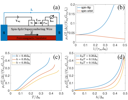
Figure 3: (a) Schematic view of the setup. Here the spin-splitting field is induced from either the ferromagnetic insulator or external magnetic field $\bf{B}$. (b-d) Spin accumulation as a function of parameters $\mu_{z}=\mu_{z}(h,T,\tau_{sn})$ at the detector position $L_{\rm det}=L/8$ in the linear response regime (small $V_{\rm inj}$). (b) The dependence on the spin relaxation rate for $k_{B}T=0.15\Delta_{0}$ and $h=0.3\Delta_{0}$. (c) Temperature and (d) spin-splitting field dependence. The orbital depairing rate is $\tau_{\rm orb}^{-1}=0.176h^{2}/\Delta_{0}$. Here we normalize the induced spin signal by the supercurrent amplitude $I_{s}$.

At first, we solve the kinetic equations using a perturbation expansion in the small parameter $\xi_{0}q_{s}$ where $\xi_{0}=\sqrt{D/\Delta}$ is the coherence length. For simplicity, we disregard inelastic scattering that would add an energy-non-local term in Eq. (6), and rather assume that $f_{L}=n_{0}$ at the ends of the wire. This mimics the typical experimental situation where the wire ends in wide electrodes, often at a distance small compared to the inelastic scattering length. In this case the solution of $f_{L}$ includes a linear component. The solution of $f_{T3}$, however, is determined by the strength of spin relaxation. This calculation is detailed in appendix C.

When $q_{s}=0$ we find $f_{T}$ and $f_{L3}$ modes generating the charge imbalance $\mu$. For $q_{s}\neq 0$ [see Eq. (7)] these solutions provide sources for the $f_{L}$ and $f_{T3}$ modes generating the spin accumulation $\mu_{z}$ in accordance with the qualitative mechanism illustrated in Fig. 1b. This generation takes place close to the injectors, before the charge imbalance relaxes due to the presence of an exchange field and depairing Bergeret et al. (2017); Hübler et al. (2010) (blue lines in Fig. 4a). However, $\mu_{z}$ has a long-range part associated with the contribution of $f_{L}$, which consists of two qualitatively different parts discussed below.

First, even in the absence of the supercurrent there exists a long-range contribution related to the already known heating effect Silaev et al. (2015) given by

$$f^{heat}_{L}(x)=\alpha_{heat}(|x|-L)$$ (14)

where $\alpha_{heat}=N_{+}n_{+}/D_{L}$. Besides that the long-range contribution excited due to the supercurrent is given approximatively by

$$f^{super}_{L}=\alpha_{super}({\rm sign}(x)-x/L)$$ (15)

The amplitude $\alpha_{super}$ depends on the strength of relaxation described by $R_{T/L3}$ and $S_{T3/L3}$ in Eq. (6).

Note that the spatial structures of (14) and (15) are different because $f^{heat}_{L}(x)$ is an even function and $f^{super}_{L}(x)$ is an odd function of $x$, see Fig. 4a. Besides that, the amplitude of supercurrent-induced part is an odd function of the injector voltage $\alpha_{super}(V_{inj})=-\alpha_{super}(-V_{inj})$. Therefore it exists already in the linear regime whereas the heating (14) is a nonlinear effect since $\alpha_{heat}(V_{inj})=\alpha_{heat}(-V_{inj})$. Besides that, as one can see from Eq. (14), the heating contribution grows linearly with the wire length $L$ while the supercurrent-related part (15) does not depend on the length $L$ at distances $|x|\ll L$.

To gain further insight, we first study the spin accumulation using a numerical solution of the kinetic equations. In Figs. 3b-d and  4a,b, we show the dependencies of the spin accumulation on various parameters $\mu_{z}=\mu_{z}(h,T,\tau_{sn},V_{\rm inj},x)$ obtained from the numerical solutions of Eqs. (6,7). Note that from this plot it is clear that the effect exists entirely due to the modification of quasiparticle spectrum by the spin splitting: As shown in Figs. 3c,d the spin signal $\mu_{z}$ disappears both for $h\to 0$ when there is no spin splitting and for $T\to 0$ when there are no quasiparticles. At the same time, Fig. 3b shows that the effect survives in the absence of spin-orbit or spin-flip scattering, i.e., for $\tau_{sn}\to\infty$. Below we study in more detail the influence of spin relaxation on the behaviour of different contributions to the spin accumulation.

IV.1 Case without spin relaxation ($S_{T3,L3}=0$)

The discussed mechanism of spin-charge conversion does not require any non-conservation of spin. This makes a qualitative distinction with previously discussed direct and inverse Edelstein effects which rely on the spin-orbit interaction.Edelstein (1995, 2003, 2005); Edel’shtein (1989); Houzet and Meyer (2015); Samokhin (2004); Dimitrova and Feigel’man (2007) In the absence of spin relaxation, $f_{T3}\propto x$ is also a long-range mode similar to the longitudinal one which in the absence of inelastic scattering is long-ranged, see Eqs. (14,15). The combination of $f_{T3}$ and $f_{L}$ then yields (see details in appendix C)

$$\mu_{z}=\xi_{0}\partial_{x}\varphi\frac{G_{\rm inj}}{G_{\xi_{0}}}\int_{0}^{\infty}d\epsilon n_{-}(\epsilon;V_{\rm inj})\sum_{\sigma=\uparrow,\downarrow}\frac{\sigma N_{\sigma}^{2}j_{s}^{\sigma}}{4D_{L}^{\sigma}R_{T}^{\sigma}}u_{0}(x).$$ (16)

Here $u_{0}(x)=-u_{0}(-x)$ is a function that decays linearly from unity close to the injector ($x=0$) to zero at the reservoirs and $n_{-}=[n_{0}(\epsilon+V_{\rm inj})-n_{0}(\epsilon-V_{\rm inj})]/2$. Equation (16) describes the region $|x|>\lambda_{cr}$, where $\lambda_{cr}$ is the charge relaxation length. Here $N_{\uparrow/\downarrow}$ are spin-up/down density of states, $D_{L}^{\uparrow/\downarrow}=D_{L}\pm D_{T3}$, $R_{T}^{\uparrow/\downarrow}=R_{T}\pm R_{L3}$, and $j_{s}^{\uparrow/\downarrow}=j_{E}\pm j_{Es}$. Moreover, $G_{\rm inj}$ and $G_{\xi_{0}}$ are the normal-state conductances of the injector and of a wire with length $\xi_{0}$, respectively. The integrand in Eq. (16) is peaked at $\epsilon\approx\Delta\pm h$ due to the BCS divergence in $N_{\sigma}$, $j_{s}^{\sigma}$ and $R_{T}^{\sigma}$. This divergence can be cut off by the depairing parameter Dynes et al. (1984) $\Gamma$ so that for $\epsilon=\Delta+\sigma h$, $N_{\sigma}\approx\gamma_{\sigma}^{-1/2}/\sqrt{2}$, $j_{S}^{\sigma}\approx\gamma_{\sigma}^{-1}/2$ and $R_{\sigma}\approx\gamma_{\sigma}^{-1/2}/2$ with $\gamma_{\sigma}=\Gamma/(\Delta+\sigma h)$. Therefore the integrand scales as $(8\gamma_{\sigma})^{-3/2}$, whereas the width of the peak is $\propto\Gamma$. Overall, this means a diverging integral scaling like $\sim\Gamma^{-1/2}$. Similar divergence was found in Ref. Schmid and Schön, 1979 for the supercurrent induced charge imbalance in the absence of spin splitting.

In practice, the relevant depairing mechanism in the presence of spin splitting and supercurrent is the orbital depairing due to the combined effect of the supercurrent itself and of an in-plane magnetic field $\mathbf{B}$ on the spectrum of the superconductor de Gennes (1999); Belzig et al. (1996); Anthore et al. (2003), with rate $\tau_{\rm orb}^{-1}=D\Delta(\partial_{x}\varphi)^{2}/(2)+De^{2}B^{2}d^{2}/6$ for a film with thickness $d$. It does not relax the spin, but affects the spectral properties of the superconductor by reshaping the singularities in the spectral quantities Bergeret et al. (2017). We can hence use $\tau_{\rm orb}^{-1}$ instead of $\Gamma$ to cut the divergence, and see that for very large phase gradients, $\mu_{z}$ becomes independent of $\partial_{x}\varphi$.

According to Eq. (16) the difference of the quantity $N_{0}^{2}j_{s}/(D_{L}R_{T})$ for spin up and down species describes the charge-spin conversion. We find that the charge imbalance is proportional to the energy integral of $N_{0}^{2}/R_{T}$, averaged over spin. The charge is then converted to spin at a rate $\propto j_{s}/D_{L}$. The temperature and exchange field dependence of $\mu_{z}$ are given in Figs. 3c and d, respectively. We can see that the linear-response $\mu_{z}\rightarrow 0$ as $T\rightarrow 0$, which reflects the freezing of the quasiparticle population (Fig. 3c). However, this can be circumvented by considering response at $V_{\rm inj}\sim\Delta$ as shown below. At the superconducting critical temperature $T_{c}$, the ratio $\mu_{z}/I_{s}$ diverges similarly to the supercurrent induced charge imbalance in the presence of a temperature gradient Clarke et al. (1979); Pethick and Smith (1980). Since $T_{c}$ is lower for a higher exchange field, this divergence happens at a lower temperature in a higher exchange field. For a fixed temperature, the divergence of $\mu_{z}$ also happens at a critical exchange field (Fig. 3d) where superconductivity is suppressed Chandrasekhar (1962); Clogston (1962).

IV.2 Effect of spin relaxation

Spin-flip and spin-orbit relaxation affect both spectral and nonquilibrium properties of the superconductor. For the spectral properties, spin-flip relaxation breaks the time-reversal symmetry and suppresses the superconducting pair potential and critical temperature, while spin-orbit scattering reduces the effect of the exchange field without suppressing the pair potential Bergeret et al. (2017). Both spin-flip and spin-orbit scattering also lead to the relaxation of $f_{T3}$ [terms $S_{T3/L3}$ in Eq. (6)]. For strong spin relaxation, the contribution to $\mu_{z}$ thus results only from $f_{L}$, and decays only via inelastic scattering. In this case (see details in appendix C)

$$\mu_{z}=\xi_{0}\partial_{x}\varphi_{0}\frac{G_{\rm inj}}{G_{\xi_{0}}}\int_{0}^{\infty}d\epsilon n_{-}(\epsilon;V_{\rm inj})\frac{\left(N_{\uparrow}^{2}-N_{\downarrow}^{2}\right)j_{E}}{4R_{T}D_{L}}u_{1}(x).$$ (17)

Here the linear function $u_{1}(x)=-u_{1}(-x)\approx u_{0}(x)$ for $|x|>\lambda_{cr}$. However, the effects of spin-flip/spin-orbit scattering on the spectral functions also affect the resulting $\mu_{z}$. The effect depends strongly on the type of scattering.

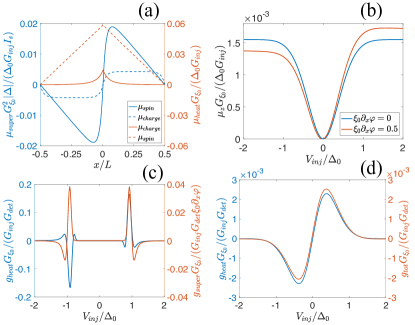
Figure 4: Spin accumulation and nonlocal conductance. (a) Position dependence of heat (red) and supercurrent (blue) induced charge and spin imbalances. Here the results are calculated for $T=0.15\Delta_{0}$, $h=0.3\Delta_{0}$ at $V_{\rm inj}=0.1\Delta_{0}$. The thick curves are odd and dashed curves are even in injection voltage. (b) Injection voltage dependence on spin accumulation for $T=0.25\Delta_{0}$. (c) Nonlocal conductance as a function of injection voltage in separate scales for heat and supercurrent induced effects (with $\xi_{0}\partial_{x}\varphi$=0.1) for $T=0.02\Delta_{0}$. (d) Heat induced and the total conductance as a function of injection voltage for $T=0.25\Delta_{0}$ (with $\xi_{0}\partial_{x}\varphi$=0.5). The parameters $\tau_{so}^{-1}=0.0475\Delta_{0}$, $\tau_{sf}^{-1}=0.0025\Delta_{0}$, $h=0.05\Delta_{0}$, and $L=20\xi_{0}$ are common in panels (b)-(d).

For pure spin-flip relaxation, contribution of $f_{L}$ increases as a function of the spin relaxation rate, and diverges when the strong relaxation completely kills superconductivity. This can be seen in the relaxation rate dependence of $\mu_{z}$ in the linear response regime in Fig. 3b. For pure spin-orbit relaxation, the effect of the exchange field is suppressed, and thereby also the charge-spin conversion.

V Spin accumulation and nonlocal conductance

The charge-spin conversion can be detected by inspecting the non-local conductance $g_{nl}=dI_{\rm det}/dV_{\rm inj}$ in the presence of the supercurrent $I_{s}$ driven across the wire. Without supercurrent, this quantity was measured in Refs.  Quay et al., 2013; Hübler et al., 2012; Wolf et al., 2013. We show an example of $g_{nl}$ in Fig. 4c-d. We separate it in different symmetry components vs. $V_{\rm inj}$ and $P_{\rm det}$ as

$$g_{nl}=g_{ee}+g_{eo}+(g_{oe}+g_{oo})P_{\rm det},$$ (18)

where $g_{\alpha e/o}(V_{\rm inj})=\pm g_{\alpha e/o}(-V_{\rm inj})$ and $\alpha=e/o$ describe the symmetry vs. $P_{\rm det}$. Since the derivative of the detector current with respect to $V_{\rm inj}$ flips the parity of the terms, the conductance due to the pure charge imbalance is even in both $V_{\rm inj}$ and $P_{\rm det}$ and hence is described by $g_{ee}$. The term $g_{oo}=g_{\rm heat}$ is the long-range spin accumulation due to the heat injection Silaev et al. (2015); Bobkova and Bobkov (2015). The supercurrent induces the term $g_{eo}$ that describes the conversion of temperature gradients to charge Schmid and Schön (1979); Pethick and Smith (1980); Clarke et al. (1979), whereas $g_{oe}=g_{\rm super}$ results from the supercurrent-induced charge-spin conversion. The symmetry of $g_{\rm super}$ results from the fact that it is related to spin imbalance (and therefore antisymmetric in $P_{\rm det}$) and originates from induced charge imbalance. In normal-metal spin injection experiments Jedema et al. (2001) only the term $g_{oe}$ is non-zero, but it requires non-zero spin polarization $P_{\rm inj}$ of the injector. Here $P_{\rm inj}=0$.

The term $g_{\rm super}$ should be compared to the contribution determined by effective heatingSilaev et al. (2015) (14)

$$g_{\rm heat}=\frac{G_{\rm inj}}{G_{\xi_{0}}}\frac{L}{2\xi_{0}}u_{3}(x)\int_{0}^{\infty}d\epsilon\frac{\partial n_{+}}{\partial V_{\rm inj}}\frac{N_{\uparrow}^{2}-N_{\downarrow}^{2}}{D_{L}},$$ (19)

where $u_{3}(x)=u_{3}(-x)$ is a linear function interpolating from unity at the injector to zero at the reservoirs and $n_{+}=(n_{0}(\epsilon+eV)+n_{0}(\epsilon-eV)-2n_{0})/2$. For $T\rightarrow 0$, $\partial n_{\pm}/\partial V_{\rm inj}$ approaches a $\delta$-function at $\epsilon=\pm eV$, and we can estimate the integrals by the values of the kinetic coefficients at those energies. For $eV\approx\Delta\pm h$ where the main signal resides, $g_{\rm super}\approx 2\xi_{0}g_{\rm heat}/L$ for $\xi_{0}\nabla\varphi\approx\tau_{\rm orb}^{-1}\Delta+\tau_{\rm sf}^{-1}+\tau_{\rm so}^{-1}$, i.e., when the supercurrent starts affecting the density of states. At higher temperatures and lower voltages $eV\lesssim k_{B}T$, where quasiparticle effects are visible even at linear response, $g_{\rm super}$ can dominate over $g_{\rm heat}$.

VI Conclusion

In conclusion, we have shown how the nonequilibrium supercurrent in a spin-split superconductor can partially convert charge imbalance to spin imbalance. The resulting spin imbalance is long-ranged, decaying only due to inelastic scattering. Here we have concentrated on a setup with collinear magnetizations. We expect that the generalization of our theory to the case with inhomogeneous magnetization would shed light on the possible coherently controllable nonequilibrium spin torques. We also expect to find analogous effects in superconducting proximity structures in the presence of spin splitting, i.e., combining the phenomena discussed in Refs. Virtanen and Heikkilä, 2004 and Machon et al., 2013.

Appendix A Self-consistency equation the for $\Delta$

The pair potential $\Delta$ should be obtained self-consistently from

$$\Delta=\frac{\lambda}{16}\int_{-\Omega_{D}}^{\Omega_{D}}d\epsilon\operatorname{Tr}\bigg{[}(\tau_{1}-i\tau_{2})\hat{g}^{K}(\epsilon)\bigg{]},$$ (20)

where $\lambda$ is the coupling constant and $\Omega_{D}$ is the Debye cutoff energy. In the presence of both spin splitting and non-equilibrium distribution functions, this goes to the form Bergeret et al. (2017)

$$\begin{split}\Delta=&\frac{\lambda}{2}\int_{-\Omega_{D}}^{\Omega_{D}}d\varepsilon\left[{\rm Im}g_{01}^{R}f_{L}+{\rm Im}g_{31}^{R}f_{T3}\right.\\ &\left.+i({\rm Re}g_{01}^{R}f_{T}+{\rm Re}g_{31}^{R}f_{L3})\right],\end{split}$$ (21)

where $g_{ij}^{R}$ is the part of the Retarded Green’s function proportional to $\sigma_{i}\tau_{j}$. The results obtained in the main text use the self-consistent equilibrium gap, but do not include the nonequilibrium corrections. For the gap amplitude $|\Delta|$ this approximation is justified in the case of low injection conductance $G_{\rm inj}$. However, with such a choice the charge current is strictly speaking not conserved in the presence of a constant phase gradient. This is because the quasiparticle injection modifies the phase of $\Delta$ (the two last terms in Eq. (21)), and the true phase gradient corresponding to a constant charge current becomes position dependent. Such an effect is of a higher order in the phase gradient, and within a perturbation approach can therefore be disregarded. We leave such higher-order effects for further work.

Appendix B Kinetic coefficients

The Green’s function in Eq. (2) satisfies the normalization condition $\check{g}^{2}=1$, which allows us to parameterize the Keldysh Green’s function as $\check{g}^{K}=\check{g}^{R}\check{f}-\check{f}\check{g}^{A}$, where the distribution matrix $\check{f}=f_{L}+f_{T}\tau_{3}+f_{T3}\sigma_{3}+f_{L3}\sigma_{3}\tau_{3}$. We also can parameterize the retarded Green’s function as $\check{g}^{R}=g_{01}\tau_{1}+g_{02}\tau_{2}+g_{03}\tau_{3}+g_{31}\sigma_{3}\tau_{1}+g_{32}\sigma_{3}\tau_{2}+g_{33}\sigma_{3}\tau_{3}$, and $\check{g}^{A}=-\tau_{3}\check{g}^{R\dagger}\tau_{3}$. Here $g_{i}$ are complex scalar functions. From these, we identify $N_{+}=\text{Re}(g_{03})$ and $N_{-}=\text{Re}(g_{33})$.

The kinetic coefficients $D_{i}$, $R_{i}$, and $S_{i}$ in Eq. (3) and Eq. (4) can be expressed in terms of the parameterized functions $\check{g}^{R}$ and $\check{g}^{A}$. The $D_{i}$s are

$$\begin{split}D_{L}=&\frac{D}{2}(1-|g_{01}|^{2}-|g_{02}|^{2}+|g_{03}|^{2}-|g_{31}|^{2}\\ &-|g_{32}|^{2}+|g_{33}|^{2})\end{split}$$

$$\begin{split}D_{T3}=&-D\left[\text{Re}(g_{01}g_{31}^{*})+\text{Re}(g_{02}g_{32}^{*})-\text{Re}(g_{03}g_{33}^{*})\right]\end{split}$$

$$\begin{split}D_{T}=&\frac{D}{2}(1+|g_{01}|^{2}+|g_{02}|^{2}+|g_{03}|^{2}+|g_{31}|^{2}\\ &+|g_{32}|^{2}+|g_{33}|^{2})\end{split}$$

$$\begin{split}D_{L3}=&D\left[\text{Re}(g_{01}g_{31}^{*})+\text{Re}(g_{02}g_{32}^{*})+\text{Re}(g_{03}g_{33}^{*})\right].\end{split}$$

The $R_{i}$s are

$$R_{T} =\text{Re}(g_{01})\Delta\cos\varphi-\text{Re}(g_{02})\Delta\sin\varphi$$

$$R_{L3} =\text{Re}(g_{31})\Delta\cos\varphi-\text{Re}(g_{32})\Delta\sin\varphi.$$

The $S_{i}$s are

$$\begin{split}S_{L3}&=\tau_{sn}^{-1}\left\{\text{Re}(g_{03})^{2}-\text{Re}(g_{33})^{2}\right.\\ &\left.+\beta\left[\text{Im}(g_{01})^{2}-\text{Im}(g_{31})^{2}+\text{Im}(g_{02})^{2}-\text{Im}(g_{32})^{2}\right]\right\}\end{split}$$

$$\begin{split}S_{T3}&=\tau_{sn}^{-1}\left\{\text{Re}(g_{03})^{2}-\text{Re}(g_{33})^{2}\right.\\ &\left.+\beta\left[\text{Re}(g_{31})^{2}-\text{Re}(g_{01})^{2}+\text{Re}(g_{32})^{2}-\text{Re}(g_{02})^{2}\right]\right\},\end{split}$$

where $\tau_{sn}^{-1}=\tau_{so}^{-1}+\tau_{sf}^{-1}$ and the parameter $\beta=(\tau_{so}-\tau_{sf})/(\tau_{so}+\tau_{sf})$ describes the relative strength of the spin-orbit and spin-flip scattering. For $\beta>0$, spin-flip scattering dominates the spin-orbit scattering, and vice versa for $\beta<0$. These coefficients are independent of $\varphi$ (the dependence of $\varphi$ in $R_{i}$ terms is canceled by the corresponding terms in $g_{i}$).

There are also two more coefficients in Eq. (3) and Eq. (4), spectral supercurrent and spectral spin supercurrent, which depend on the phase gradient $\partial_{x}\varphi$

$$j_{E}\partial_{x}\varphi =\frac{1}{8}D\operatorname{Tr}\left[\left(\check{g}^{R}\partial_{x}\check{g}^{R}-\check{g}^{A}\partial_{x}\check{g}^{A}\right)\tau_{3}\right]$$

$$j_{Es}\partial_{x}\varphi =\frac{1}{8}D\operatorname{Tr}\left[\left(\check{g}^{R}\partial_{x}\check{g}^{R}-\check{g}^{A}\partial_{x}\check{g}^{A}\right)\sigma_{3}\tau_{3}\right].$$

These two terms are related to the nonzero charge supercurrrent and spin-energy current. Here and below we assume that the wire is in the $x$ direction and all changes in the phase $\varphi$ and the distribution functions take place in that direction.

Appendix C Perturbation theory solutions of kinetic equations in the linear order by $\xi_{0}\nabla\varphi$.

The general solution of the kinetic equations in Eq. (3) can be written as

$$\begin{pmatrix}f_{L},&f_{T3},&f_{T},&f_{L3}\end{pmatrix}^{T}=(C_{01}+C_{02}x)\textbf{v}_{0}^{T}+C_{1}e^{k_{L}x}\textbf{v}_{1}^{T}+C_{2}e^{-k_{L}x}\textbf{v}_{2}^{T}+C_{3}e^{k_{T1}x}\textbf{v}_{3}^{T}+C_{4}e^{-k_{T1}x}\textbf{v}_{4}^{T}+C_{5}e^{k_{T2}x}\textbf{v}_{5}^{T}+C_{6}e^{-k_{T2}x}\textbf{v}_{6}^{T},$$ (22)

where $\textbf{v}_{0}^{T}=(1,0,0,0)^{T}$, $k_{L}$, $k_{T1}$ and $k_{T2}$ are the energy dependent inverse length scales, the other $\textbf{v}_{i}^{T}$s can be determined numerically, and $C_{i}$s can be determined from the boundary conditions (10). For a small phase gradient, we can determine these coefficients analytically. Below we concentrate in particular on the solutions of the modes related to the supercurrent induced spin imbalance and treat the supercurrent as a perturbation in the kinetic equations. In the zeroth order Eq. (3) decouples into two sets of kinetic equations. First we concentrate on the part odd in the injection voltage, describing charge imbalance. In this case, for a vanishing supercurrent the relevant distribution function components are $f_{T}$ and $f_{L3}$. We denote their values in the absence of supercurrent by $f_{T}^{0}$ and $f_{L3}^{0}$. On the other hand, the supercurrent couples them to the other two functions $f_{L}$ and $f_{T3}$ and induces the change $\delta f_{L}$ and $\delta f_{T3}$ which we calculate to linear order in the phase gradient. For $f_{T}$ and $f_{L3}$, we get the first set of kinetic equations

$$\begin{pmatrix}D_{T}&D_{L3}\\ D_{L3}&D_{T}\end{pmatrix}\begin{pmatrix}\partial_{x}^{2}f_{T}^{0}\\ \partial_{x}^{2}f_{L3}^{0}\end{pmatrix}=\begin{pmatrix}R_{T}&R_{L3}\\ R_{L3}&R_{T}+S_{L3}\end{pmatrix}\begin{pmatrix}f_{T}^{0}\\ f_{L3}^{0}\end{pmatrix}.$$ (23)

In what follows, we choose $\Delta_{0}$ as the reference energy scale, and therefore the coherence length $\xi_{0}=\sqrt{\hbar D/\Delta_{0}}$ becomes the reference length scale. That means, for example, that the dimensionless quantities describing spin relaxation are of the form $\tau_{\rm sf}\Delta_{0}$ and $\tau_{\rm so}\Delta_{0}$.

Using the boundary conditions (10), we obtain for $\kappa_{I}L\ll 1$

$$\begin{pmatrix}f_{T}^{0}\\ f_{L3}^{0}\end{pmatrix}=\kappa_{I}\xi_{0}n_{-}(\epsilon,V_{inj})\sum_{i=1,2}A_{i}e^{-k_{Ti}x/\xi_{0}}\begin{pmatrix}k_{R_{i}}\\ -1\end{pmatrix},\ 0\leq x\leq\frac{L}{2}$$ (24)

where the inverse length scales

$$k_{T1/2}^{2}=\frac{D_{T}(2R_{T}-S_{L3})-2D_{L3}R_{L3}{\pm}\sqrt{4(D_{T}R_{L3}-D_{L3}R_{T})^{2}+4D_{L3}(-D_{T}R_{L3}+D_{L3}R_{T})S_{L3}+D_{T}^{2}S_{L3}^{2}}}{2(D_{T}^{2}-D_{L3}^{2})},$$

and the coefficients

$$A_{i}=\frac{\left[N_{-}(D_{L3}-D_{T}k_{Ri^{\prime}})-N_{+}(D_{T}-D_{L3}k_{Ri^{\prime}})\right]}{4(D_{L3}^{2}-D_{T}^{2})(k_{Ri}-k_{Ri^{\prime}})k_{Ti}},$$

$$k_{R1/2}=\frac{D_{T}S_{L3}{\mp}\sqrt{4D_{L3}^{2}R_{T}(R_{T}+S_{L3})-4D_{L3}D_{T}R_{L3}(2R_{T}+S_{L3})+D_{T}^{2}(4R_{L3}^{2}+S_{L3}^{2})}}{2(D_{T}R_{L3}-D_{L3}R_{T})}.$$

For the perturbed terms of $f_{L}$ and $f_{T3}$, we get another set of kinetic equations

$$\begin{pmatrix}D_{L}&D_{T3}\\ D_{T3}&D_{L}\end{pmatrix}\begin{pmatrix}\partial_{x}^{2}\delta f_{L}\\ \partial_{x}^{2}\delta f_{T3}\end{pmatrix}+\begin{pmatrix}j_{E}\partial_{x}\varphi&j_{Es}\partial_{x}\varphi\\ j_{Es}\partial_{x}\varphi&j_{E}\partial_{x}\varphi\end{pmatrix}\begin{pmatrix}\partial_{x}f_{T}^{0}\\ \partial_{x}f_{L3}^{0}\end{pmatrix}=\begin{pmatrix}0&0\\ 0&S_{T3}\end{pmatrix}\begin{pmatrix}\partial_{x}^{2}\delta f_{L}\\ \partial_{x}^{2}\delta f_{T3}\end{pmatrix}.$$ (25)

Using the solution in Eq. (24), we obtain

$$\begin{pmatrix}\delta f_{L}\\ \delta f_{T3}\end{pmatrix}=\kappa_{I}\xi_{0}^{2}\partial_{x}\varphi n_{-}(\epsilon,V_{inj})\sum_{i=1,2}\left[\frac{\alpha_{i}}{k_{L}^{2}-k_{Ti}^{2}}(e^{-k_{Ti}x/\xi_{0}}-e^{-k_{L}x/\xi_{0}})\begin{pmatrix}-D_{T3}/D_{L}\\ 1\end{pmatrix}\right.$$

$$\left.+\frac{\beta_{i}}{k_{Ti}^{2}}\left(\frac{2x}{L}-1+e^{-k_{Ti}x/\xi_{0}}\right)\left(\begin{array}[]{c}1\\ 0\end{array}\right)\right],\ 0\leq x\leq\frac{L}{2},$$ (26)

where the inverse length scale

$$k_{L}^{2}=\frac{S_{T3}D_{L}}{D_{L}^{2}-D_{T3}^{2}},$$

and the coefficients

$$\alpha_{i}=\frac{[j_{Es}(D_{T3}+D_{L}k_{Ri})-j_{E}(D_{L}+D_{T3}k_{Ri})][N_{-}(D_{L3}-D_{T}k_{Ri^{\prime}})-N_{+}(D_{T}-D_{L3}k_{Ri^{\prime}})]}{2(D_{T}^{2}-D_{L3}^{2})(D_{L}^{2}-D_{T3}^{2})(k_{Ri}-k_{Ri^{\prime}})},$$

$$\beta_{i}=\frac{(j_{E}k_{Ri}-j_{Es})[N_{+}(D_{T}-D_{L3}k_{Ri^{\prime}})-N_{-}(D_{L3}-D_{T}k_{Ri^{\prime}})]}{2D_{L}(D_{T}^{2}-D_{L3}^{2})(k_{Ri}-k_{Ri^{\prime}})}.$$

The spin accumulation generated from the supercurrent is

$$\mu_{z}=\frac{1}{2}\int_{0}^{\infty}d\epsilon(N_{+}\delta f_{T3}+N_{-}\delta f_{L})$$

$$=\frac{1}{2}\kappa_{I}\xi_{0}^{2}\partial_{x}\varphi\int_{0}^{\infty}d\epsilon\ n_{-}(\epsilon,V_{inj})\sum_{i=1,2}\left[\left(N_{+}-N_{-}\frac{D_{T3}}{D_{L}}\right)\frac{\alpha_{i}}{k_{L}^{2}-k_{Ti}^{2}}(e^{-k_{Ti}x/\xi_{0}}-e^{-k_{L}x/\xi_{0}})\right.$$

$$\left.+N_{-}\frac{\beta_{i}}{k_{Ti}^{2}}\left(\frac{2x}{L}-1+e^{-k_{Ti}x/\xi_{0}}\right)\right],\ 0\leq x\leq\frac{L}{2}.$$ (27)

In the extreme limit of $\tau_{sn}^{-1}\rightarrow 0$, this result can be reduced to a simpler form. In this case, $S_{T3}$ and $S_{L3}$ terms in the kinetic equations are zero, therefore, $e^{-k_{L}x/\xi_{0}}$ term is replaced by a linear term with same coefficients with $\delta f_{L}$. For the linear response regime $n_{-}(\epsilon,V_{inj})=V_{inj}\partial n_{0}/\partial\epsilon$, we get

$$\mu_{z}=V_{inj}\kappa_{I}\xi_{0}^{2}\partial_{x}\varphi\int_{0}^{\infty}d\epsilon\frac{\partial n_{0}}{\partial\epsilon}\left[\frac{N_{\uparrow}^{2}j_{s}^{\uparrow}}{4D_{L}^{\uparrow}R_{T}^{\uparrow}}\left(\frac{2x}{L}-1+e^{-\sqrt{R_{T}^{\uparrow}/D_{T}^{\uparrow}}x/\xi_{0}}\right)\right.$$

$$\left.-\frac{N_{\downarrow}^{2}j_{s}^{\downarrow}}{4D_{L}^{\downarrow}R_{T}^{\downarrow}}\left(\frac{2x}{L}-1+e^{-\sqrt{R_{T}^{\downarrow}/D_{T}^{\downarrow}}x/\xi_{0}}\right)\right],\ 0\leq x\leq\frac{L}{2},$$ (28)

where the $\uparrow$ and $\downarrow$ quantities are the addition and subtraction of the singlet and triplet components of the spectral quantities, $j_{s}^{\uparrow/\downarrow}=j_{E}\pm j_{Es}$, $N_{\uparrow/\downarrow}=N_{+}\pm N_{-}$, $D_{L}^{\uparrow/\downarrow}=D_{L}\pm D_{T3}$, and $R_{\uparrow/\downarrow}=R_{T}\pm R_{L3}$.

It is straightforward to see that $\mu_{z}=0$ for $h=0$, since the quantity $N^{2}j_{s}/(D_{L}R_{T})$ is equal for both spin species. For nonzero $h$ the difference of this quantity for different spin species gives the spin accumulation. However, without relaxation, this quantity is proportional to $1/\sqrt{\Gamma}$, which describes the broadening of the spectral quantities.

In practice, the relevant broadening renormalizing $\mu_{z}$ comes from the orbital effect due to either a magnetic field or the phase gradient itself de Gennes (1999); Belzig et al. (1996); Anthore et al. (2003), or due to terms contributing to the spin relaxation Bergeret et al. (2017). The two first effects can be described by an orbital relaxation rate $\tau_{\rm orb}^{-1}=(\xi_{0}\partial_{x}\varphi)^{2}/2+(De^{2}B^{2}d^{2}/6)$ Anthore et al. (2003), where $B$ is the magnetic field, and $d$ is the film thickness. In the presence of spin relaxation described by the rate $\tau_{\rm sn}^{-1}$, an estimate for the overall broadening comes from $\Gamma\mapsto\tau_{\rm orb}^{-1}+\tau_{\rm sn}^{-1}$, but the exact amount depends on the relaxation mechanism and the size of the exchange field. As an example, we show the supercurrent induced $\mu_{z}$ vs. $\tau_{\rm orb}^{-1}$ in Fig. 5(a). Since $\mu_{z}\propto(\xi_{0}\partial_{x}\varphi)\Gamma^{-1/2}$, for large phase gradients satisfying $\xi_{0}\partial_{x}\varphi\gg\sqrt{De^{2}B^{2}d^{2}/6}+\tau_{sn}^{-1}$, the spin accumulation becomes independent of $\partial_{x}\varphi$.

$\begin{array}[]{c}\includegraphics[width=433.62pt]{figure5}\end{array}$

Figure 5: Spin accumulation with and without relaxation in the linear response regime. (a) The dependence on orbital depairing rate in the case without spin relaxation. Position dependence in the case of pure spin-flip relaxation (b) and pure spin-orbit relaxation (c). An exchange field $h=0.3\Delta_{0}$ is common for all panels, and a temperature $T=0.15\Delta_{0}$ is used in (b) and (c) panels. The red curves describe the charge imbalance. The spin relaxation length is defined as $\lambda_{sn}=\sqrt{\tau_{sn}D}$.

However, spin relaxation affects also the decay of the nonequilbrium components of the distrubution function via the relaxation terms $\sim S_{T/L3}$. In another extreme limit $\tau_{sn}\rightarrow\infty$, we also can have a simpler form of Eq. (28). In this case $4D_{L3}(D_{T}R_{L3}-D_{L3}R_{T})/D_{T}^{2}\ll S_{L3}$, and

$$\mu_{z}=V_{inj}\kappa_{I}\xi_{0}^{2}\partial_{x}\varphi\int_{0}^{\infty}d\epsilon\frac{\partial n_{0}}{\partial\epsilon}\frac{\left(N_{\uparrow}^{2}-N_{\downarrow}^{2}\right)j_{E}}{4R_{T}D_{L}}\left(\frac{2x}{L}-1+2e^{-k_{T2}x/\xi_{0}}-e^{-k_{L}x/\xi_{0}}\right),\ 0\leq x\leq\frac{L}{2}.$$ (29)

Here, except the density of states, the triplet component of other spectral quantities do not contribute to the spin accumulation. The difference of the density of states for two spin species behaves differently for spin-orbit and spin-flip relaxations. Spin-orbit relaxation does not affect the pair potential but tries to lift the effect of the spin-splitting field. Therefore, $\mu_{z}$ approaches zero for very strong relaxation (S4(c)). In the case of spin-flip relaxation, it suppresses the pair potential, therefore, spin-accumulation diverges the strong spin-flip relaxations destroys the superconductivity (S4(b)).

References

- Tinkham (1996) M. Tinkham, Introduction to superconductivity (Courier Corporation, 1996).
- Schmid and Schön (1975) A. Schmid and G. Schön, J. Low Temp. Phys. 20, 207 (1975).
- Bergeret et al. (2017) F. S. Bergeret, M. Silaev, P. Virtanen, and T. T. Heikkilä, arXiv preprint arXiv:1706.08245 (2017).
- Silaev et al. (2015) M. Silaev, P. Virtanen, F. Bergeret, and T. T. Heikkilä, Phys. Rev. Lett. 114, 167002 (2015).
- Bobkova and Bobkov (2015) I. V. Bobkova and A. M. Bobkov, JETP Lett. 101, 118 (2015).
- Schmid and Schön (1979) A. Schmid and G. Schön, Phys. Rev. Lett. 43, 793 (1979).
- Clarke et al. (1979) J. Clarke, B. Fjordbøge, and P. Lindelof, Phys. Rev. Lett. 43, 642 (1979).
- Pethick and Smith (1980) C. Pethick and H. Smith, J. Phys. C: Solid State Phys. 13, 6313 (1980).
- Pethick and Smith (1979) C. J. Pethick and H. Smith, Phys. Rev. Lett. 43, 640 (1979).
- Edelstein (1995) V. M. Edelstein, Phys. Rev. Lett. 75, 2004 (1995).
- Edelstein (2003) V. M. Edelstein, Phys. Rev. B 67, 020505 (2003).
- Edelstein (2005) V. M. Edelstein, Phys. Rev. B 72, 172501 (2005).
- Edel’shtein (1989) V. Edel’shtein, Sov. Phys. JETP 68, 1244 (1989).
- Houzet and Meyer (2015) M. Houzet and J. S. Meyer, Phys. Rev. B 92, 014509 (2015).
- Samokhin (2004) K. V. Samokhin, Phys. Rev. B 70, 104521 (2004).
- Dimitrova and Feigel’man (2007) O. Dimitrova and M. V. Feigel’man, Phys. Rev. B 76, 014522 (2007).
- Buzdin (2008) A. Buzdin, Phys. Rev. Lett. 101, 107005 (2008).
- Konschelle et al. (2015) F. Konschelle, I. V. Tokatly, and F. S. Bergeret, Phys. Rev. B 92, 125443 (2015).
- Bobkova et al. (2016) I. V. Bobkova, A. M. Bobkov, A. A. Zyuzin, and M. Alidoust, Phys. Rev. B 94, 134506 (2016).
- Bobkova and Bobkov (2017) I. V. Bobkova and A. M. Bobkov, Phys. Rev. B 95, 184518 (2017).
- Szombati et al. (2016) D. B. Szombati, S. Nadj-Perge, D. Car, S. R. Plissard, E. P. A. M. Bakkers, and L. P. Kouwenhoven, Nature Physics 12, 568 EP (2016).
- Assouline et al. (2018) A. Assouline, C. Feuillet-Palma, N. Bergeal, T. Zhang, A. Mottaghizadeh, A. Zimmers, E. Lhuillier, M. Marangolo, M. Eddrief, P. Atkinson, M. Aprili, and H. Aubin, “Spin-orbit induced phase-shift in bi2se3 josephson junctions,” (2018), arXiv:1806.01406 .
- Murani et al. (2017) A. Murani, A. Kasumov, S. Sengupta, Y. A. Kasumov, V. T. Volkov, I. I. Khodos, F. Brisset, R. Delagrange, A. Chepelianskii, R. Deblock, H. Bouchiat, and S. Guéron, Nature Communications 8, 15941 (2017).
- Kato et al. (2004) Y. K. Kato, R. C. Myers, A. C. Gossard, and D. D. Awschalom, Phys. Rev. Lett. 93, 176601 (2004).
- Quay et al. (2013) C. Quay, D. Chevallier, C. Bena, and M. Aprili, Nature Physics 9, 84 (2013).
- Hübler et al. (2012) F. Hübler, M. J. Wolf, D. Beckmann, and H. v. Löhneysen, Phys. Rev. Lett. 109, 207001 (2012).
- Wolf et al. (2013) M. J. Wolf, F. Hübler, S. Kolenda, H. v. Löhneysen, and D. Beckmann, Phys. Rev. B 87, 024517 (2013).
- Bergeret et al. (2005) F. Bergeret, A. Volkov, and K. Efetov, Rev. Mod. Phys. 77, 1321 (2005).
- Heikkilä et al. (2002) T. T. Heikkilä, J. Särkkä, and F. K. Wilhelm, Phys. Rev. B 66, 184513 (2002).
- Kuprianov and Lukichev (1988) M. Y. Kuprianov and V. Lukichev, Zh. Eksp. Teor. Fiz 94, 149 (1988).
- Bergeret et al. (2012) F. Bergeret, A. Verso, and A. F. Volkov, Phys. Rev. B 86, 214516 (2012).
- Tinkham and Clarke (1972) M. Tinkham and J. Clarke, Phys. Rev. Lett. 28, 1366 (1972).
- Hübler et al. (2010) F. Hübler, J. C. Lemyre, D. Beckmann, and H. v. Löhneysen, Phys. Rev. B 81, 184524 (2010).
- Dynes et al. (1984) R. C. Dynes, J. P. Garno, G. B. Hertel, and T. P. Orlando, Phys. Rev. Lett. 53, 2437 (1984).
- de Gennes (1999) P. G. de Gennes, Superconductivity of Metals and Alloys, Advanced book classics (Perseus, Cambridge, MA, 1999).
- Belzig et al. (1996) W. Belzig, C. Bruder, and G. Schön, Phys. Rev. B 54, 9443 (1996).
- Anthore et al. (2003) A. Anthore, H. Pothier, and D. Esteve, Phys. Rev. Lett. 90, 127001 (2003).
- Chandrasekhar (1962) B. S. Chandrasekhar, Appl. Phys. Lett. 1, 7 (1962).
- Clogston (1962) A. M. Clogston, Phys. Rev. Lett. 9, 266 (1962).
- Jedema et al. (2001) F. J. Jedema, A. Filip, and B. Van Wees, Nature 410, 345 (2001).
- Virtanen and Heikkilä (2004) P. Virtanen and T. T. Heikkilä, Phys. Rev. Lett. 92, 177004 (2004).
- Machon et al. (2013) P. Machon, M. Eschrig, and W. Belzig, Phys. Rev. Lett. 110, 047002 (2013).