USING FLOW MODELS WITH SENSITIVITIES TO STUDY COST EFFICIENT MONITORING PROGRAMS OF CO₂ STORAGE SITES

Abstract.

A key part of planning CO2 storage sites is to devise a monitoring strategy. The aim of this strategy is to fulfill the requirements of legislations and lower cost of the operation by avoiding operational problems. If CCS is going to be a widespread technology to deliver energy without CO2 emissions, cost-efficient monitoring programs will be a key to reduce the storage costs. A simulation framework, previously used to estimate flow parameters at Sleipner Layer 9 [1], is here extended and employed to identify how the number of measurements can be reduced without significantly reducing the obtained information. The main part of the methodology is based on well-proven, stable and robust, simulation technology together with adjoint-based sensitivities and data mining techniques using singular value decomposition (SVD). In particular we combine the simulation framework with time-dependent (seismic) measurements of the migrating plume. We also study how uplift data and gravitational data give complementary information.

We apply this methodology to the Sleipner project, which provides the most extensive data for CO2 storage to date. Since injection commenced in 1996, a series of seismic images have been taken to capture the migrating CO2 plume. First, we obtain a direct match with current measurements by calibrating topography, permeability, CO2 density, porosity, and injection rates. Using an estimate of the misfit, we show how one can minimize the number of measurements without significantly influencing the accuracy of the parameter estimates. We also investigate how assumptions on measurement errors influence the parameter estimate uncertainties.

The original benchmark model of Sleipner Layer 9 assumed a CO2 density of 760 kg/m3 and a significantly lower permeability than what we obtain from the above estimate. Using this as the assumed physical situation we show how the measurement sensitivities depend on the main dynamics of the systems. In particular we show that the sensitivity to the topography near the injection point is significantly less than for the matched case.

We also study the effect of measurement sparsity in space and time and show that for the current description of Layer 9, a limited number of measurements of the CO2-Water contact is sufficient to estimate the main dynamics The results are robust with respect to the choice of measurement points, despite the fact that the dynamics is sensitive to small changes in the top-surface topography at particular points, which is identified as spill points. By using a singular value decomposition (SVD), we show that the response of a small change in topography at the spill points gives global effect for this physical situation.

Finally, we extend the modelling framework with possibilities to incorporate gravity data based on gravitational changes. Using the sensitivities, we discuss in which situation different measurements can be utilized to give new information about the physical model.

For this study we utilize a vertical-equilibrium (VE) flow model for computational efficiency as implemented in the open-source software MRST-co2lab. However, our methodology for deriving efficient monitoring schemes is not restricted to VE-type flow models, and at the end, we discuss how the methodology can be used in the context of full 3D simulations.

1. Introduction

The Norwegian Continental Shelf offers enormous volumes of potential storage capacity for CO₂ in saline aquifers [1]. To enable large-scale CO₂ storage, prospective operators need effective monitoring strategies for detecting potential leakages and other undesired effects such as uplift and subsidence. This will require monitoring technologies, whose raw observation data should be assimilated into forecast models to confirm that the CO₂ plume is behaving as expected and provide support for decision making and remediation planning in the case of unpredicted events. We believe that the starting point for designing combined monitoring–forecast strategies should be simple robust reservoir models and inversion strategies localized as much as possible near the storage aquifer. Depth-integrated flow models that rely on an assumption of vertical equilibrium have been shown to work well for aquifers with good-quality sand, which is the most likely candidates for storage. In this work, we will use this as our reservoir model. The most used measurement for inversion is based on seismics. Traditionally seismic is used to estimate the static properties of the full formation, but with time-lapse seismic changes can be estimated. Most processing methods need a detailed model of the overburden. However Marchenko imaging have newly been applied to real field data [2] and only need limited information of the overburen. A second step, which often makes combining flow modeling and inversion methods difficult is that the estimated quantities do not coincide with the model parameters used in forward simulation. To bridge this gap it is essential introduce model of how changes in pressure and fluid saturations and compositions affect the seismic responses to be able to invert time-lapse seismic to update petrophysical properties of the geological model [3, 4]. We will not consider detailed inversion models for seismic but assume that plume heights can be estimated. In addition, we will use direct gravity changes as a second observation.

Traditionally, inversion is utilized to constrain the aquifer modeling. That is, you acquire time-lapse data by example seismic, gravity or electro magnetic techniques and these data can be inverted to determine changes in reservoir properties. Then, parameters in the reservoir model are changed to minimize the misfit between observed and simulated responses. However, it is also possible to use the flow model to constrain the seismic inversion so that the form of the inverted interfaces can be explained by the flow physics. In fact this is the simples way of ensuring the saturation and pressure changes has the right physical behavior. Likewise, one can use the flow model to investigate the measurability of model parameters, determine the optimal design of measurements and assess the effect of acquiring new measurements (value of information).

To illustrate we use the benchmark model of of the sleipner injection [5]. In a previous paper [6] we used a simulation model based on vertical-equilibrium to match to the real estimated plume shape [7, 8]. We use this work as a starting point to investigate how the sensitivity of the model changes with regard to the physical situation. To demonstrate this we use the original benchmark model and a member of the family of matched models. We investigate in detail how these models have different response in terms of measured quantities like plume-shape and gravity field. In particular, we show that combinations of gravity data and total mass injected is sufficient to determine the global parameters. The plume data however give more information about the top surface in particular for the physical situation of the match data.

Starting from this, we investigate the most important data in the setting of optimal design of experiment. Rather than a full investigation in terms of the actual measurements we calculate the optimal design with respect to the estimate of the plume heights and the gravity changes. This will give a starting point for evaluating cost-efficient monitoring strategies. To this end, we investigate different formulation of optimal design algorithms which can be extended to a more detailed analysis of the best monitoring strategy. We discuss the importance of having accurate estimates of correlations both in time and space of the estimated quantities to be able to make accurate estimates of the model and to evaluate the best monitoring strategy.

2. Methods

2.1. Governing equations – Darcy-based approach

The basic mechanisms of CO₂ injection and migration can be modeled using two components, water ($w$) and CO₂ ($g$), which at aquifer conditions will appear in an aqueous and a supercritical (liquid) phase, respectively. The flow dynamics is described by mass conservation,

(1) $$\frac{\partial(\phi\rho_{\alpha}s_{\alpha})}{\partial t}+\nabla\cdot\rho_{\alpha}\textbf{u}_{\alpha}=\rho_{\alpha}q_{\alpha},\quad\quad\alpha=w,g,$$

where $\phi$ is the porosity, $s_{\alpha}$ is the fluid saturation, $\rho_{\alpha}$ the fluid density, $\textbf{u}_{\alpha}$ the fluid velocity, $q_{\alpha}$ the volumetric flux caused by any source or sink, and $\alpha$ denotes the fluid phase. The fluid velocity is given by Darcy’s equation,

(2) $$\textbf{u}_{\alpha}=-k\lambda_{\alpha}(\nabla p_{\alpha}-\rho_{\alpha}\textbf{g}),$$

where $k$ is the absolute rock permeability; $\lambda_{\alpha}=k_{r\alpha}/\mu_{\alpha}$ is the fluid mobility, where $k_{r\alpha}=k_{r\alpha}(s_{w})$ and $\mu_{\alpha}$ denote the relative permeability and fluid viscosity, respectively; $p_{\alpha}$ is the pressure; and g is gravitational acceleration. The sum of the saturations are equal to unity, and fluid mobilities and capillary pressure ($p_{c}$) are expressed as functions of water saturation,

(3) $$s_{w}+s_{g}=1,$$

(4) $$\lambda_{\alpha}=\lambda_{\alpha}(s_{w}),$$

(5) $$p_{c}=p_{n}-p_{w}=P_{c}(s_{w}).$$

In [6] we demonstrated that for this equation with regard to plume shape there exist one exact invariant with respect to plume shape given by

(6) $$\phi=c\bar{\phi},\quad k=c\bar{k},\quad q_{\alpha}=c\bar{q}_{\alpha},$$

where $c$ is a positive constan.,In addition, there will be an approximate invariant given by $\delta\rho K=(\rho_{w}-\rho K)$ a constant.

If we, however extend to gravity response

(7) $$\Delta\textbf{g}(\textbf{r})=\int\frac{(\textbf{r}-\textbf{x})}{|\textbf{r}-\textbf{x}|^{3}}(\rho_{w}-\rho_{co_{2}})\,s\,\phi\mathrm{d}x^{3}$$

we can no longer change the product of $\Delta\rho\phi$ without changing the response.

The actual calculations presented in this paper will be done using the vertical equilibrium model also used in [6]. For a more detailed descriptions see [9].

2.2. Adjoint based gradients

In this section we consider matching uncertain topography and model parameters to observed responses through the use of simulation-based optimization. Let $x^{n}$ denote the discrete state variables (heights, pressure, and well states) at time $t_{n}$, and let $F_{n}$ denote the corresponding discrete versions of equations (1)–(2) such that

(8) $$F_{n}(x^{n-1},x^{n})=0,\;n=1,2,\ldots,N,$$

constitute a full simulation given initial conditions $x^{0}$. To match simulation output to a set of observed quantities, we augment (8) with a set of model parameters $\theta^{n}$ such that,

(9) $$F_{n}(x^{n-1},x^{n},\theta^{n})=0,\;n=1,2,\ldots,N.$$

The matching procedure consists of obtaining a set of model parameters $\theta$ that optimize the fit to observed data, i.e., minimizing a misfit function of the form

(10) $$J=\sum_{n=1}^{N}J_{n}(x^{n},\theta^{n}).$$

For obtaining gradients of $J$, we solve the adjoint equations for (9), see [10]. The adjoint equations are given by

(11) $$\left(\frac{\partial F_{N}}{\partial x^{N}}\right)^{T}\lambda^{N}=-\frac{\partial J_{N}}{\partial x^{N}}$$

for the last time-step $N$, and for the previous time steps $n=N-1,\ldots,1$,

(12) $$\left(\frac{\partial F_{n}}{\partial x^{n}}\right)^{T}\lambda_{n}=-\frac{\partial J_{n}}{\partial x^{n}}-\left(\frac{\partial F_{n+1}}{\partial x^{n}}\right)^{T}\lambda^{n+1}.$$

Once the adjoint equations are solved for the Lagrange multipliers $\lambda^{n}$, the gradient with respect to $\theta^{n}$ is given as

(13) $$\nabla_{\theta^{n}}J^{n}=\frac{\partial J^{n}}{\partial\theta^{n}}+\left(\frac{\partial F^{n}}{\partial\theta^{n}}\right)^{T}\lambda^{n}.$$

In this work, we consider a set of parameters $\theta$ constant over time, i.e., $\theta^{n}=\theta,\;n=1,\ldots,N$, such that

(14) $$\theta=\{dz,m_{q},m_{\rho},m_{k},m_{\phi}\}.$$

In the above, $m_{q},m_{\rho},m_{k},m_{\phi}$ are scalar multipliers for rate, CO₂ density, and homogeneous permeability and porosity, respectively, while $dz$ is the absolute adjustment in top-surface depth of dimension equal to the number of grid cells.

2.3. Invariants in linearized model

From the discussion in Section 2.1, an exact solution invariant parameter family (6) is generated by the basis

(15) $$\hat{\theta}_{1}=\{\mathbf{0},1,0,1,1\}.$$

The scaling that gives an invariant saturation in the incompressible limit, follows from, see [6] for more details

(16) $$k(\rho_{w}-\rho_{g})=C\quad\rightarrow\quad\mathrm{d}m_{k}\left(\rho_{w}-\rho_{g}\right)-\mathrm{d}m_{\rho}\,\rho_{g}=0.$$

This gives the basis vector

(17) $$\hat{\theta}_{2}=\{\mathbf{0},0,1,\left(\frac{\rho_{w}}{\rho_{g}}-1\right),0\}.$$

The two vectors $\hat{\theta}_{1}$ and $\hat{\theta}_{2}$ are not orthogonal, but this can be obtained by a redefinition of the parameters. In the case in which the objective function $J$ only depends on saturation (i.e., we only match plume thickness $h$), these vectors span parameter choices that give indistinguishable objective function values. When the multipliers are evaluated relative to a minimum in $J$, the vectors $\hat{\theta}_{1}$ and $\hat{\theta}_{2}$ are eigenvectors of the Hessian of $J$ with zero eigenvalues.

The gravity response is only invariant if $\delta\rho\phi$ is constant. From our definitions we get

(18) $$\phi(\rho_{w}-\rho_{g})=C\quad\rightarrow\quad\mathrm{d}m_{\phi}(\rho_{w}-\rho_{g})-\mathrm{d}m_{\rho}\rho_{g}\rho_{g}=0.$$

Given that we are in the subspace of invariant plume shapes, we will have invariant gravity response only if we have changes orthogonal to

(19) $$N_{g}=\{\mathbf{0},0,\left(\frac{\rho_{w}}{\rho_{g}}-1\right),-1\}.$$

Similarly changes of total mass is given by

(20) $$\mathrm{d}M=M\,\{\mathbf{0},1,1,0,0\}\cdot\mathrm{d}\theta$$

This is not orthogonal to $N_{g}$ and thus adding this constraint give sufficent information to estimate all the global parameters. This is since the change in gravity depends on the volume times the density differences while the injected mass depend on the volume times density. Thous the combination constrains the volume in the reservoir.

2.4. Parameter estimation

Given a nonlinear model $y=F(\theta)$, between the model parameters, $\theta$, and values observed values , $y$, the calibrated model against measurements $\hat{y}$ is given by the minimum of the objective function

(21) $$J=\Big{(}\hat{y}-F(\theta)\Big{)}^{T}\Big{(}\hat{y}-F(\theta)\Big{)},$$

if the measurements are assumed to be uncorrelated. For a linear model $F=A\theta$, the above is the traditional least-square estimate, and can be calculated explicitly

(22) $$\tilde{\theta}=(A^{T}A)^{-1}A^{T}\hat{y}.$$

In this case, it is the best linear unbiased estimator (BLUE). This is a special case of general least-square estimate, where the assumption is that the model and the measurement process can be modeled by

(23) $$y=A\theta+\epsilon\quad E[\epsilon|A]=0\quad Var[\epsilon|A]=\Omega.$$

Here, $\epsilon$ is a stochastic variable, $E[\epsilon|A]$ is the conditional mean of $\epsilon$ given $A$, and $Var[\epsilon|A]$ is the conditional variance. A usefull reformulation introduce $Q$ by $\Omega=Q^{T}\sigma Q$ such that

(24) $$y=A\theta+\sigma Q\widetilde{\epsilon}\quad Var[\widetilde{\epsilon}|A]=I$$

Here the dependence of the measurements is separated in dependence of the values represented by $A$ and the statistical dependence described by $F$. For good estimates one either what statistical independence of linearly related values or dependence of linearly independent quantities. This reformulation is use full for the understanding, but not efficient for computation due to the difficulty of finding $Q$.

The general least-square estimator is most easiliy calculated from the formulation of (23) and given by the minimization of the objective function

(25) $$J=\Big{(}\hat{y}-F(\theta)\Big{)}^{T}\Omega^{-1}\Big{(}\hat{y}-F(\theta)\Big{)}.$$

Assuming the stochastic variables are Gaussian, the above estimate can be derived in a Bayesian setting the where $\theta$ is the value which is most probable given the observed data and the model. This interpretation also suggests a natural regularization in which quadratic changes of the parameters are added as penalties. As such, they can naturally be seen as a result of a trivial predictor and measurement process in the same way with $A$ the identity.

The generalized least-squares estimator only works well when the matrix has full rank and is well conditioned. In the two previous sections, we showed how certain parameter combinations give invariant solution with respect to the plume thickness $h$. The existence of such non-trivial invariants of the solution in the parameter spaces will lead to rank deficiency in $A$. This can be investigated from the full linear model by a singular value decomposition (SVD) of $A$

(26) $$A=USV^{\prime},$$

where $U$ and $V$ are unitary matrices and $S$ is a diagonal matrix with non-negative real numbers $\sigma_{i}$ on the diagonal, referred to as the singular values of $A$. We will refer to the columns of $V$ as the parameter singular vectors and the column of $U$ as the response singular vectors, when we consider SVD of a sensitivity matrix, since they for a given singular value govern the changes in the parameters corresponding to a given response. From the standard deviation of the estimate, we see that high singular values give low standard deviation for the input variables corresponding to this singular value. Parameter singular vectors corresponding to small singular values indicate combination of parameters that can not be estimated accurately.

One should note that the SVD decomposition is sensitive to the definition and scaling of the parameters so care has to be taken when variables of different types are considered. On the other hand, the standard deviation of the estimate does not depend on scaling, which shows that the natural scaling in this given setting is the inverse of the covariance of the measurements. That is, for uncorrelated measurements, the right scaling is the standard deviation. Thous a scaling depending on a prior distribution would be naturally. Including a prior in the Bayesian setting could be easily done by adding trivial equations to A with a correspoinding correlation given by the matrix $\Omega$. This is equivalent with thinking of the prior as an uncertain measurement.

To evaluate the choise of measurements it is important to evaluate the interplay between the covariance of the measurements and the linearly independent the measurements are. This is equivalent to consider how the genneral singular values depend on the linear independence of the rows of A with regard to the statistical independence described by $Q$ of equation (24) [11]. The standard relation of statistics that standard deviation scales as $1/\sqrt{n}$ where $n$ is the number of independent measurements are easily recognized as equivalently that the singular value scales in the same way as number of rows is repeated. However if the measurements are related this is not the case, which can be equivalently seen if rows of $Q$ are linearly dependent for rows of rows of $A$ equal. Then now better estimate is achieved as expected when the same measurement is included many times. How ever if we have linearly dependent rows of $Q$ and linearly independent rows of $A$ exact knowledge of one the quantity described by differences in rows of $A$ can be achieved. In this work we will only consider diagonal covariance matrix and the analysis will reduce to SVD of $A$. However it is important to keep in mind which observations can be considered independent, i.e. uncorrelated.

2.5. Our objective function

The previous section introduced a general form of the objective function (21). To match our simulation to the interpreted plume heights we seek to minimize $J=\sum J_{m}$ with

(27) $$J_{m}(h_{m})=\sum_{\text{cells}}V(h^{m}-h_{\text{obs}}^{m})^{2}+\sum_{\text{cells}}\alpha dz^{2}\,V.$$

Here, $m=1,\ldots,M$ denote the time-instances of the set of observed heights $h_{\text{obs}}$ (e.g., CO₂ plume thickness data taken from literature, etc.), $h$ are the simulated heights for the given set of parameters $\theta$ (14), and $V$ is the volume of the aquifer found below each cell in the 2D top surface grid. We consider the top-surface elevation more uncertain that the plume thickness $h$, thous we weight $dz$ less in our calculation of the misfit by setting $\alpha=1/9$.

For the work presented here we would use only a member of the family of models which minimize this objective function. We thus also fix the density and the porosity to get a unique solution. The values used are for density and for porosity.

2.6. Optimal design of experiment

A natural question when planning monitoring is which measurements or observations give most information about the system we are monitoring. This is often named as optimal design of experiments. A key question is then to define a measure for information. Considering a standard linear model

(28) $$y=A\theta+\epsilon$$

where each equation defines a possible measurement of the system. We could then maximize the information in the sense of minimizing the geometric mean of the stadard deviation of the estimates of $\theta$. This will lead to the standard $D-optimal$ criteria. In the discrete setting this will be

(29) $$\begin{split}&\max\left(\det(A^{T}\mathrm{diag}(\lambda)A)\right)\\ &\lambda\geq 0\quad\sum\,\lambda=N,\quad\quad\lambda\in Z\quad\lambda<N/m.\end{split}$$

The standard definition is that we can choose to repeat the measurements which also could be seen as extending the system with equations with the equal rows of $A$, corresponding to $m=1$. In many cases this is not possible since such measurements with necessarily be correlated. We there for use $m>1$ where $m$ corresponds to the minimal number of different measurements. In most cases this will give $\lambda>0$ approximately $m$ times. In the limit of $N$ small compared with the number of possible measurements (i.e number of elements of $\lambda$) we can let $\lambda$ be real and in this case the system will be a convex optimization problem [12]. We will use an implementation based on, disciplined convex optimization programing CVX [12], which have the advantage of global convergences. Other similar formulation for optimal design is to maximizing trace $(A^{T}\mathrm{diag}(\lambda)A)$, A-optimal, or the minimum of the eigen-values, E-optimal, is also possible. In most cases they give similar results and we will only use D-optimal in this work. An other formulation will be to minimize the number of observations given a restriction on the errors. If maximum error is considered we can formulate the optimization problem analog to E-optimal by

(30) $$\begin{split}&\min\sum\lambda,\quad\lambda>=0\\ &\min\left(\mathrm{svd}(\mathrm{diag}(\lambda)A)\right)>C,\quad\left(\lambda<m\right).\end{split}$$

For this we use Ipopt [13], which is an implementation of the interior point method. This is a general nonlinear optimization method that is particular efficient for linear optimization problems which can extended to more complex definitions since it do not depend on convexity assumptions. All though for the general case it is not globally convergent. For simple implementation we used the matrix expressions for the derivatives of the singular value decompositions [14, 15], for a more stable implementation and a discussion in the context of optimal design, see [16]

We also investigated the use of mutual information to calculate the optimum placement [17] using the implementation of [18]. In this case it is a pure discrete optimization problem similar to the discrete A-optimum. One seek to minimize the entropy of the prediction at the point of where an observation is not made. In general solving the discrete optimization problem is hard however the above code exploit that the the given problem is sub-modular which is similar to the continuous case where one exploit convexity.

2.7. Building a linear model

Traditionally, computing the full linear response model is very expensive, in particular when using full 3D simulation of the plume migration since we need both a high vertical resolution to resolve the thin plume and high lateral resolution to capture caprock topography. Herein, we will use VE type simulations with adjoint capabilities to make the forward simulation more computationally tractable for models with reasonable lateral resolution. To investigate a complete linear model between the parameters and the plume height, we can use the adjoint method with one objective function for the position of interest defined as $J^{n}_{i}=h^{n}_{i}$, where $h$ is the plume height and $n$ and $i$ indicate the position in space and time, respectively. Then, the adjoint method can get all derivatives with respect to $\theta$ by one backward simulation. Also, the backward simulations for the different space and time points can be performed in parallel and can also reuse the preconditioner or the LU-decomposition of the system matrix, since the only differences between the calculations are in the right-hand sides. Additionally, information about the response induced by changes in the parameters at different times can be stored. The result is a series of linear relationships,

(31) $$\mathrm{d}h^{n}=A^{n}\mathrm{d}\theta.$$

We point out that the backward simulation is linear, which makes this simulation much faster than the forward simulations. In addition, the computation time is less dependent on the particular objective function, which makes load balancing in a parallel framework ideal.

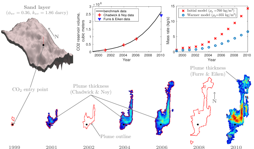
Figure 1. The Sleipner benchmark (sand layer, entry rates, fluid and rock properties) from [5], and CO₂ plume data taken from Chadwick & Noy [8] and Furre & Eiken [7]. While seismic imaging can estimate the volume of CO₂ in Layer 9, the rates depends on the inferred reservoir density; mass rates shown here are computed assuming densities of 760 and 355 kg/m³.

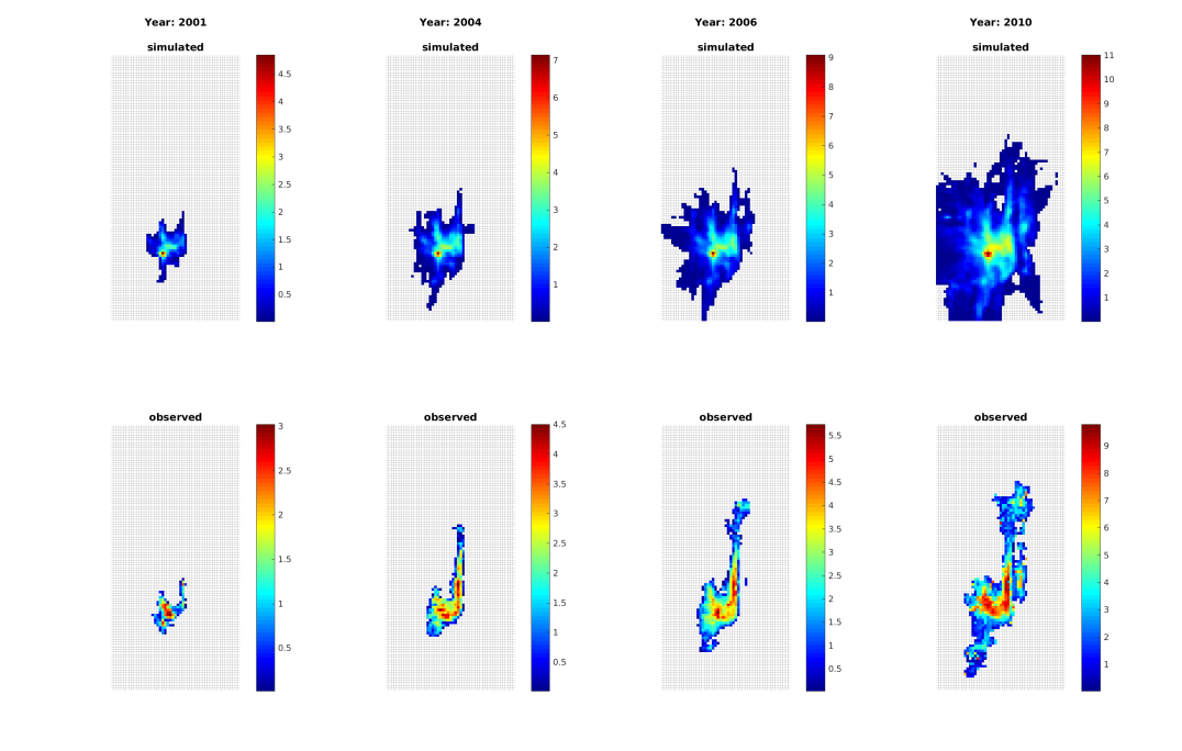
Figure 2. Comparing the original model with the plume data on the simulation grid used.

Figure 3. Comparing the matched model with the plume data on the simulation grid used.

3. The Sleipner Layer 9 (L9) benchmark model

We use the Sleipner L9 model based on the benchmark [5] with the exact definitions as in our previous work [6]. Similarly, we use four sets of observed plume heights $h_{\text{obs}}$ taken from results published by Chadwick and Noy [8] and Furre and Eiken [7]. From these heights, we determined the corresponding plume volumes at four observation times. An over view of the data is shown in Figure  1. To investigate how the response of the model change with different physical situations we use the original model and a member of the family of match models investigated in [6].

To find a unique matched model, we fixed the density of the model to $478\mathrm{kg}/\mathrm{m^{3}}$ and the porosity to $0.37$. The Figure 3 how the resulting model match the estimated plume heights form [8, 7]

The most prominent change in the model is that the product of density difference and permeability is changed significantly to achieve a stronger gravity segregation effect. The resulting matched model have a permeability of $13\,\mathrm{Darcy}$ and the volume rate is multiplied with a $0.92$.

4. Example:

4.1. Matching plume on Sleipner

In this paper we will investigate how the physical conditions in the aquifer influence the sensitivites of the model. We use the original assumption of the Layer 9 benchmark [5], as described in section 3 We now proceed to match our model to the data. We minimize the difference between using the same methods as in [19] given a set of parameters $\theta$ in the same way as with the linear least-square theory (22). The misfit objective (27) with observed plume heights $h_{\text{obs}}$ for the years 2001, 2004, 2006, and 2010 are used (the first three years of data are taken from [8], and the last year is from [7]). To find a unique matched model, we fixed the density of the model to $475\mathrm{kg}/\mathrm{m^{3}}$ and the porosity to $0.37$. The most prominent change in the model is that the product of density difference and permeability is changed significantly to achieve a stronger gravity segregation effect. The resulting matched model have a permeability of $11\,\mathrm{Darcy}$ and the volume rate is multiplied with a $0.91$. The match before and after the match is shown in Figure 2 and Figure 3.

4.2. Sensitivity to parameter changes

The sensitivities related to porosity, density, permeability, and rate must be handled with particular care since these variables are of different character even if we have chosen to define all of them as dimensionless multiplication factors of the original values. The starting point for this discussion is to consider the top surface as constant so that the changes in CO₂ thickness can be written as

(32) $$\mathrm{d}h=A_{m,t}\mathrm{d}\theta_{m},$$

the change in vertical gravity is similarly

(33) $$\mathrm{d}g_{z}=G_{m,t}\mathrm{d}\theta_{m}.$$

In the following we will only consider the changes taking place in the Layer 9, to illustrate the methods. For realistic use of gravity data however a simulation of all the layers is necessary since filtering out effects for a single layer is difficult due to the global nature of the gravity response. In addition we will consider the total mass know. This will not be the case for Layer 9, but will also require the simulation of all layers. The linear equations can then be added corresponding to equation (20).

(34) $$\mathrm{d}M=N^{T}\mathrm{d}\theta_{m}.$$

Here $\theta_{m}$ indicates the multiplicative variable of parameter $\theta$. We consider all years with equal weights and standard deviation for the height $\sigma_{h}=1$ m and for gravity we consider $\sigma=3\,\mu\mathrm{Gal}$. The values of the control parameters is non dimensional and relative to the original values. Table 4.2 confirm the analysis in section 2.3 that measurement of the plume shape give 2 approximate zero singular values. Gravity gives one, but adding the total mass as a last constraint gives a determined system. In particular for the original case, the plume shape helps in the two last singular values. This we attribute to the smaller sensitivity of the gravity measurements to plume shapes, which is important for determining part of the system. If we look at the singular vectors we see that the smallest singular value of gravity and total mass system is dominated by changes a combination of changes in porosity and permeability, However this in the case total mass is include this included the space of the lowest singular values of the plume shape.

	Original				Matched
P	193	153	0	0	249	103	0	0
G	556	32	27	0	427	139	30	0
P G	578	170	92	0	449	238	131	0
P M	1421	192	63	0	1931	239	67	0
G M	1445	470	29	13	1929	423	138	17
P G M	1453	490	137	50	1932	448	232

Table 1. Table over the singular values of all time steps for original and match model.Here P, G, and M stand for plume, gravity and total mass perspectively.

4.3. Sensitivity of topsurface data

We now investigate the sensitivity with regard to changes in the top-surface. This can be described by the relation

(35) $$\mathrm{d}h_{t}=A_{t}\mathrm{d}z,$$

where $\mathrm{d}h_{t}$ is the change in CO₂ thickness from the matched model corresponding to a change in the topsurface $\mathrm{d}z$ at a given time $t$-. In the previous paper we showed that $h+z$ was near constant, for situation near local equilibrium. We therefor also define modified matrices corresponding to mappings between parameters and linear combination of changes in CO₂ thickness and top surface

(36) $$\mathrm{d}h+\mathrm{d}z=A_{s,t}\mathrm{d}z\quad A_{s,t}=A_{t}+I$$

$A_{s,t}$, can be seen as calculating the sensitivity with respect to the water-CO₂ interface instead of the CO₂ height.

Original	Matched

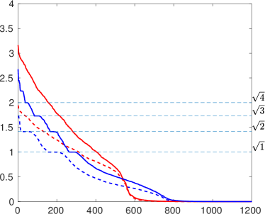
Figure 4. The singular values of the full sensitivity. Red color signifies for $h$, i.e. plume observation while the blue color is for $\mathrm{d}z$, interface observations. Full line is using all steps while the dashed line is using steps $1,5,9,12$.

Original	Matched

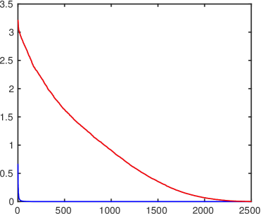
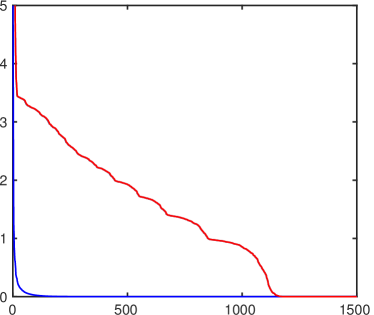
Figure 5. The singular values of the full sensitivity. Red color signifies for plume observation while blue color is gravity, $h$.

Figure 4 shows the singular for all time steps full line and only including time steps of year $1$, $5$, $9$,and $12$, dashed line. The red line is the sensitivites for plume height blue is for the CO₂-water. We notice the much stronger sensitivites of the match model for plume shape, while much less sensitivites for the CO₂-water interface. This is since the CO₂-water interface dynamics is only sensitive to the large scale features in the well segregated model, in analogy with that a lake surface do not depend on the bottom shape. On the other hand for the original model where gravity is much less important the sensitivity to the interface of the plume shape is almost equal. In this case the potential roughness of the top CO₂-water interface will not be smoothed by the plume dynamics and topsurface altrations my be recognized in the interface dynamics.

If compare the sensitivities of the plume shape with the sensitivity of the gravity measurement for the top surface, we see that there the gravity have a fast decay, Figure 5. There is hence very little part of the top surface changes which have significant impact on the gravity response. This may be expected since gravity only notice topsurface changes which contrite to significant global changes in shape. Even more it must lead to significant changes in integrated quantities, see equation 7

in 9

	Max min SVD	D-optimal	Mutual information
Original
Matched

Figure 6. Comperaing different optimal design criterieas including timestep $1$,$5$,$9$ and $10$. The optimal points shown in red is for step $\n$

in 1

	$U_{2}$	$U_{3}$	$U_{4}$
Plume
Gravity

Figure 7. Optimal design for the original model with standard with the original assumption of the errors for gravity and plume data. The red squares show the optimal design usind D-optimal criteria with $20$ possible observation. The upper row show the response singular value corresponding to plume and the lower row for the gravity. The columns represent the second, third and forth singular value.

in 10

	$U_{2}$	$U_{3}$	$U_{4}$
Plume
Gravity

Figure 8. The same as Figure 7, but for the matched model and assuming standard deviation of gravity is $10$ times less.

in 1 in optimum

	$U_{2}$	$U_{3}$	$U_{4}$
Plume
Gravity

Figure 9. The same as Figure 8 assuming observations of plume is in stripes. The standard deviations are the originally but the stripes are weighted with the number of cells.

in 1 in optimum

	$U_{2}$	$U_{3}$	$U_{4}$
Plume
Gravity

Figure 10. The same as Figure 8 assuming observations of plume is in stripes. The standard deviations are the originally but the stripes are weighted with the number of cells.

Figure 11. The figure show the time-dependence of the accumulated svd of plume in blue, gravity in red and total mass in light brown with respect to the global parameters. The left is the using the direct observations. While the right show the same for using changes between time steps.

5. Optimal design of experiment

We now continue with the question of which of the parameters which make most contributions to the observations. This depend on the cost and accuracy of different measurement technologies. For example in the case of seismic one have the choises between 2D, 3D with repeated survies or stationary sensors. 3D is seen as the most cost efficient for deep aquifers with in the context of oil exploration at an approximate cost of 10000  $/km². The cost of 2D seismic is 5000  $/km². However the cost to benefit evaluation in the context of oil extrapolation is not directly applicable to CO₂ monitoring. The stationary case will in most cases have better repeatability which may contribute to significant increase of accuracy in estimation when a reservoir model is to be estimated. Gravity is considered to be a cheaper for a given area. Often it is referred that the cost is reduced by a factor of 10, but to our knowledge a estimates taking into account the different information of the two services has not been published. The advantage is that it directly measures model changes, but it have smaller sensitivity to small spatial changes in the plume which may be important for detecting leakage pathways early. In the below we will only consider question of who to choose the observation from a traditional optimal design of experiment perspective and not take cost and accuracy of the different methods quantitatively into account by scaling the importance of gravity with regard to plume shape. For a proper evaluation in the case of plume shape it would have been necessary to include the seismic inversion, since this will more directly be related the physical devices which decide the cost of the measurements.

5.1. Plume shape data

We first look directly on the plume shape data and compare the different methods of optimal design using the timesteps $1$,$5$,$9$ and $12$. We make the rather unrealistic assumption of been able to choose observations independently in different grid cells. As expected the most important time steps is the last ones. The contributions from time step $9$ is shown in Figure 6. We see that all optimal design criteria highlights the outline of the plume in the matched case. The effect is less pronounced for the original case. Another important feature is that it divides the points used between the different compartments. As discussed above the use of point data do not honor the way data is collected and certainly not how the preprocessing step of seismic inversion is done. A more fair use although simplified is to say that the each observation is either a slice in the x-direction or/and y-direction. We will consider this when including gravity data.

In all of these cases, we see that the different optimal design criteria give approximately the same value. In terms of computational cost the ones based on continuous optimization are most efficient, while the mutual information based method give slightly more robust points form a qualitative viewpoint. The method based on disciplined convex programing seemed more stable for large systems. This may be due to the slightly simpler D-optimal criteria. The interior point based algorithm is much simpler to extend to a cost based optimization However convexity and a guaranty to find the global optimum can not be known a priory. For the rest of the paper we will stick the the computational attractive D-optimal criteria.

5.2. Optimal design for gravity and plume shape data

We know look at the effect of combining plume shape and gravity data together. To form a complete system for the global parameters and to be more realistic for a full system, we restrict us to the case where the total mass is known accurately. We consider two different scenarios. One where we us the unchanged sensitivities and one where we multiply the gravity sensitivity with a factor $10$. Figure 7 and 8 show the results for the original model with factor $1$ and the matched model factor $10$ respectively, using time step 9. First we notice the the placement of the gravity observations is more prone centered than for the plume data. This we attribute to the global smooth character of the gravity response. Secondly we observe that in the case where it is favorable to have many gravity observation, Figure 8, the gravity observations is placed to be sensitive to the multipole expansion of the gravity response. We also see that even with this low weight of the plume data it is still favorable to keep some of this observation. In particular the observations on the other side of the main spill point is favored. The colors of the figure give the strength for different singular value in each columns and the two rows response singular vector for the plume upper row and gravity lower row. We see that the two first singular values in the high gravity sensitivity case, Figure  8, are dominated monopole and the dipole contribution respectively.

The assumption of being able to choose the estimates of the plume shape freely in space is not realistic both with respect to who seismic data is collected offshore and also with the preprocessing step needed estimating the plume shape from raw seismic wavefields. To make the optimal design somewhat more realistic without introducing seismic inversion we restrict observations of the plume to be either in horizontal strips or in vertical strips. We weight the observations with the number of points in a strips. This would correspond to letting the cost of one strip be proportional to the length. Figure  9 show the result for the matched case with equal original weight. This is still a case which slightly favoring gravitational measurements, but we see that the two slices of the plume are chosen in the region where the plume is thickest.

5.3. Effect of diffential measurements

For many measurements more accuracy can be obtained for differences than for a given value. This is particular the case for technologies with high repeatability and small drift. In the case of monitoring CO₂ this will in particular be the case for certain types of gravity measurements. Passive monitoring systems for seismic waves where position of the hydrophones is the same all the time will also potentially benefit from processing which can utilize the this feature. Given our linearized model the advantages of large repeatability can be evaluated using

(37) $$\mathrm{d}(y_{i+1}-y_{i})=(A_{i+1}-A_{i})\mathrm{d}\theta$$

If the errors associated with measurements of $y_{i+1}-y_{i})$ is significantly less than for the original quantities large gains can be achieved, if the measurements are linear independent with regard to the parameters. That is $A_{i+1}$ is significantly different from $A_{i}$. Figure 11 show the evolusion of the svd of the accumulated system using observation of absolute changes left and differential changes right. Given that the measurements system have more than $4$ times lower standard deviation for differential measurement, that will give more information.

5.4. Effect of resolution

The framework may become computational challenging when the resolution is increased. Figure  10 show the same results as in Figure 9 but with a coarser resolution. We see that the optimal design is qualitatively the same. We have seen the same feature for most of the cases we have run. Some discrepancies is found when resolution changes the behavoir of the plume. Most prominently when the upward flowing feature is underestimated due to low resolution.

6. Discussion

When considering an optimal monitoring strategy one has to consider the cost of a measurement, how much it contributes to the knowledge of the system and how valuable the information is. The cost is most often known, but quantifying how well one can estimate the system given a set of measurements is difficult. This requires a model of the system and the measurement methods. For accurate estimation one also need a good estimation of the errors and covariance of the error (even neglecting the difficulties of nonlinearities.) This may include pure stochastic errors of the measurement process, but more often it is associated with uncertainties in parameters of the measurement process (i.e. inverse modeling errors) which often depend on unknown geology. Some of this parameters have very large variations like permeability, and some have less variation like density of stone. However how important the variation is for the system is highly dependent on the system. A key point is the covariance of the errors of a measurement and the linearly independence of them. Roughly speeking correlation is good for linearly independent measurements but bad for linearly dependent measurements. To evaluate the value of the information one in addition have to connect the information with a value of a decision process. The latter is a difficult question in itself for CO₂ storage, which only have indirect value and the responsibility of may be shared between different stakeholders.

Instead of starting from the measurement process we have in this paper investigated the question from the simplest simulation model which has been demonstrated to simulate CO₂ plume dynamics accurately in certain situation, most prominently the Sleipner L9 case. The motivation has been to look at the sensitivity of this simple model and connect this to observation, although in an indirect way in the case of plume shape. With this simplification we have been able to calculate full linear models from the parameters of the nonlinear model to the observations. This has made it possible to investigate both how knowledge of the plume dynamics and gravity response relate to the model parameters. In particular we could exploit the power of the SVD compositions. In addition, it made it possible to investigate the monitoring problem efficiently in the setting of optimal design. We consider this to be a starting point for optimization of the monitoring strategy with respect to accuracy constraints. Furthermore our work should be extended for optimizing the monitoring framework so that it is robust with respect to the assumed uncertainties. As we have demonstrated in the Sleipner L9 case the naive answer to the optimal design question is significantly different between the original assumed model and what we today believe is the reality. A monitoring policy should therefor be robust and with respect to this initial large uncertainty.

In addition to the theoretical difficulties of the problem in itself we have the question: Is the problem computational feasible? We have here not included the seismic inversion process which is a large computation challenge in it self, we believe could benefit form a direct coupling with the flow modeling in particular if the inversion is targeted to changes. We have used a VE based simulation model with and restricted the uncertainties of the model to rather few parameters. Extending this model will contribute to increased computation cost, in particular if full 3D model is required. However we believe that extensions to layered models will be sufficient form many cases. Also the assumption of uniform uncertainty of permeability will in many cases be to simplistic. However both of this problems contribute to increasing the computation of the above frame work, they do grow approximately linearly due to the use of adjoint bases sensitivities. When combined with full linearization of the system which also grow linearly with the number of observation it may be quite restrictive. The linearization will most often lead to dens systems. This may be challenging for a strait forward full evaluation of the SVD decomposition. However the observations is independent of the grid gridding and may be restricted. SVD analysis can also give valuable information about particular subspaces. Coarse grids in combination with VE based models is also likely to give good result due to the strong parabolic term in this equation. In addition to the challenge of including nonlinear and robust optimization in a statistical sense, the critical part is if the problem of optimal design can be done if the model complexity is larger. We believe this is less computation demanding than the full SVD calculations. In addition one would in most cases not seek full free optimization like in Figure 8 and 7 but rather restrict for example the possible configurations to strips and a few points like in 9. This reduce the computational cost significantly and make the framework valuable to evaluate cost versus benefit at least for restricted combination of measurements.

7. Conclusion

In the setting of CO₂ monitoring we have used flow simulations with adjoint based sensitives and shown how efficient the different monitored variables are to estimate a simulation model. In particular we have by using an efficient VE-based simulation model shown that different physical scenarios thought to be plausible for the Sleipner Layer 9 have different qualitatively with respect to the sensitivity to monitored quantities. We showed that the main parameters of our model could be estimated if gravity response and total mass is known. Plume shape and total mass is, however not sufficient. But plume-shape gave significant additional benefit even not sufficient in it self.

We also used the framework to evaluate the estimated quantities in a setting of optimal design. Although not giving quantitatively estimate of efficient monitoring strategies this gave insight into which part of the estimated quantities are most important for estimating the flow model. With the simplified model for accuracy the optimal design gave high weights to the plume outline while the important part of the gravity response was the main multipoles. As gravity response is global and effectively isolated to the change in CO₂ volume times the density difference to water, it seems like an ideal candidate to robustly monitor the main part of the CO₂ dynamics. Little assumption of the overburden is also needed, although separating the gravity changes of the CO₂ to other sources may be difficult without a proper simulation model which can give strong restrictions on how gravity should change both in time and space. Our results indicate that gravity measurements should be a valuable part of a monitoring program details of the plume shape give important complementary information and a combination is likely to be the most efficient. In a scenario where cost is introduced our results indicate that limited accurate observations will give the most cost efficient and robust monitoring strategy. But more in-dept study using realistic cost to accuracy, including models for seismic inversion is needed to establish this further. When a reliable dynamic model can be formulated the result indicate that observation with high accuracy on differential measurements will be favorable.

In this paper we discussed the use of optimal design in the simplified setting of Sleipner Layer 9. In more difficult cases where strong restrictions of the injectivity, possibility of activation of near by faults measurements related to pressure would probably be favorable. The possible global measurements are in such case uplift or possible micro-seismic activity. Both will most likely favor stationary passive systems. Uplift which my be readily included in our framework will be most sensitive to differential measurements with high accuracy, since this can be attributed directly to pressure changes in a similarly to gravity, this is contrary to seismic and electromagnetic measurements where where only measure changes in the media indirectly. Mico seismics also look at a source to the signal directly, but here the source is more indirectly assosiated with the CO₂ injection.

We believe the computational tools and methods used here in the setting of CO₂ storage will contribute to finding cost efficient monitoring programs for CO₂ storage.

Acknowledgements

This work was funded in part by the Research Council of Norway through grant no. 243729 (Simulation and optimization of large-scale, aquifer-wide CO₂ injection in the North Sea).

Statoil and the Sleipner License are acknowledged for provision of the Sleipner 2010 Reference dataset. Any conclusions in this paper concerning the Sleipner field are the authors’ own opinions and do not necessarily represent the views of Statoil.

References

- [1] E. K. Halland, W. T. Johansen, F. Riis (Eds.), CO2 Storage Atlas: Norwegian North Sea, Norwegian Petroleum Directorate, P. O. Box 600, NO–4003 Stavanger, Norway, 2011.
- [2] M. Ravasi, I. Vasconcelos, A. Kritski, A. Curtis, C. A. d. C. Filho, G. A. Meles, Target-oriented marchenko imaging of a north sea field, Geophysical Journal International 205 (1) (2016) 99.
- [3] A. Romdhane, E. Querendez, CO2 characterization at the Sleipner field with full waveform inversion: Application to synthetic and real data, Energy Procedia 63 (2014) 4358–4365.
- [4] B. Dupuy, S. Garambois, A. Asnaashari, H. M. Balhareth, M. Landrø, A. Stovas, J. Virieux, Estimation of rock physics properties from seismic attributes — part 2: Applications, Geophysics 81 (4) (2016) M55–M69.
- [5] V. Singh, A. Cavanagh, H. Hansen, B. Nazarian, M. Iding, P. Ringrose, Reservoir modeling of CO2 plume behavior calibrated against monitoring data from Sleipner, Norway, in: SPE Annual Technical Conference and Exhibition, Florence, Italy, 2010.
- [6] H. M. Nilsen, S. Krogstada, O. Andersena, R. Allena, K.-A. Lie, Using sensitivities and vertical-equilibrium models for parameter estimation of co2 injection models with application to sleipner data, Energy Procedia.
- [7] A. K. Furre, O. Eiken, Dual sensor streamer technology used in Sleipner CO2 injection monitoring, Geophysical Prospecting 62 (5) (2014) 1075–1088.
- [8] R. Chadwick, D. J. Noy, History-matching flow simulations and time-lapse seismic data from the Sleipner CO2 plume, in: Proceedings of the 7th Petroleum Geology Conference, Geological Society, London, 2010, pp. 1171–1182.
- [9] H. M. Nilsen, K.-A. Lie, O. Andersen, Robust simulation of sharp-interface models for fast estimation of CO2 trapping capacity, Computational Geosciences 20 (1) (2016) 93–113.
- [10] J. D. Jansen, Adjoint-based optimization of multi-phase flow through porous media – a review, Computers & Fluids 46 (1, SI) (2011) 40–51.
- [11] C. Paige, The general linear model and the generalized singular value decomposition, Linear Algebra and its Applications 70 (1985) 269 – 284.
- [12] M. Grant, S. Boyd, CVX: Matlab software for disciplined convex programming, version 2.1, http://cvxr.com/cvx (Mar. 2014).
- [13] A. Wächter, L. T. Biegler, On the implementation of an interior-point filter line-search algorithm for large-scale nonlinear programming, Mathematical Programming 106 (1) (2006) 25–57.
- [14] M. B. Giles, Collected Matrix Derivative Results for Forward and Reverse Mode Algorithmic Differentiation, Springer Berlin Heidelberg, Berlin, Heidelberg, 2008, pp. 35–44.
- [15] M. Giles, An extended collection of matrix derivative results for forward and reverse mode algorithmic differentiation, 2008, pp. 1–22, https://people.maths.ox.ac.uk/gilesm/files/NA-08-01.pdf.
- [16] S. F. Walter, L. Lehmann, Algorithmic differentiation of linear algebra functions with application in optimum experimental design (extended version), CoRR (2010) abs/1001.1654.
- [17] A. Krause, A. Singh, C. Guestrin, Near-optimal sensor placements in gaussian processes: Theory, efficient algorithms and empirical studies, J. Mach. Learn. Res. 9 (2008) 235–284.
- [18] A. Krause, Sfo: A toolbox for submodular function optimization, J. Mach. Learn. Res. 11 (2010) 1141–1144.
- [19] R. Allen, H. Nilsen, O. Andersen, K.-A. Lie, On obtaining optimal well rates and placement for co2 storage, in: ECMOR XV – 15th European Conference on the Mathematics of Oil Recovery, EAGE, 2016.