QCD phase diagram for nonzero isospin-asymmetry
Abstract
The QCD phase diagram is studied in the presence of an isospin asymmetry using continuum extrapolated staggered quarks with physical masses. In particular, we investigate the phase boundary between the normal and the pion condensation phases and the chiral/deconfinement transition. The simulations are performed with a small explicit breaking parameter in order to avoid the accumulation of zero modes and thereby stabilize the algorithm. The limit of vanishing explicit breaking is obtained by means of an extrapolation, which is facilitated by a novel improvement program employing the singular value representation of the Dirac operator. Our findings indicate that no pion condensation takes place above and also suggest that the deconfinement crossover continuously connects to the BEC-BCS crossover at high isospin asymmetries. The results may be directly compared to effective theories and model approaches to QCD.
I Introduction
The thermodynamics of strongly interacting matter, as described by quantum chromodynamics (QCD), plays a characteristic role for the phenomenology of heavy-ion collisions, the structure of compact stars and the evolution of the early Universe. The relevant parameters that impact QCD physics in these settings include the temperature and the net densities of the individual quark flavors . In the light quark sector (), the characteristic combinations are the baryon density and the isospin density . While the former measures the overall excess of strongly interacting matter over antimatter, the isospin density describes the asymmetry between the up and down quarks or, equivalently, between protons and neutrons in the system.
The above-mentioned physical settings are all thought to exhibit a strong isospin asymmetry. The initial state of typical heavy-ion collisions has around twice as many neutrons as protons, which has implications, for example, for the imbalance between the generated charged pions Li et al. (1998). Cold neutron stars are characterized by even lower proton fractions Steiner et al. (2005). A high isospin asymmetry is carried by charged pion degrees of freedom that might be relevant for compact stars or for nuclear matter in general Migdal et al. (1990). Although the early Universe is typically assumed to undergo an evolution with almost vanishing densities, a large lepton asymmetry might propagate into the baryon sector and shift equilibrium conditions around the time of the QCD transition Schwarz and Stuke (2009).
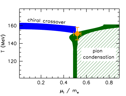
In the grand canonical approach to QCD, the densities are traded for the corresponding chemical potentials and the isospin chemical potential is defined as . The phase diagram in the temperature – isospin chemical potential plane is known to exhibit at least four different phases that can be relevant for the physical systems mentioned above. We discuss these phases qualitatively in Fig. 1. In the vacuum (for low values of and of ) QCD is confining and the effective degrees of freedom are hadrons. On the one hand, if the temperature is raised at low isospin chemical potential, deconfinement sets in and the quark-gluon plasma phase is realized. Lattice QCD simulations have demonstrated that the transition to deconfinement is an analytic crossover Aoki et al. (2006a); *Bhattacharya:2014ara and occurs near the chiral pseudocritical temperature of Borsányi et al. (2010); *Bazavov:2011nk. On the other hand, if is increased at low temperature, another phase transition line is encountered, which can be best understood using an effective description of QCD based on pionic degrees of freedom. Charged pions are the lightest hadrons that couple to the isospin chemical potential, and their effective dynamics is described by chiral perturbation theory (PT) Son and Stephanov (2001).
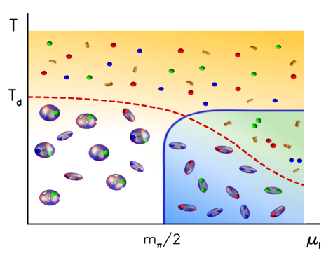
At , if the isospin chemical potential exceeds the critical value , sufficient energy is pumped into the system so that charged pions can be created. Due to the bosonic nature of pions, a Bose-Einstein condensate (BEC) is formed at this point. PT also predicts that the transition between the vacuum and the BEC state is of second order with the universality class Son and Stephanov (2001). As is usually the case, the temperature tends to destroy the condensate so that this phase transition line is expected to bend towards higher values of as grows. While PT predicts a monotonous rise of , our preliminary lattice simulations reveal a flattening of this curve around the zero-density deconfinement crossover Brandt and Endrődi (2016); Brandt et al. (2017). This suggests that deconfinement is in some sense stronger than the condensation mechanism, and in the quark-gluon plasma phase no pions can be created by increasing .
Yet another transition is expected to occur at even higher isospin chemical potential. Perturbation theory predicts that the attractive gluon interaction forms Cooper-pairs (BCS superconductivity) of and quarks in the pseudoscalar channel. Since the resulting pair has the same quantum numbers as the pion condensate, the deconfinement-type transition between the BEC and BCS states is expected to be an analytic crossover Son and Stephanov (2001).
The particular structure of the transition lines separating these four phases (hadronic, quark-gluon plasma, BEC and BCS) in the phase diagram is not yet known. The results we present below favor the scenario depicted in Fig. 1, where the deconfinement transition continuously connects to the BEC-BCS crossover at high isospin chemical potentials. We note that for asymptotically large values of , perturbative arguments suggest Son and Stephanov (2001); Cohen and Sen (2015) a decoupling of the gluonic sector and the emergence of a first-order deconfinement phase transition. This region is not included in Fig. 1.
The QCD phase diagram at nonzero temperature and isospin chemical potential has been studied using a multitude of approaches. Besides the already mentioned chiral perturbation theory as effective description Son and Stephanov (2001); Splittorff et al. (2001); *Loewe:2002tw; *Fraga:2008be; *Janssen:2015lda; *Carignano:2016lxe, hard thermal loop perturbation theory Andersen et al. (2016) and different low-energy models of QCD have been employed. The latter include the Nambu-Jona-Lasinio (NJL) model in four Toublan and Kogut (2003); *Frank:2003ve; *Barducci:2004tt; *He:2005sp; *Zhang:2006gu; *Sun:2007fc; *Xia:2013caa; *Zhang:2015baa; *Brauner:2016lkh; *Khunjua:2017mkc and in two dimensions Gubina et al. (2012), the linear sigma or quark meson model He et al. (2005); *Ueda:2013sia; *Stiele:2013pma, scalar field theory Andersen (2007), random matrix models Klein et al. (2003), the thermodynamic bag model Klahn et al. (2017), the hadron resonance gas model Toublan and Kogut (2005) and by means of the functional renormalization group or Dyson-Schwinger equations Zhang and Liu (2007b); *Svanes:2010we; *Kamikado:2012bt; *Wang:2017vis. The impact of the isospin chemical potential was also investigated in the limit of large number of colors Kashiwa and Ohnishi (2017) and employing the holographic principle Aharony et al. (2008); *Basu:2008bh; *Albrecht:2010eg. For large , the phase diagram was argued to be related to the analogous phase diagram with baryon chemical potential via the orbifold equivalence Hanada and Yamamoto (2012). In particular, this equivalence is expected to hold outside the pion condensation phase only, so that the precise knowledge of the location of the BEC transition line is relevant from this point of view as well.
A significant advantage of the system is that – unlike for nonzero baryon chemical potential – there is no sign problem and lattice QCD simulations can be employed to investigate the phase diagram directly. Following the pioneering work of Refs. Kogut and Sinclair (2002a, b), the phase diagram was studied both in the grand canonical Kogut and Sinclair (2004); Cea et al. (2012); Endrődi (2014) and in the canonical ensemble de Forcrand et al. (2007); Detmold et al. (2012). The low isospin density region was also discussed by means of a Taylor expansion in Allton et al. (2005); Borsányi et al. (2012a), while the strong coupling regime was investigated using the strong coupling expansion Nishida (2004); *Langelage:2014vpa. Finally, we mention that QCD with has deep relations to two-color QCD with baryon chemical potentials. The latter theory has also been the subject of intensive research, both on the lattice Kogut et al. (2001); *Hands:2006ve; *Bornyakov:2017txe as well as in model and functional approaches Andersen and Brauner (2010); *Strodthoff:2011tz; *vonSmekal:2012vx.
We mention that, besides the broad range of applications for this system, an additional motivation to study the theory is its similarity with nonvanishing baryon chemical potential, , both on the conceptual and on the technical level. At , both systems exhibit the so-called silver blaze phenomenon Cohen (2003) and undergo a phase transition from the vacuum to a phase where colorless composite particles are created. This transition is accompanied by the accumulation of near-zero eigenvalues of the fermion matrix in both cases, leading to an ill-conditioned inversion problem and a breakdown of naive simulation algorithms. This necessitates the use of an infrared regulator that we denote by below. Understanding these concepts and facing these technical challenges in the (sign-problem-free) theory may give us insight on how to assess the system in the future.
In this paper we follow the grand canonical approach and simulate QCD with flavors of dynamical staggered quarks at various values of and . Besides the inclusion of the strange quark, we improve over currently existing studies in the literature by using physical quark masses and employing an improved lattice action in the simulations. The latter enables a faster scaling towards the continuum limit. Furthermore, we present a novel method to perform the extrapolation of the infrared regulator to zero – the main technical achievement in this project. This method involves the singular values of the massive Dirac operator, which we discuss for the first time on the lattice in this context. Preliminary results of our simulations were presented in Refs. Brandt and Endrődi (2016); Brandt et al. (2017) and applied in Ref. Bali et al. (2016).
II Setup and observables
II.1 Symmetries
First of all, it is instructive to discuss the pattern of the symmetry breaking that leads to Bose-Einstein condensation at high isospin chemical potentials. In Euclidean spacetime, our choice for the continuum action for the light quarks includes
| (1) |
Here is the gluon field and denote the Pauli matrices. Besides the isospin chemical potential and the quark mass , we also included an explicit symmetry breaking term in that couples to the charged pion field ,
| (2) |
The role of the parameter – referred to as a pionic source in the following – will be elucidated below.
At (but nonzero , the action is symmetric under the chiral group . The symmetry, corresponding to baryon number conservation, is not affected by the chemical potential nor by the pionic source and is not discussed in the following. The symmetry group is broken down to by the chemical potential. The subscript indicates that the generator of the remaining symmetry is . Pion condensation is signaled by the spontaneous breaking of this symmetry, by any of the expectation values , .
The spontaneous breaking of the continuous symmetry implies the presence of a Goldstone mode. The introduction of the pionic source in (1) corresponds to an additional explicit breaking that selects the direction for the ground state and makes the would-be massless mode a pseudo-Goldstone boson. In fact, in a finite volume, such a trigger is necessary for the spontaneous breaking to occur. The physical limit is obtained subsequently by means of an extrapolation. Notice that for the symmetry, its spontaneous (by ) and explicit (by ) breaking is completely analogous to the one of the standard chiral symmetry at , together with its spontaneous (by ) and explicit (by ) breakings. One very important difference is that while in nature , the parameter is unphysical and the limit needs to be taken.
For vanishing isospin chemical potential, the pionic source can be rotated into the mass parameter. In particular, we can perform the chiral rotation
| (3) |
This rotation brings the action into a flavor-diagonal form
| (4) |
Thus, at the mass and the pionic source parameter are indistinguishable and only their squared sum plays a physical role. This will have important consequences for the ultraviolet structure of the theory, see Sec. II.3 below. Notice that for the pionic source has the same interpretation as the twisted mass parameter used in the context of Wilson fermions Frezzotti et al. (2001).
II.2 Lattice setup
To investigate pion condensation and the associated spontaneous symmetry breaking, we study 2+1-flavor QCD with and nonperturbatively on the lattice. We work on lattices with spacing and sites indexed by the coordinates . The temperature and the spatial volume read and , respectively. To discretize the Dirac operator we use the staggered formulation; here the equivalent of is the local spin-flavor structure . At , this operator couples to the Goldstone boson in the chiral limit.
The partition function of this system is given in terms of the path integral over the gluon links ,
| (5) |
where we employed the rooting procedure (for a discussion on the theoretical issues related to rooting, see Ref. Dürr (2006)). In Eq. (5), denotes the inverse gauge coupling, is the tree-level Symanzik improved gluon action, is the light quark matrix in the basis of the up and down quarks and is the strange quark matrix,
| (6) |
Here, the argument of indicates the chemical potential , introduced on the lattice by multiplying the forward (backward) timelike links by (). The pionic source parameter induces an explicit symmetry breaking and serves to trigger pion condensation as we discussed above in Sec. II.1.
The integrand of needs to be positive to allow the importance sampling of the gluon configurations. The strange quark determinant is real and positive due to the standard -hermiticity relation . To show the positivity for the light sector, we need to discuss the symmetry properties of the staggered Dirac operator at . The staggered equivalent of chiral symmetry implies that
| (7) |
holds. In addition, the Dirac operator satisfies
| (8) |
so that the light fermion matrix is -hermitian
| (9) |
Thus, taking the determinant of both sides shows that is real.
One can also show that the determinant is positive by considering
| (10) |
where and we used Eq. (8). Indeed, since has unit determinant, we have
| (11) |
Thus, both determinants in the measure of the path integral (5) are positive.
The fourth root of the determinants in (5) is approximated via rational functions. The simulation setup with was first introduced for the theory in the pioneering work of Ref. Kogut and Sinclair (2002a) for the quenched case and in Ref. Kogut and Sinclair (2002b) for dynamical QCD. The same technique was also used in Ref. Endrődi (2014). Here we extend this setup by including the strange quark as well. In addition, we improve the lattice action by using the tree-level Symanzik gauge action and by employing two steps of stout smearing in the Dirac operator. The quark masses are tuned to their physical values along the line of constant physics (LCP) , as determined in Ref. Borsányi et al. (2010), with the pion mass . Our simulation algorithm is based on Ref. Aoki et al. (2006b). In addition we implement a Hasenbusch-type improvement scheme that is typically used in the context of mass preconditioning Urbach et al. (2006). In our setup this amounts to the replacement with , which allows to use a larger step size (and a lower precision) in the simulation algorithm for the second (more expensive) factor.
II.3 Observables and renormalization
Our primary observables are the pion condensate and the quark condensate. Both are obtained from the partition function via differentiation,
| (12) |
Inserting the partition function (5) and rewriting the light quark determinant using Eq. (11), we obtain for the condensate operators,
| (13) |
The relation (13) allows for direct measurements using noisy estimators.
The observables of Eq. (12) are subject to additive renormalization. This is necessary, since contains ultraviolet divergences in the inverse lattice spacing. The structure of these divergences can be determined based on dimensional arguments (see Ref. Leutwyler and Smilga (1992) for a discussion at ),
| (14) |
where we suppressed further divergences that contain . Note that the divergences are independent of , since the chemical potential couples to a conserved charge Hasenfratz and Karsch (1983). Thus, it suffices to consider the case of . Above in Eq. (4) we have seen that for vanishing isospin chemical potential, the mass and the pionic source may be rotated into each other, so that the two parameters can only appear in Eq. (14) in the form . The quark condensate and the pion condensate inherit the quadratic and the logarithmic divergences from . However, for these vanish at – the point of interest for the physical theory. Since the light quark mass is nonzero, the additive divergences remain in and need to be subtracted even in the limit . The standard choice is to consider the difference to measured in the vacuum, i.e. at .
Finally we need to address the multiplicative renormalization of our observables. The quark condensate and the pion condensate have nontrivial renormalization constants, and . The equivalence of and at and the -independence of the renormalization constants, however, imply that , so that a multiplication of the condensates by cancels the multiplicative divergence.111Note that multiplying by would also result in a renormalization group invariant combination. However, this construction vanishes in the limit and is therefore not useful. Altogether, the renormalized observables read
| (15) |
where we also included a normalization factor involving the pion mass and the chiral limit of the pion decay constant and added unity to the quark condensate for convenience. In this normalization (which follows Ref. Bali et al. (2012)), at due to the Gell-Mann-Oakes-Renner relation. In addition, zero-temperature leading-order PT Son and Stephanov (2001) predicts a gradual rotation of the condensates so that holds irrespective of , which can also be observed to some extent in the full theory.
In addition to the fermionic observables we also consider the Polyakov loop,
| (16) |
as a measure for deconfinement. The multiplicative renormalization of amounts to
| (17) |
with an arbitrary choice for and . Different choices correspond to different renormalization schemes; we choose , where the bare Polyakov loops are already significantly nonzero, and set . This renormalization prescription for was developed at Borsányi et al. (2012b) and also put into practice at nonzero background magnetic fields Bruckmann et al. (2013).
III Improvements for the extrapolation
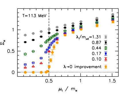
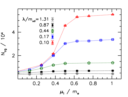
The pionic source parameter is introduced in order to trigger pion condensation and to stabilize the simulation algorithm. However, in order to obtain physical results needs to be extrapolated to zero. Most of the observables exhibit a pronounced dependence on , making this extrapolation cumbersome. As a typical example, in the top panel of Fig. 2 we show the pion condensate of Eq. (15) as measured using various values of on our ensembles at . Especially below and around the critical chemical potential , a direct fitting of the data appears to be hopeless. This necessitates various improvements, both in the valence sector (the definition of the operators) and in the sea sector (reweighting of the configurations), to eliminate the -dependence in the observables. The result of the improvement, which we will describe below, is also included in the top panel of Fig. 2 – clearly revealing the transition between the vacuum and the BEC phase, which was hidden for the direct data at high .
The simulations at low values of suffer from a numerical problem. Since the pionic source acts as an infrared regulator, it has a substantial impact on the condition number of the fermion matrix . In particular, the average iteration count for the convergence of the conjugate gradient algorithm used for inverting grows significantly as decreases. This is especially the case in the pion condensed phase (see the bottom panel of Fig. 2), where the inversion at our smallest is an order of magnitude slower than at the largest pionic source.222We also mention that simulating with is not feasible even for our smallest isospin chemical potentials due to the occasional appearance of configurations with fermion matrices of very high condition numbers, for which the numerical inversion breaks down. Moreover, in order to maintain a reasonable acceptance in the Metropolis step, the simulations at low need to be performed with a reduced step size along the Monte-Carlo trajectory due to increasing fluctuations in the fermion force. This leads to a slowing down by a further factor of for the lowest pionic source.
Thus, improving our observables so that they lie closer to their limit is necessary – both for controlling the extrapolation and for sparing simulation time. It turns out that the improvement for the pion condensate is drastically different from the improvement of the other observables due to the fact that plays the role of the order parameter for Bose-Einstein condensation and thus has a highly nontrivial finite volume scaling. There is, nevertheless, a common element in the improvement program, which is the singular value representation of the massive Dirac operator.
III.1 Singular values
To get acquainted with the notion of singular values, let us begin with the eigenvalue equation of the massive Dirac operator. For the up quark, the eigensystem reads
| (18) |
where the eigenvalues are complex numbers. Using chiral symmetry (7) and the hermiticity relation (8) we obtain the eigensystem for the down quark,
| (19) |
Note that is not a normal operator thus and its left and right eigenvectors do not coincide. Nevertheless, Eqs. (18) and (19) reveal that for each eigenvalue in the up quark sector there is a complex conjugate pair in the down quark sector, which is why the determinant of the total light quark matrix is real and positive as we have seen in Sec. II.2.
We can create a hermitian operator by taking the modulus squared of the Dirac operator Kanazawa et al. (2011). The square roots of the eigenvalues of this operator are referred to as the singular values333The name refers to the role of these in the singular value decomposition of non-hermitian matrices. of the Dirac operator. The eigenvalue equation reads
| (20) |
Note that due to the non-normality of , there is no relation between the singular values and the eigenvalues . We note that the singular values of and of coincide due to the hermiticity relation (8).
III.2 Banks-Casher type relation for the pion condensate
An important characteristic of chiral symmetry breaking at is reflected by the Banks-Casher relation Banks and Casher (1980), which states that the chiral limit of the quark condensate is related to the density of the Dirac eigenvalues around zero. Below we demonstrate that the limit of the pion condensate can be similarly obtained by looking at the density of the singular values around zero. The derivation follows Ref. Kanazawa et al. (2011), where massless quarks at were considered. Here we generalize the discussion to arbitrary . Throughout this section we neglect exact zero modes, whose contribution is discussed in detail in Ref. Kanazawa et al. (2011).
Using Eq. (20), we can write down the singular value representation of the pion condensate. Writing the trace of Eq. (13) in the basis of the modes we obtain,
| (21) |
Here in the first step we considered the volume to be large enough so that the singular values become sufficiently dense and the sum can be replaced by an integral introducing the density of the singular values,
| (22) |
In the second step of Eq. (21) we performed the limit, which lead to a representation of the -function and resulted in the density around zero. Eq. (21) tells us that having a nonzero pion condensate is equivalent to an accumulation of the near-zero singular values of the massive Dirac operator. Notice that the ordering of the two limits in Eq. (21) – just like in the usual Banks-Casher relation – is essential, and setting in the operator directly would give . Equation (21) also connects the slowing down of the operator inversion and the high condition number of the fermion matrix in the BEC phase (as we demonstrated in the bottom panel of Fig. 2) with a physical notion: the emergence of a nonzero pion condensate.
III.3 Improvement of the quark condensate
For the quark condensate operator of Eq. (13), the spectral representations reads
| (23) |
In this case the limit can be taken explicitly, without approaching the thermodynamic limit first. However, unlike the pion condensate, the quark condensate necessitates the calculation of various matrix elements and not only that of the singular values. Besides the values of the operators at , it will be advantageous to have access to the dependence of the operator as well. In particular, we define the change in the operator between and ,
| (24) |
We will use to improve the dependence of the operator calculated using noisy estimators.
III.4 Leading-order reweighting
The above improvements eliminated the explicit dependence of the operators (i.e., of the valence quarks) on the pionic source. The remaining -dependence originates from sea quarks, i.e. from the nonzero value of in the path integral measure used to define expectation values . In particular, this involves the -dependence of the light quark determinant in Eq. (5). To get rid of this contribution, we need to manipulate the distribution of configurations by introducing the reweighting factors,
| (25) |
where we used Eq. (11). This way the determinant is canceled in the expectation values so that we mimic the distribution that would have been obtained via a simulation directly at . Note that Eq. (25) only holds if the distributions at and at have sufficiently large overlap.
The full determinant is a very expensive object as in principle it necessitates the calculation of all singular values. However, since we only need for small pionic sources, we can expand the reweighting factor in . Rewriting the logarithm of the reweighting factor in this manner, we obtain
| (26) |
More specifically, here we replaced the logarithm of the determinant ratio with its Taylor-expansion in the pionic source (the expansion variable is denoted ) and evaluated the result at . We then exploited the fact that odd terms in the expansion vanish. On comparison with Eq. (13), the leading order term in the expansion is found to be proportional to the pion condensate. The resulting leading-order reweighting factor is denoted by .
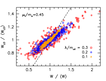
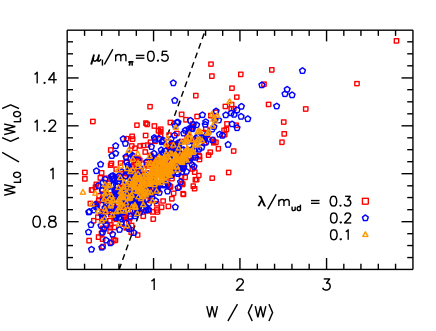
Thus we conclude that the reweighting of an observable, to leading order in , involves the exponential of the pion condensate (measured at ) times the four-volume. Since the pion condensate is anyway measured on the individual configurations to compute , this improvement comes with no extra costs. We test this improvement on small lattices, where a calculation of the complete spectrum of singular values is feasible, enabling a direct comparison between and . Specifically, we employ the low-temperature ensembles generated in Ref. Endrődi (2014) and plot the two reweighting factors against each other in Fig. 3 for two values of around the critical isospin chemical potential. The scatter plot clearly shows the strong correlation between and and that the two factors become identical in the limit .444Notice furthermore that tends to overestimate if the reweighting factors are below average (and vice versa). This can be understood using the singular value representation of Eqs. (25) and (26), (27) which can be used to show that the difference is a positive and monotonously decreasing function of at fixed . Thus, a fluctuation that reduces the singular values (i.e. that pushes below average), inevitably increases the deviation , thereby explaining the tendency visible in Fig. 3.
IV Results: improvement program
In the following we always perform the leading order reweighting with , where is calculated from (13) employing noisy estimators to evaluate the traces. The measurements are carried out on the reweighted ensembles.
IV.1 Improved pion condensate
We describe our strategy to determine in more detail. The singular values of the massive Dirac operator (i.e., the eigenvalues of , cf. Eq. (20)) are calculated using the Krylov-Schur algorithm. We find it sufficient to work with the lowest 50-150 singular values for each configuration. Using this set of singular values we build a histogram for the integrated spectral density
| (28) |
where we discard bins that lie below the average lowest singular value. The statistical error of in each bin is estimated via the jackknife procedure. In Fig. 4 we plot for two ensembles just around and slightly beyond the transition to the pion condensed phase.
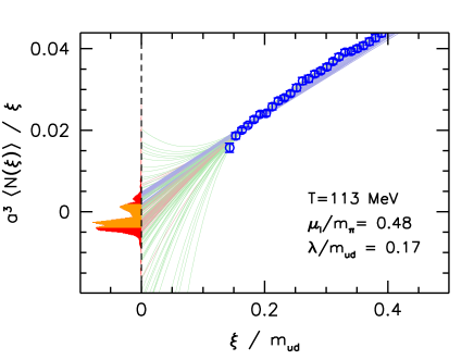
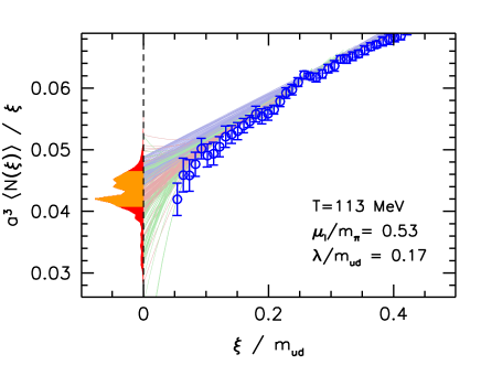
To obtain , we need to extrapolate down to zero. This is performed via polynomial fits of the histogram. To take into account the correlation between the individual bins, we minimize the correlated , which involves the inverse of the correlation matrix of the data. To avoid numerical problems during this inversion, we smear the lowest eigenvalues of following the strategy of Ref. Michael and McKerrell (1995). We perform the fits with polynomials of various degrees and over various fit ranges. The resulting values for are weighted by with the number of degrees of freedom in the fit. The weighted results are used to build yet another histogram (red area in Fig. 4), similar to the analysis conducted in Ref. Borsányi et al. (2015). The central value for is obtained by the median, while the statistical plus systematical error of the fit is estimated by the range that contains the middle of the histogram (orange area in Fig. 4). The analysis gives drastically different results for the two chemical potentials considered in the figure. While the intersect of the fits is large for , it is consistent with zero for . (In the latter case and its error is taken as the positive part of the orange histogram.) This demonstrates – via the relation (21) – the emergence of a nonzero pion condensate in the BEC phase. The so obtained results for are included in the top panel of Fig. 2 above.
IV.2 Improved quark condensate
In principle, for the improvement scheme of the quark condensate, outlined in Sec. III.3, we need all singular values . This is in contrast to the improvement of the pion condensate, where only the spectral density of singular values around zero is of importance. Nevertheless, computing all singular values for each configuration is unfeasible in practice and, in fact, not necessary. The important simplification follows from the observation that the difference from Eq. (24) is dominated by the dependence of the terms involving the lowest singular values. It might thus be sufficient to perform the explicit extrapolation in the operator for only the first low modes and to leave the contribution from the remaining singular values untouched. To this end we introduce the truncated operator
| (29) |
and the associated truncated difference
| (30) |
to rewrite the expectation value as
| (31) |
The second term vanishes when we perform the -extrapolation, so that we obtain
| (32) |
This type of improvement will be efficient if is large enough to ensure that so that the subtraction effectively removes most of the dependence of the observable.
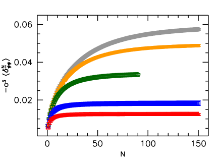
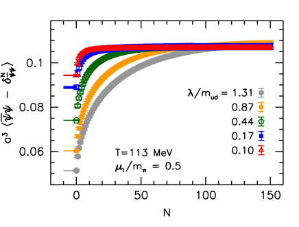
The optimal value for to achieve a good balance between the improvement for the dependence of the observable and the computational cost will, in general, depend on the operator, the lattice size and the lattice spacing, as well as on the magnitude of the -values in use. The results for versus for different values of are shown in the top panel of Fig. 5. The figure indicates that moderate values of suffice to ensure that most of the dependence in the valence sector is absorbed by the improvement. In the bottom panel of Fig. 5 we plot the combination , revealing no significant dependence for . For comparison, the dependence of the unimproved observable (marked by the short horizontal lines in the figure) is much more pronounced.
We find that does suffice to warrant well controlled -extrapolations for all ensembles and observables considered so far. Thus, the same set of singular values can be used for the improvement of the pion condensate as well as for the quark condensate.
IV.3 Final -extrapolations
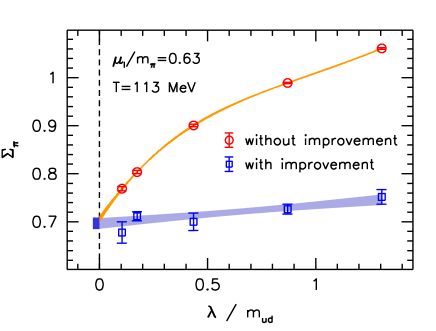
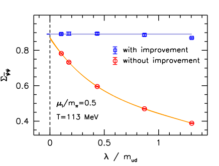
Having performed the improvements described above, we can carry out the final extrapolation of the results to . Since the improvements do not achieve a perfect elimination of the pionic source [the reweighting is done only at leading order, the singular value sums are truncated at a finite , and the finiteness of the volume distorts the relation (21)], a mild dependence of the results on is still expected. In Fig. 6 we show a few representative examples for the extrapolations of and of , where we also include the unimproved observables [i.e. the quantities obtained via the full traces, Eq. (13)]. Contrary to the pronounced (and thus uncontrolled) dependence of the latter on , we find that the improved observables can be reliably fitted by either a constant or a linear function (on general grounds, is an odd function of , whereas is even in the pionic source). We also attempted to perform a fit of the unimproved data by means of a spline with Monte-Carlo-generated nodepoints (for the details of this fit procedure, see Ref. Brandt and Endrődi (2016)). For comparison, the so obtained extrapolations are also included in Fig. 6. Unlike the improved extrapolations, these fits are always dominated by the points at low , making them unreliable in several cases.
V Results
V.1 Phase diagram
In the following we work with the extrapolated observables to determine the phase diagram of the system in the plane. We work with four lattice ensembles with , , and . Fig. 7 shows our results for and for from Eq. (15). The onset of pion condensation is characterized by the abrupt change at the boundary between the vacuum and the BEC phase, mapping a critical line . The quark condensate exhibits a similarly pronounced change at the pion condensation phase boundary. In addition, it also features a smooth dependence on the temperature around the chiral crossover transition . In the following, we refer to the point, where these two transition lines meet as the pseudo-triple point at and . The notation refers to the fact that the chiral transition is pseudocritical and does not correspond to a true phase transition (in which case this point would be a true triple point).
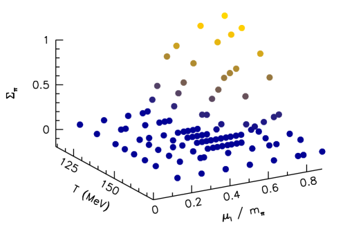
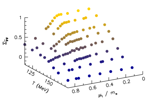
The boundary of the pion condensation phase, , is determined by the points where acquires a nonzero expectation value. We estimate its location by interpolating555A technical issue regarding this fit is the non-analyticity of at the critical chemical potential. Although it is regulated by the finite volume, the sharp behavior around cannot be captured by the smooth splines. To avoid this issue, here we fit the results from Sec. IV.1, allowing for negative intersects for (i.e. the full orange histograms of Fig. 4). This enables a more stable determination of the contour. the results for using a two-dimensional cubic spline fit with Monte-Carlo-generated nodepoints Brandt and Endrődi (2016). From PT it is known that Son and Stephanov (2001). We observe that is independent of up to a temperature of about to MeV – see also the results shown in Brandt and Endrődi (2016); Brandt et al. (2017). For a temperature of about to MeV the phase boundary starts to flatten out, and above MeV the pion condensate is found to vanish within errors for all ensembles. Here we follow the phase boundary up to MeV, but this flat behavior is found to persist at least up to MeV on our ensemble, see below. These findings contradict the expectations from PT, which predicts a monotonous rise in Son and Stephanov (2001).
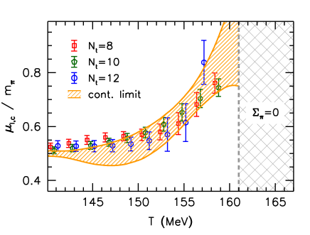
To perform the continuum extrapolation, we parameterize by a polynomial in with lattice spacing dependent coefficients. We set MeV, below which is found to be independent of . To capture both the flatness of the critical chemical potential for low temperatures and its abrupt rise around , we found it necessary to include terms proportional to , and in the fit and to fix . We find that for , our results are outside of the scaling region for lattice artefacts of so that we excluded these from the continuum extrapolation. The final continuum curve, extrapolated including terms proportional to , is shown in Fig. 8 (top panel), together with the data for the phase boundary which has been included in the fit. MeV serves as an upper bound for the critical temperature, as is found to vanish within the uncertainties for all lattice spacings and for all values of considered in this region, as mentioned above.
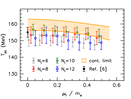
We proceed with the chiral crossover transition temperature , which we define as the location of the inflection point of with respect to .666Note that in Refs. Brandt and Endrődi (2016); Brandt et al. (2017) we employed a different procedure, defining as the point where holds. This definition is only valid for , since beyond that the condensate is affected by already at . On the contrary, the inflection point can be used to define at any value of . The data shows an initial reduction in up to about , followed by a slight increase. Beyond the pseudo-triple point, where the crossover line and the pion condensation boundary meet, we observe the two transition lines to coincide within errors. To be more quantitative, we once again determine using a two-dimensional spline fit where the nodepoints have been generated via Monte-Carlo. In the spline fit777 Here we only take into account the fit for , where the spline captures the behavior of sufficiently accurately. Below this temperature the condensate changes abruptly at the BEC phase transition, which is not captured by our smooth interpolation. we include the constraint that is an even function of . To perform the continuum extrapolation, we parameterize by a polynomial which is even in , including data up to . The behavior of beyond this value is difficult to capture with polynomials. For the range of chemical potentials included in the fit, the data is already well described by a quadratic polynomial in and lattice artefacts, see Fig. 8 (bottom panel). Adding a -term or higher-order lattice discretization errors was found to only increase the uncertainties and not lead to significant differences.
The precise location of the pseudo-triple point is also of interest. We define to be the value for where the two transition lines become consistent within errors – i.e. where the uncertainties overlap. This provides a conservative lower bound for the pseudo-triple point. The results for are shown in Fig. 9. As for the pion condensation phase boundary, the continuum extrapolation is performed including lattice artefacts of and excluding the results. The resulting continuum extrapolation is indicated by the shaded orange band in Fig. 9. We found this extrapolation to be more stable than the fit to all available lattice spacings, including lattice artefacts of . Both extrapolations lead to similar results, see the comparison in Fig. 9.
We are now in the position to draw the continuum phase diagram, which we display in Fig. 10. The chiral crossover transition starts from a temperature of MeV, which is consistent with the crossover temperatures from Borsányi et al. (2010); *Bazavov:2011nk within uncertainties. The results exhibit a small downward curvature of the line. The pion condensation boundary remains at within our errors up to , beyond which it soon becomes very flat. For MeV, we do not observe pion condensation up to MeV.
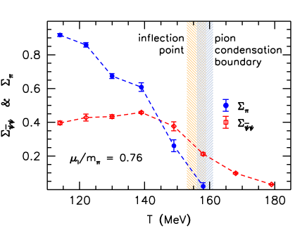
The two transition lines meet at the pseudo-triple point, for which we obtain MeV in the continuum limit, indicated by the yellow point in Fig. 10. The corresponding temperature is determined conservatively by taking into account the upper bound for and the lower bound for the temperature where . Defining the central value of as the midpoint of this interval we obtain MeV. From what we observe at finite lattice spacings, we expect that chiral symmetry restoration and the pion condensation phase boundary coincide from the pseudo-triple point on. To demonstrate this, in Fig. 11 we plot the pion condensate together with the quark condensate for . The figure indicates that pion condensation (defined by the point where ) occurs together with chiral symmetry restoration (the inflection point of the condensate). The initial rise of the chiral condensate in Fig. 11 is an interesting feature in the pion condensation phase. A similar tendency has been observed in a study of the phase diagram of a related two-color NJL model Ratti and Weise (2004). We interpret it as a remnant of the relation between pion and chiral condensate , discussed in Sec. II.3, which follows from PT to leading order Son and Stephanov (2001).
V.2 Polyakov loop
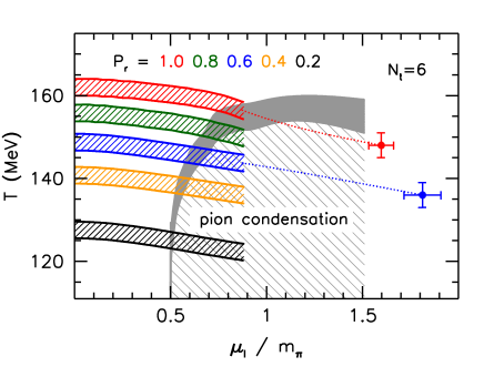
Next, we elaborate on the properties of the deconfinement transition in terms of the renormalized Polyakov loop . In contrast to the quark condensate, the Polyakov loop exhibits no pronounced inflection point. To capture how deconfinement depends on the isospin chemical potential, we consider the curves in the plane, where is satisfied. Considering our definition (17) for the renormalization, the contour with is a possible choice for the transition temperature. In addition, the distance between the various contour lines is related to the slope of around the transition point. We show the contours of constant in the phase diagram for in Fig. 12. The contour lines are observed to be insensitive to the BEC phase transition, as they enter the pion condensation phase without any sign of critical behavior. In this plot we also included results obtained at high isospin chemical potentials, up to for the pion condensation boundary and up to for a few Polyakov loop contours. After crossing the phase boundary, the contours continue to decrease, in agreement with the sketch of the phase diagram in Fig. 1. We postpone a more detailed discussion of the deconfinement transition to a future publication with an extended range in .
V.3 Order of the BEC transition
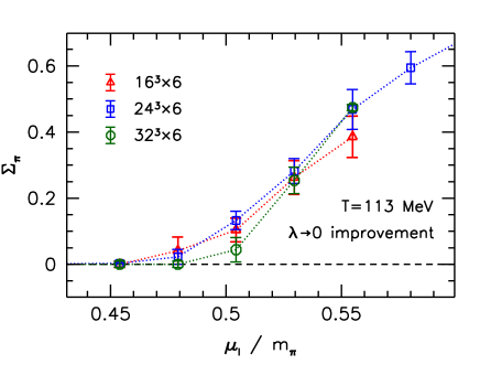
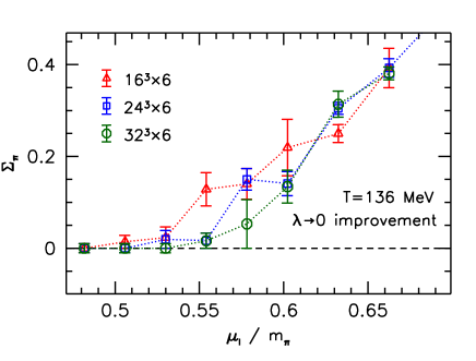
Finally, we investigate the nature of the transition between the vacuum and the pion condensed phase via a finite size scaling analysis. To this end three ensembles with , and are employed. The results for around the critical isospin chemical potential are shown in Fig. 13. Both at and at a sharpening of is visible, confirming that a real phase transition takes place in the limit. To be more quantitative, we proceed with the assumption that the transition is of second order. In this case, our results at and must reflect the critical behavior that emerges as and in the vicinity of the transition point. For the following analysis we use the data obtained on the ensemble at the lowest temperature .
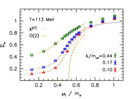
First we compare our (unimproved) results for to the prediction of PT. This involves two free parameters: the critical isospin chemical potential and a normalization factor , which corresponds to the magnitude of the renormalized quark condensate in the vacuum,
| (33) |
where the vacuum angle is determined implicitly by the second equation (see Refs. Splittorff et al. (2002); Endrődi (2014)). The data is very well described by the predicted behavior, see the top panel of Fig. 14. Taking into account data points for and the two smallest pionic sources , we obtain a reasonable fit with . For higher isospin chemical potentials PT tends to underestimate , as has already been noted in Ref. Endrődi (2014). The critical chemical potential is and the normalization factor , both very close to the values expected in the zero-temperature and thermodynamic limits ( and unity, respectively).
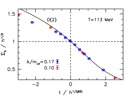
We also consider the critical behavior of the universality class to fit the order parameter as a function of and . In particular, this dependence involves the universal scaling function ,
| (34) |
with the critical exponents and and the free parameters , , and . For the construction of , we follow Ref. Ejiri et al. (2009). The result of the fit, using the two lowest pionic sources and isospin chemical potentials , is shown in the bottom panel of Fig. 14, demonstrating the collapse of the data on the universal curve. The critical chemical potential is found to be . However, since the fit quality is rather low (), we extended the fit function to include scaling violations in the spirit of Ref. Ejiri et al. (2009). We found it necessary to work with
| (35) |
which allowed us to achieve reasonable fit qualities () for broader fit intervals and . The resulting fit is included in the top panel of Fig. 14. We find , again lying very close to the expected value of .
Summarizing, our results strongly indicate that the transition into the pion condensed phase is of second order in the infinite volume limit. In addition, the behavior of the order parameter at nonzero values of the explicit breaking parameter is consistent with the critical scaling in the universality class, as expected due to the spontaneous symmetry breaking pattern discussed in Sec. II.1.
VI Summary
In this paper we have presented the first study of the phase diagram of QCD at nonzero isospin chemical potentials in the continuum limit with dynamical , and quarks at physical quark masses. Our main result is the continuum extrapolated phase diagram, as shown in Fig. 10. The key features of the phase diagram are the chiral crossover transition, the pion condensation boundary and their meeting point, the pseudo-triple point. We observe that the critical chemical potential for pion condensation remains constant up to MeV, followed by a drastic change in behavior and a saturation at around MeV. Above this temperature, we no longer observe pion condensation, at least up to MeV. This finding might be particularly relevant for the orbifold equivalence in the large limit, as the pion condensation region is smaller than previously expected.
The chiral crossover temperature decreases slightly until it reaches the vicinity of the pion condensation phase boundary. The two transition lines meet at MeV and are found to be on top of each other within uncertainties for higher isospin chemical potentials. Our scaling analysis of the pion condensation boundary shows consistency with a second order phase transition in the universality class.
Using our lattice ensembles, we find first indications that the deconfinement transition temperature – defined in terms of the renormalized Polyakov loop – decreases and smoothly penetrates into the pion condensation phase. This behavior is depicted schematically in Fig. 1. If this tendency persists in the continuum limit and for larger values of , the scenario where the deconfinement transition connects continuously to the BEC-BCS crossover will be favored. Our results for the phase diagram can be compared directly to effective theories and models of QCD and serve as a highly nontrivial check of the validity of these approaches.
The main technical novelty of this study is the development of an improvement program for the extrapolations in the infrared regulator , discussed in detail in Secs. III and IV. Without the use of these improved extrapolations the reliable extraction of the phase diagram would have hardly been possible. We would like to emphasize that a similar infrared regulator will likely be necessary to enable simulations at finite baryon chemical potential – granted that the sign problem has been solved. In this case, a generalization of the methods presented here might be helpful to give insight to the investigations at finite .
Acknowledgements.
This research was funded by the DFG (Emmy Noether Programme EN 1064/2-1 and SFB/TRR 55). The simulations were performed on the GPU cluster of the Institute for Theoretical Physics at the University of Regensburg and on the FUCHS and LOEWE clusters at the Center for Scientific Computing of the Goethe University of Frankfurt. The authors thank Gunnar Bali, Falk Bruckmann, Tom DeGrand, Simon Hands, Sándor Katz, Andreas Schäfer, Lorenz von Smekal, Kálmán Szabó and Tilo Wettig for illuminating discussions.References
- Li et al. (1998) B.-A. Li, C. M. Ko, and W. Bauer, Int. J. Mod. Phys. E7, 147 (1998), arXiv:nucl-th/9707014 [nucl-th] .
- Steiner et al. (2005) A. W. Steiner, M. Prakash, J. M. Lattimer, and P. J. Ellis, Phys. Rept. 411, 325 (2005), arXiv:nucl-th/0410066 [nucl-th] .
- Migdal et al. (1990) A. B. Migdal, E. Saperstein, M. Troitsky, and D. Voskresensky, Phys.Rept. 192, 179 (1990).
- Schwarz and Stuke (2009) D. J. Schwarz and M. Stuke, JCAP 0911, 025 (2009), [Erratum: JCAP1010,E01(2010)], arXiv:0906.3434 [hep-ph] .
- Aoki et al. (2006a) Y. Aoki, G. Endrődi, Z. Fodor, S. D. Katz, and K. K. Szabó, Nature 443, 675 (2006a), arXiv:hep-lat/0611014 [hep-lat] .
- Bhattacharya et al. (2014) T. Bhattacharya et al., Phys. Rev. Lett. 113, 082001 (2014), arXiv:1402.5175 [hep-lat] .
- Borsányi et al. (2010) S. Borsányi, Z. Fodor, C. Hoelbling, S. D. Katz, S. Krieg, C. Ratti, and K. K. Szabó (Wuppertal-Budapest), JHEP 09, 073 (2010), arXiv:1005.3508 [hep-lat] .
- Bazavov et al. (2012) A. Bazavov et al., Phys. Rev. D85, 054503 (2012), arXiv:1111.1710 [hep-lat] .
- Son and Stephanov (2001) D. T. Son and M. A. Stephanov, Phys. Rev. Lett. 86, 592 (2001), arXiv:hep-ph/0005225 [hep-ph] .
- Brandt and Endrődi (2016) B. B. Brandt and G. Endrődi, Proceedings, 34th International Symposium on Lattice Field Theory (Lattice 2016): Southampton, UK, July 24-30, 2016, PoS LATTICE2016, 039 (2016), arXiv:1611.06758 [hep-lat] .
- Brandt et al. (2017) B. B. Brandt, G. Endrődi, and S. Schmalzbauer, in 35th International Symposium on Lattice Field Theory (Lattice 2017) Granada, Spain, June 18-24, 2017 (2017) arXiv:1709.10487 [hep-lat] .
- Cohen and Sen (2015) T. D. Cohen and S. Sen, Nucl. Phys. A942, 39 (2015), arXiv:1503.00006 [hep-ph] .
- Splittorff et al. (2001) K. Splittorff, D. T. Son, and M. A. Stephanov, Phys. Rev. D64, 016003 (2001), arXiv:hep-ph/0012274 [hep-ph] .
- Loewe and Villavicencio (2003) M. Loewe and C. Villavicencio, Phys. Rev. D67, 074034 (2003), arXiv:hep-ph/0212275 [hep-ph] .
- Fraga et al. (2009) E. S. Fraga, L. F. Palhares, and C. Villavicencio, Phys. Rev. D79, 014021 (2009), arXiv:0810.1060 [hep-ph] .
- Janssen et al. (2016) O. Janssen, M. Kieburg, K. Splittorff, J. J. M. Verbaarschot, and S. Zafeiropoulos, Phys. Rev. D93, 094502 (2016), arXiv:1509.02760 [hep-lat] .
- Carignano et al. (2017) S. Carignano, L. Lepori, A. Mammarella, M. Mannarelli, and G. Pagliaroli, Eur. Phys. J. A53, 35 (2017), arXiv:1610.06097 [hep-ph] .
- Andersen et al. (2016) J. O. Andersen, N. Haque, M. G. Mustafa, and M. Strickland, Phys. Rev. D93, 054045 (2016), arXiv:1511.04660 [hep-ph] .
- Toublan and Kogut (2003) D. Toublan and J. B. Kogut, Phys. Lett. B564, 212 (2003), arXiv:hep-ph/0301183 [hep-ph] .
- Frank et al. (2003) M. Frank, M. Buballa, and M. Oertel, Phys. Lett. B562, 221 (2003), arXiv:hep-ph/0303109 [hep-ph] .
- Barducci et al. (2004) A. Barducci, R. Casalbuoni, G. Pettini, and L. Ravagli, Phys. Rev. D69, 096004 (2004), arXiv:hep-ph/0402104 [hep-ph] .
- He and Zhuang (2005) L. He and P. Zhuang, Phys. Lett. B615, 93 (2005), arXiv:hep-ph/0501024 [hep-ph] .
- Zhang and Liu (2007a) Z. Zhang and Y.-X. Liu, Phys. Rev. C75, 064910 (2007a), arXiv:hep-ph/0610221 [hep-ph] .
- Sun et al. (2007) G.-f. Sun, L. He, and P. Zhuang, Phys. Rev. D75, 096004 (2007), arXiv:hep-ph/0703159 [hep-ph] .
- Xia et al. (2013) T. Xia, L. He, and P. Zhuang, Phys. Rev. D88, 056013 (2013), arXiv:1307.4622 [hep-ph] .
- Zhang and Miao (2016) Z. Zhang and Q. Miao, Phys. Lett. B753, 670 (2016), arXiv:1507.07224 [hep-ph] .
- Brauner and Huang (2016) T. Brauner and X.-G. Huang, Phys. Rev. D94, 094003 (2016), arXiv:1610.00426 [hep-ph] .
- Khunjua et al. (2017) T. G. Khunjua, K. G. Klimenko, and R. N. Zhokhov, (2017), arXiv:1710.09706 [hep-ph] .
- Gubina et al. (2012) N. V. Gubina, K. G. Klimenko, S. G. Kurbanov, and V. C. Zhukovsky, Phys. Rev. D86, 085011 (2012), arXiv:1206.2519 [hep-ph] .
- He et al. (2005) L.-y. He, M. Jin, and P.-f. Zhuang, Phys. Rev. D71, 116001 (2005), arXiv:hep-ph/0503272 [hep-ph] .
- Ueda et al. (2013) H. Ueda, T. Z. Nakano, A. Ohnishi, M. Ruggieri, and K. Sumiyoshi, Phys. Rev. D88, 074006 (2013), arXiv:1304.4331 [nucl-th] .
- Stiele et al. (2014) R. Stiele, E. S. Fraga, and J. Schaffner-Bielich, Phys. Lett. B729, 72 (2014), arXiv:1307.2851 [hep-ph] .
- Andersen (2007) J. O. Andersen, Phys. Rev. D75, 065011 (2007), arXiv:hep-ph/0609020 [hep-ph] .
- Klein et al. (2003) B. Klein, D. Toublan, and J. J. M. Verbaarschot, Phys. Rev. D68, 014009 (2003), arXiv:hep-ph/0301143 [hep-ph] .
- Klahn et al. (2017) T. Klahn, T. Fischer, and M. Hempel, Astrophys. J. 836, 89 (2017), arXiv:1603.03679 [nucl-th] .
- Toublan and Kogut (2005) D. Toublan and J. B. Kogut, Phys. Lett. B605, 129 (2005), arXiv:hep-ph/0409310 [hep-ph] .
- Zhang and Liu (2007b) Z. Zhang and Y.-x. Liu, Phys. Rev. C75, 035201 (2007b), arXiv:hep-ph/0603252 [hep-ph] .
- Svanes and Andersen (2011) E. E. Svanes and J. O. Andersen, Nucl. Phys. A857, 16 (2011), arXiv:1009.0430 [hep-ph] .
- Kamikado et al. (2013) K. Kamikado, N. Strodthoff, L. von Smekal, and J. Wambach, Phys. Lett. B718, 1044 (2013), arXiv:1207.0400 [hep-ph] .
- Wang and Zhuang (2017) Z. Wang and P. Zhuang, Phys. Rev. D96, 014006 (2017), arXiv:1703.01035 [hep-ph] .
- Kashiwa and Ohnishi (2017) K. Kashiwa and A. Ohnishi, Phys. Lett. B772, 669 (2017), arXiv:1701.04953 [hep-ph] .
- Aharony et al. (2008) O. Aharony, K. Peeters, J. Sonnenschein, and M. Zamaklar, JHEP 02, 071 (2008), arXiv:0709.3948 [hep-th] .
- Basu et al. (2009) P. Basu, J. He, A. Mukherjee, and H.-H. Shieh, JHEP 11, 070 (2009), arXiv:0810.3970 [hep-th] .
- Albrecht and Erlich (2010) D. Albrecht and J. Erlich, Phys. Rev. D82, 095002 (2010), arXiv:1007.3431 [hep-ph] .
- Hanada and Yamamoto (2012) M. Hanada and N. Yamamoto, JHEP 02, 138 (2012), arXiv:1103.5480 [hep-ph] .
- Kogut and Sinclair (2002a) J. B. Kogut and D. K. Sinclair, Phys. Rev. D66, 014508 (2002a), arXiv:hep-lat/0201017 [hep-lat] .
- Kogut and Sinclair (2002b) J. B. Kogut and D. K. Sinclair, Phys. Rev. D66, 034505 (2002b), arXiv:hep-lat/0202028 [hep-lat] .
- Kogut and Sinclair (2004) J. B. Kogut and D. K. Sinclair, Phys. Rev. D70, 094501 (2004), arXiv:hep-lat/0407027 [hep-lat] .
- Cea et al. (2012) P. Cea, L. Cosmai, M. D’Elia, A. Papa, and F. Sanfilippo, Phys. Rev. D85, 094512 (2012), arXiv:1202.5700 [hep-lat] .
- Endrődi (2014) G. Endrődi, Phys. Rev. D90, 094501 (2014), arXiv:1407.1216 [hep-lat] .
- de Forcrand et al. (2007) P. de Forcrand, M. A. Stephanov, and U. Wenger, Proceedings, 25th International Symposium on Lattice field theory (Lattice 2007): Regensburg, Germany, July 30-August 4, 2007, PoS LAT2007, 237 (2007), arXiv:0711.0023 [hep-lat] .
- Detmold et al. (2012) W. Detmold, K. Orginos, and Z. Shi, Phys. Rev. D86, 054507 (2012), arXiv:1205.4224 [hep-lat] .
- Allton et al. (2005) C. R. Allton, M. Doring, S. Ejiri, S. J. Hands, O. Kaczmarek, F. Karsch, E. Laermann, and K. Redlich, Phys. Rev. D71, 054508 (2005), arXiv:hep-lat/0501030 [hep-lat] .
- Borsányi et al. (2012a) S. Borsányi, Z. Fodor, S. D. Katz, S. Krieg, C. Ratti, and K. Szabó, JHEP 01, 138 (2012a), arXiv:1112.4416 [hep-lat] .
- Nishida (2004) Y. Nishida, Phys. Rev. D69, 094501 (2004), arXiv:hep-ph/0312371 [hep-ph] .
- Langelage et al. (2014) J. Langelage, M. Neuman, and O. Philipsen, JHEP 09, 131 (2014), arXiv:1403.4162 [hep-lat] .
- Kogut et al. (2001) J. B. Kogut, D. K. Sinclair, S. J. Hands, and S. E. Morrison, Phys. Rev. D64, 094505 (2001), arXiv:hep-lat/0105026 [hep-lat] .
- Hands et al. (2006) S. Hands, S. Kim, and J.-I. Skullerud, Eur. Phys. J. C48, 193 (2006), arXiv:hep-lat/0604004 [hep-lat] .
- Bornyakov et al. (2017) V. G. Bornyakov, V. V. Braguta, E. M. Ilgenfritz, A. Yu. Kotov, A. V. Molochkov, and A. A. Nikolaev, (2017), arXiv:1711.01869 [hep-lat] .
- Andersen and Brauner (2010) J. O. Andersen and T. Brauner, Phys. Rev. D81, 096004 (2010), arXiv:1001.5168 [hep-ph] .
- Strodthoff et al. (2012) N. Strodthoff, B.-J. Schaefer, and L. von Smekal, Phys. Rev. D85, 074007 (2012), arXiv:1112.5401 [hep-ph] .
- von Smekal (2012) L. von Smekal, Physics at all scales: The Renormalization Group. Proceedings, 49. Internationale Universitätswochen für Theoretische Physik, Winter School: Schladming, Austria, February 26-March 5, 2011, Nucl. Phys. Proc. Suppl. 228, 179 (2012), arXiv:1205.4205 [hep-ph] .
- Cohen (2003) T. D. Cohen, Phys. Rev. Lett. 91, 222001 (2003), arXiv:hep-ph/0307089 [hep-ph] .
- Bali et al. (2016) G. S. Bali, G. Endrődi, R. V. Gavai, and N. Mathur (2016) arXiv:1610.00233 [hep-lat] .
- Frezzotti et al. (2001) R. Frezzotti, P. A. Grassi, S. Sint, and P. Weisz (Alpha), JHEP 08, 058 (2001), arXiv:hep-lat/0101001 [hep-lat] .
- Dürr (2006) S. Dürr, Proceedings, 23rd International Symposium on Lattice field theory (Lattice 2005): Dublin, Ireland, Jul 25-30, 2005, PoS LAT2005, 021 (2006), arXiv:hep-lat/0509026 [hep-lat] .
- Borsányi et al. (2010) S. Borsányi et al., JHEP 11, 077 (2010), arXiv:1007.2580 [hep-lat] .
- Aoki et al. (2006b) Y. Aoki, Z. Fodor, S. D. Katz, and K. K. Szabó, JHEP 01, 089 (2006b), arXiv:hep-lat/0510084 [hep-lat] .
- Urbach et al. (2006) C. Urbach, K. Jansen, A. Shindler, and U. Wenger, Comput. Phys. Commun. 174, 87 (2006), arXiv:hep-lat/0506011 [hep-lat] .
- Leutwyler and Smilga (1992) H. Leutwyler and A. V. Smilga, Phys. Rev. D46, 5607 (1992).
- Hasenfratz and Karsch (1983) P. Hasenfratz and F. Karsch, Phys. Lett. 125B, 308 (1983).
- Bali et al. (2012) G. S. Bali, F. Bruckmann, G. Endrődi, Z. Fodor, S. D. Katz, and A. Schäfer, Phys. Rev. D86, 071502 (2012), arXiv:1206.4205 [hep-lat] .
- Borsányi et al. (2012b) S. Borsányi, S. Dürr, Z. Fodor, C. Hoelbling, S. D. Katz, S. Krieg, D. Nográdi, K. K. Szabó, B. C. Tóth, and N. Trombitás, JHEP 08, 126 (2012b), arXiv:1205.0440 [hep-lat] .
- Bruckmann et al. (2013) F. Bruckmann, G. Endrődi, and T. G. Kovács, JHEP 04, 112 (2013), arXiv:1303.3972 [hep-lat] .
- Kanazawa et al. (2011) T. Kanazawa, T. Wettig, and N. Yamamoto, JHEP 12, 007 (2011), arXiv:1110.5858 [hep-ph] .
- Banks and Casher (1980) T. Banks and A. Casher, Nucl. Phys. B169, 103 (1980).
- Michael and McKerrell (1995) C. Michael and A. McKerrell, Phys. Rev. D51, 3745 (1995), arXiv:hep-lat/9412087 [hep-lat] .
- Borsányi et al. (2015) S. Borsányi et al., Science 347, 1452 (2015), arXiv:1406.4088 [hep-lat] .
- Ratti and Weise (2004) C. Ratti and W. Weise, Phys. Rev. D70, 054013 (2004), arXiv:hep-ph/0406159 [hep-ph] .
- Splittorff et al. (2002) K. Splittorff, D. Toublan, and J. J. M. Verbaarschot, Nucl. Phys. B639, 524 (2002), arXiv:hep-ph/0204076 [hep-ph] .
- Ejiri et al. (2009) S. Ejiri, F. Karsch, E. Laermann, C. Miao, S. Mukherjee, P. Petreczky, C. Schmidt, W. Soeldner, and W. Unger, Phys. Rev. D80, 094505 (2009), arXiv:0909.5122 [hep-lat] .