Adjacency and Tensor Representation in General Hypergraphs
Part 1: e-adjacency Tensor Uniformisation Using Homogeneous Polynomials

Abstract

Adjacency between two vertices in graphs or hypergraphs is a pairwise relationship. It is redefined in this article as 2-adjacency. In general hypergraphs, hyperedges hold for $n$-adic relationship. To keep the $n$-adic relationship the concepts of k-adjacency and e-adjacency are defined. In graphs 2-adjacency and e-adjacency concepts match, just as $k$-adjacency and e-adjacency do for $k$-uniform hypergraphs. For general hypergraphs these concepts are different. This paper also contributes in a uniformization process of a general hypergraph to allow the definition of an e-adjacency tensor, viewed as a hypermatrix, reflecting the general hypergraph structure. This symmetric e-adjacency hypermatrix allows to capture not only the degree of the vertices and the cardinality of the hyperedges but also makes a full separation of the different layers of a hypergraph.

1 Introduction

Hypergraphs were introduced in 1973 Berge and Minieka (1973). Hypergraphs have applications in many domains such as VLSI design, biology or collaboration networks. Edges of a graph allow to connect only two vertices where hyperedges of hypergraphs allow multiple vertices to be connected. Recent improvements in tensor spectral theory have made the research on the spectra of hypergraphs more relevant. For studying such spectra a proper definition of general hypergraph Laplacian tensor is needed and therefore the concept of adjacency has to be clearly defined and consequently an (-as it will be defined later- e-)adjacency tensor must be properly defined.

In Pu (2013) a clear distinction is made between the pairwise relationship which is a binary relation and the co-occurrence relationship which is presented as the extension of the pairwise relationship to a $p$-adic relationship. The notion of co-occurrence is often used in linguistic data as the simultaneous appearance of linguistic units in a reference. The co-occurence concept can be easily extended to vertices contained in a hyperedge: we designate it in hypergraphs by the term e-adjacency.

Nonetheless it is more than an extension. Graph edges allow to connect vertices by pair: graph adjacency concept is clearly a pairwise relationship. At the same time in an edge only two vertices are linked. Also given an edge only two vertices can be e-adjacent. Thus adjacency and e-adjacency are equivalent in graphs.

Extending to hypergraphs the adjacency notion two vertices are said adjacent if it exists a hyperedge that connect them. Hence the adjacency notion still captures a binary relationship and can be modeled by an adjacency matrix. But e-adjacency is no more a pairwise relationship as a hyperedge being given more than two vertices can occur since a hyperedge contains $p\geqslant 1$ vertices. Therefore it is a $p$-adic relationship that has to be captured and to be modeled by tensor. Consequently adjacency matrix of a hypergraph and e-adjacency tensor are two separated notions. Nonetheless the e-adjacency tensor if often abusively named the adjacency tensor in the literature.

This article contributions are: 1. the definition of proper adjacency concept in general hypergraphs; 2. a process to achieve the transformation of a general hypergraph into a uniform hypergraph called uniformization process; 3. the definition of a new (e-)adjacency tensor which not solely preserves all the structural information of the hypergraph but also captures separately the information on the hyperedges held in the hypergraph.

After sketching the background and the related works on the adjacency and e-adjacency concepts for hypergraphs in Section 2, one proposal is made to build a new e-adjacency tensor which is built as unnormalized in Section 3. Section 4 tackles the particular case of graphs seen as 2-uniform hypergraphs and the link with DNF. Future works and Conclusion are addressed in Section 6. A full example is given in Appendix A.

Notation

Exponents are indicated into parenthesis - for instance $y^{(n)}$ - when they refer to the order of the corresponding tensor. Indices are written into parenthesis when they refer of a sequence of objects - for instance $a_{(k)ij}$ is the elements at row $i$ and column $j$ of the matrix $A_{(k)}$ -. The context should made it clear.

For the convenience of readability, it is written $\boldsymbol{z}_{0}$ for $z^{1},...,z^{n}$. Hence given a polynomial $P$, $P\left(\boldsymbol{z}_{0}\right)$ has to be understood as $P\left(z^{1},...,z^{n}\right)$.

Given additional variables $y^{1},...,y^{k}$, it is written $\boldsymbol{z}_{k}$ for $z^{1},...,z^{n},y^{1},...,y^{k}$.

$\mathcal{S}_{k}$ is the set of permutations on the set $\left\{i\,:\,i\in\mathbb{N}\land 1\leqslant i\leqslant k\right\}$.

2 Background and related works

Several definitions of hypergraphs exist and are reminded in Ouvrard and Marchand-Maillet (2018). Hypergraphs allow the preservation of the $p$-adic relationship in between vertices becoming the natural modeling of collaboration networks, co-author networks, chemical reactions, genome and all situations where the 2-adic relationship allowed by graphs is not sufficient and where the keeping of the grouping information is important. Among the existing definitions the one of Bretto (2013) is reminded:

Definition 1.

An (undirected) hypergraph $\mathcal{H}=\left(V,E\right)$ on a finite set of $n$ vertices (or vertices) $V=\left\{v_{1}\,,\,v_{2},\,...\,,\,v_{n}\right\}$ is defined as a family of $p$ hyperedges $E=\left\{e_{1},e_{2},...,e_{p}\right\}$ where each hyperedge is a non-empty subset of $V$.

Let $\mathcal{H}=\left(V,E\right)$ be a hypergraph and $w$ a relation such that each hyperedge $e\in E$ is mapped to a real number $w(e)$. The hypergraph $\mathcal{H}_{w}=\left(V,E,w\right)$ is said to be a weighted hypergraph.

The $2$-section of a hypergraph $\mathcal{H}=\left(V,E\right)$ is the graph $\left[\mathcal{H}\right]_{2}=\left(V,E^{\prime}\right)$ such that:

$$\forall u\in V,\forall v\in V\,:\,(u,v)\in E^{\prime}\Leftrightarrow\exists e\in E\,:\,u\in e\land v\in e$$

Let $k\in\mathbb{N}^{*}$. a hypergraph is said to be $k-$uniform if all its hyperedges have the same cardinality $k$.

A directed hypergraph $\mathcal{H}=\left(V,E\right)$ on a finite set of $n$ vertices (or vertices) $V=\left\{v_{1}\,,\,v_{2},\,...\,,\,v_{n}\right\}$ is defined as a family of $p$ hyperedges $E=\left\{e_{1},e_{2},...,e_{p}\right\}$ where each hyperedge contains exactly two non-empty subset of $V$, one which is called the source - written $e_{s\,i}$ - and the other one which is the target - written $e_{t\,i}$ -.

In this article only undirected hypergraphs will be considered. In a hypergraph a hyperedge links one or more vertices together. The role of the hyperedges in hypergraphs is playing the role of edges in graphs.

Definition 2.

Let $\mathcal{H}=\left(V,E\right)$ be a hypergraph.

The degree of a vertex is the number of hyperedges it belongs to. For a vertex $v_{i}$, it is written $d_{i}$ or $\deg\left(v_{i}\right)$. It holds: $d_{i}=\left|\left\{e\,:\,v_{i}\in e\right\}\right|$

Given a hypergraph the incident matrix of an undirected hypergraph is defined as follow:

Definition 3.

The incidence matrix of a hypergraph is the rectangular matrix $H=\left[h_{kl}\right]_{\begin{subarray}{c}1\leqslant k\leqslant n\\ 1\leqslant l\leqslant p\end{subarray}}$ of $M_{n\times p}\left(\left\{0\,;\,1\right\}\right)$, where $h_{kl}=\begin{cases}1&\text{if\,}\,\,v_{k}\in e_{l}\\ 0&\text{otherwise}\end{cases}$.

As seen in the introduction defining adjacency in a hypergraph has to be distinguished from the e-adjacency in a hyperedge of a hypergraph.

Definition 4.

Let $\mathcal{H}=\left(V,E\right)$ be a hypergraph. Let $u\in V$ and $v\in V$ be two vertices of this hypergraph.

$u$ and $v$ are said adjacent if it exists $e\in E$ such that $u\in e$ and $v\in e$.

Definition 5.

Let $\mathcal{H}=\left(V,E\right)$ be a hypergraph. Let $k\geqslant 1$ be an integer, $j\in\left\llbracket 1;k\right\rrbracket$, $i_{j}\in\left\llbracket 1;n\right\rrbracket$. For $j\in\left\llbracket 1;k\right\rrbracket$, let $u_{i_{j}}\in V$ be $k$ vertices.

Then $u_{i_{1}}$,…,$u_{i_{k}}$ are said $k$-adjacent if it exists $e\in E$ such that for all $j\in\left\llbracket 1;k\right\rrbracket$, $u_{i_{j}}\in e$.

With $k=2$, the usual notion of adjacency is retrieved.

If $k$ vertices are $k$-adjacent then each subset of this $k$ vertices of size $l\leqslant k$ is $l$-adjacent.

Definition 6.

Let $\mathcal{H}=\left(V,E\right)$ be a hypergraph. Let $e\in E$.

The vertices constituting $e$ are said e-adjacent vertices.

If $\mathcal{H}$ is $k$-uniform then the $k$-adjacency is equivalent to the e-adjacency of vertices in an edge.

For a general hypergraph, vertices that are $k$-adjacent with $k<\underset{e\in E}{\max}\left|e\right|$ have to co-occur - potentially with other vertices - in one edge. In this case the notions of $k$-adjacency and of e-adjacency are actually distinct.

Adjacency matrix

The adjacency matrix of a hypergraph is related with the 2-adjacency. Several approaches have been made to define an adjacency matrix for hypergraphs.

In Bretto (2013) the adjacency matrix is defined as:

Definition 7.

The adjacency matrix is the square matrix which rows and columns are indexed by the vertices of $\mathcal{H}$ and where for all $u,v\in V$, $u\neq v$: $a_{uv}=\left|\left\{e\in E\,:\,u,v\in e\right\}\right|$ and $a_{uu}=0$.

The adjacency matrix is defined in Zhou et al. (2007) as follow:

Definition 8.

Let $\mathcal{H}_{w}=\left(V,E,w\right)$ be a weighted hypergraph.

The adjacency matrix of $\mathcal{H}_{w}$ is the matrix $A$ of size $n\times n$ defined as

$$A=HWH^{T}-D_{v}$$

where $W$ is the diagonal matrix of size $p\times p$ containing the weights of the hyperedges of $\mathcal{H}_{w}$ and $D_{v}$ is the diagonal matrix of size $n\times n$ containing the degrees of the vertices of $\mathcal{H}_{w}$, where $d(v)=\sum\limits_{\left\{e\in E\,:v\in e\right\}}w(e)$ for all $v\in V$.

This last definition is equivalent to the one of Bretto for unweighted hypergraphs - ie weighted hypergraphs where the weight of all hyperedges is 1.

The problem of the matrix approach is that the multi-adic relationship is no longer kept as an adjacency matrix can link only pair of vertices. Somehow it doesn’t preserve the structure of the hypergraph: the hypergraph is extended in the 2-section of the hypergraph and the information is captured by this way.

Following a lemma cited in Dewar et al. (2016), it can be formulated:

Lemma 1.

Let $\mathcal{H}=\left(V,E\right)$ be a hypergraph and let $u,v\in V$. If two vertices $u$ and $v$ are adjacent in $\mathcal{H}$ then they are adjacent in the 2-section $\left[\mathcal{H}\right]_{2}$.

The reciprocal doesn’t hold as it would imply an isomorphism between $\mathcal{H}$ and its 2-section $\left[\mathcal{H}\right]_{2}$.

Moving to the approach by e-adjacency will allow to keep the information on the structure that is held in the hypergraph.

e-adjacency tensor

In Michoel and Nachtergaele (2012) an unnormalized version of the $k-$adjacency tensor of a $k$-uniform hypergraph is given. This definition is also adopted in Ghoshdastidar and Dukkipati (2017).

Definition 9.

The unnormalized ([Author’s note]: $k$-)adjacency tensor of a $k$-uniform hypergraph $\mathcal{H}=\left(V,E\right)$ on a finite set of vertices $V=\left\{v_{1}\,,\,v_{2},\,...\,,\,v_{n}\right\}$ and a family of hyperedges $E=\left\{e_{1},e_{2},...,e_{p}\right\}$ of equal cardinality $k$ is the tensor $\mathcal{A}_{\text{raw}}=\left(a_{\text{raw}\,i_{1}...i_{k}}\right)_{1\leqslant i_{1},...,i_{k}\leqslant n}$ such that:

$$a_{\text{raw\,}i_{1}...i_{k}}=\begin{cases}1&\text{if }\left\{v_{i_{1}},...,v_{i_{k}}\right\}\in E\\ 0&\text{otherwise.}\end{cases}$$

In Cooper and Dutle (2012) a slightly different version exists for the definition of the adjacency tensor, called the degree normalized $k$-adjacency tensor

Definition 10.

The ([Author’s note]: degree normalized $k$-)adjacency tensor of a $k$-uniform hypergraph $\mathcal{H}=\left(V,E\right)$ on a finite set of vertices $V=\left\{v_{1}\,,\,v_{2},\,...\,,\,v_{n}\right\}$ and a family of hyperedges $E=\left\{e_{1},e_{2},...,e_{p}\right\}$ of equal cardinality $k$ is the tensor $\mathcal{A}=\left(a_{i_{1}...i_{k}}\right)_{1\leqslant i_{1},...,i_{k}\leqslant n}$ such that:

$$a_{i_{1}...i_{k}}=\dfrac{1}{(k-1)!}\begin{cases}1&\text{if }\left\{v_{i_{1}},...,v_{i_{k}}\right\}\in E\\ 0&\text{otherwise.}\end{cases}$$

This definition by introducing the coefficient $\dfrac{1}{\left(k-1\right)!}$ allows to retrieve the degree of a vertex $i$ summing the elements of index $i$ on the first mode of the tensor. Also it will be called the degree normalized adjacency tensor.

Proposition 1.

Let $\mathcal{H}=\left(V,E\right)$ be a $k$-uniform hypergraph. Let $v_{i}\in V$ be a vertex. It holds by considering the degree normalized $k-$adjacency tensor $\mathcal{A}=\left(a_{i_{1}...i_{k}}\right)_{1\leqslant i_{1},...,i_{k}\leqslant n}$:

$$\deg\left(v_{i}\right)=\sum\limits_{i_{2},...,i_{k}=1}^{n}a_{ii_{2}...i_{k}}.$$

Proof.

On the first mode of the degree normalized adjacency tensor, for a given vertex $v_{i}$ that occurs in a hyperedge $e=\left\{v_{i},v_{i_{2}},...,v_{i_{k}}\right\}$ the elements $a_{i\sigma\left(i_{2}\right)...\sigma\left(i_{k}\right)}=\dfrac{1}{(k-1)!}$ where $\sigma\in\mathcal{S}_{k-1}$ which exist in quantity $\left(k-1\right)!$ in the first mode. Hence $\sum\limits_{\sigma\in\mathcal{S}_{k-1}}a_{i\sigma\left(i_{2}\right)...\sigma\left(i_{k}\right)}=1$.

Therefore doing it for all hyperedges where $v_{i}$ is an element allows to retrieve the degree of $v_{i}$.

∎

This definition could be interpreted as the definition of the e-adjacency tensor for a uniform hypergraph since the notion of $k$-adjacency and e-adjacency are equivalent in a $k$-uniform hypergraph.

In Hu (2013) a full study of the spectra of an uniform hypergraph using the Laplacian tensor is given. The definition of the Laplacian tensor is linked to the existence and definition of the normalized ([Author’s note]: $k$-)adjacency tensor.

Definition 11.

The ([Author’s note]: eigenvalues) normalized ([Author’s note]: $k$-)adjacency tensor of a $k$-uniform hypergraph $\mathcal{H}=\left(V,E\right)$ on a finite set of vertices $V=\left\{v_{1}\,,\,v_{2},\,...\,,\,v_{n}\right\}$ and a family of hyperedges $E=\left\{e_{1},e_{2},...,e_{p}\right\}$ of equal cardinality $k$ is the tensor $\overline{\mathcal{A}}=\left(a_{i_{1}...i_{k}}\right)_{1\leqslant i_{1},...,i_{k}\leqslant n}$ such that:

$$\overline{a_{i_{1}...i_{k}}}=\begin{cases}\dfrac{1}{(k-1)!}\prod\limits_{1\leqslant j\leqslant k}\dfrac{1}{\sqrt[k]{d_{i_{j}}}}&\text{if }\left\{v_{i_{1}},...,v_{i_{k}}\right\}\in E\\ 0&\text{otherwise.}\end{cases}$$

The aim of the normalization is motivated by the bounding of the different eigenvalues of the tensor.

The normalized Laplacian tensor $\mathcal{L}$ is given in the following definition.

Definition 12.

The normalized Laplacian tensor of a $k$-uniform hypergraph $\mathcal{H}=\left(V,E\right)$ on a finite set of vertices $V=\left\{v_{1}\,,\,v_{2},\,...\,,\,v_{n}\right\}$ and a family of hyperedges $E=\left\{e_{1},e_{2},...,e_{p}\right\}$ of equal cardinality $k$ is the tensor $\mathcal{L}=\mathcal{I}-\mathcal{A}$ where $\mathcal{I}$ is the $k$-th order $n$-dimensional diagonal tensor with the $j$-th diagonal element $i_{j...j}=1$ if $d_{j}>0$ and 0 otherwise.

In Banerjee et al. (2017) the definition is extended to general hypergraph.

Definition 13.

Let $\mathcal{H}=\left(V,E\right)$ on a finite set of vertices $V=\left\{v_{1}\,,\,v_{2},\,...\,,\,v_{n}\right\}$ and a family of hyperedges $E=\left\{e_{1},e_{2},...,e_{p}\right\}$. Let $k_{\max}=\max\left\{\left|e_{i}\right|:e_{i}\in E\right\}$ be the maximum cardinality of the family of hyperedges.

The adjacency hypermatrix of $\mathcal{H}$ written $\mathcal{A_{H}}=\left(a_{i_{1}...i_{k_{\max}}}\right)_{1\leqslant i_{1},...,i_{k_{\max}}\leqslant n}$ is such that for a hyperedge: $e=\left\{v_{l_{1}},...,v_{l_{s}}\right\}$ of cardinality $s\leqslant k_{\max}$.

$$a_{p_{1}...p_{k_{\max}}}=\dfrac{s}{\alpha}\text{, where }\alpha=\sum\limits_{\begin{subarray}{c}k_{1},...,k_{s}\geqslant 1\\ \sum k_{i}=k_{\text{max}}\end{subarray}}\dfrac{k_{\max}!}{k_{1}!...k_{s}!}$$

with $p_{1}$, …, $p_{k_{\max}}$ chosen in all possible way from $\left\{l_{1},...,l_{s}\right\}$ with at least once from each element of $\left\{l_{1},...,l_{s}\right\}$.

The other position of the hypermatrix are zero.

The first problem in this case is that the notion of $k$-adjacency as it has been mentioned earlier is not the most appropriated for a general hypergraph where the notion of e-adjacency is much stronger. The approach in Shao (2013) and Pearson and Zhang (2014) consists in the retrieval of the classical adjacency matrix for the case where the hypergraph is 2-uniform - ie is a graph - by keeping their degree invariant: therefore the degree of each vertex can be retrieved on the first mode of the tensor by sum.

In Hu (2013) the focus is made on the spectra of the tensors obtained: the normalization is done to keep eigenvalues of the tensor bounded. Extending this approach for general hypergraph, Banerjee et al. (2017) spreads the information of lower cardinality hyperedges inside the tensor. This approach focuses on the spectra of the hypermatrix built. The e-adjacency cubical hypermatrix of order $k_{\max}$ is kept at a dimension of the number of vertices $n$ at the price of splitting elements. Practically it could be hard to use as the number of elements to be described for just one hyperedge can explode. Indeed for each hyperedge the partition of $k_{\max}$ in $s$ parts has to be computed.

The number of partitions $p_{s}(m)$ of an integer $m$ in $s$ part is given by the formula:

$$p_{s}(m)=p_{s}(m-s)+p_{s-1}(m-1)$$

This formula is obtained by considering the disjunctive case for splitting $m$ in $s$ part:

• either the last part is equal to 1, and then $m-1$ has to be divided in $s-1$;

• or (exclusive) the $s$ parts are equals to at least 2, and then $m-s$ has to be divided in $s$.

First values of the number of partitions are given in Table 1.

m\s	1	2	3	4	5	6	7	8	9	10	11	12	13	14	15	16	17	18	19	20	21	22	23	24	25
1	1	0	0	0	0	0	0	0	0	0	0	0	0	0	0	0	0	0	0	0	0	0	0	0	0
2	1	1	0	0	0	0	0	0	0	0	0	0	0	0	0	0	0	0	0	0	0	0	0	0	0
3	1	1	1	0	0	0	0	0	0	0	0	0	0	0	0	0	0	0	0	0	0	0	0	0	0
4	1	2	1	1	0	0	0	0	0	0	0	0	0	0	0	0	0	0	0	0	0	0	0	0	0
5	1	2	2	1	1	0	0	0	0	0	0	0	0	0	0	0	0	0	0	0	0	0	0	0	0
6	1	3	3	2	1	1	0	0	0	0	0	0	0	0	0	0	0	0	0	0	0	0	0	0	0
7	1	3	4	3	2	1	1	0	0	0	0	0	0	0	0	0	0	0	0	0	0	0	0	0	0
8	1	4	5	5	3	2	1	1	0	0	0	0	0	0	0	0	0	0	0	0	0	0	0	0	0
9	1	4	7	6	5	3	2	1	1	0	0	0	0	0	0	0	0	0	0	0	0	0	0	0	0
10	1	5	8	9	7	5	3	2	1	1	0	0	0	0	0	0	0	0	0	0	0	0	0	0	0
11	1	5	10	11	10	7	5	3	2	1	1	0	0	0	0	0	0	0	0	0	0	0	0	0	0
12	1	6	12	15	13	11	7	5	3	2	1	1	0	0	0	0	0	0	0	0	0	0	0	0	0
13	1	6	14	18	18	14	11	7	5	3	2	1	1	0	0	0	0	0	0	0	0	0	0	0	0
14	1	7	16	23	23	20	15	11	7	5	3	2	1	1	0	0	0	0	0	0	0	0	0	0	0
15	1	7	19	27	30	26	21	15	11	7	5	3	2	1	1	0	0	0	0	0	0	0	0	0	0
16	1	8	21	34	37	35	28	22	15	11	7	5	3	2	1	1	0	0	0	0	0	0	0	0	0
17	1	8	24	39	47	44	38	29	22	15	11	7	5	3	2	1	1	0	0	0	0	0	0	0	0
18	1	9	27	47	57	58	49	40	30	22	15	11	7	5	3	2	1	1	0	0	0	0	0	0	0
19	1	9	30	54	70	71	65	52	41	30	22	15	11	7	5	3	2	1	1	0	0	0	0	0	0
20	1	10	33	64	84	90	82	70	54	42	30	22	15	11	7	5	3	2	1	1	0	0	0	0	0
21	1	10	37	72	101	110	105	89	73	55	42	30	22	15	11	7	5	3	2	1	1	0	0	0	0
22	1	11	40	84	119	136	131	116	94	75	56	42	30	22	15	11	7	5	3	2	1	1	0	0	0
23	1	11	44	94	141	163	164	146	123	97	76	56	42	30	22	15	11	7	5	3	2	1	1	0	0
24	1	12	48	108	164	199	201	186	157	128	99	77	56	42	30	22	15	11	7	5	3	2	1	1	0
25	1	12	52	120	192	235	248	230	201	164	131	100	77	56	42	30	22	15	11	7	5	3	2	1	1

Table 1: Number of partitions of size $s$ of an integer $m$

This number of partition gives the number of elements to be specified for a single hyperedge in the Banerjee’s hypermatrix, as they can’t be obtained directly by permutation. This number varies depending on the cardinality of the hyperedge to be represented. This variation is not a monotonic function of the size $s$.

The value of $\alpha$ to be used for a given hyperedge of size $s$ for a maximal cardinality $k_{\max}$ of the Banerjee’s adjacency tensor is given in Table 2. This value also reflects the number of elements to be filled in the hypermatrix for a single hyperedge.

$s\textbackslash{}k_{\max}$	5	10	15	20	25	30	35	40
1	1	1	1	1	1	1	1	1
2	30	896	32766	956196	33554430	996183062	34359738366	1030588363364
3	50	23640	6357626	1553222032	382505554925	94743186241770	22960759799383757	5611412540548420920
4	20	100970	135650970	149440600896	158221556736195	164769169326140215	170721045139376180665	176232934305968169141592
5	1	125475	745907890	2826175201275	9506452442642751	30773997163632534765	98200286674992772689630	311409618017926342757598795
6	x	61404	1522977456	17420742448158	158199194804672560	1322183126915502403463	10690725777258446036242741	85180421514142371562050204468
7	x	14280	1425364941	46096037018576	1024206402004025515	19673349126500416962615	354878263731993584768297882	6217590037131694711658104802268
8	x	1500	702714870	61505129881418	3154352367940801390	129129229794015955874175	4769303064589903155918576810	167503457011878955780131372020240
9	x	90	201328985	46422598935960	5267776889834101885	437004824231068745652585	31134364616525428333788664160	2051990575671846572076732402739560
10	x	1	35145110	21559064120035	5237969253953146975	848748719343315752120887	111787775515270562752918708505	13174986533143342163734795019830855
11	x	x	3709706	6508114071602	3332426908789146245	1023444669605845490919630	241305539520076885874877723856	49059583248616094623568196287767720
12	x	x	242970	1320978392032	1430090837664465640	814611609439944701336120	334883841129942857103836783480	114204835945488341535343378586826510
13	x	x	9100	184253421690	429168957710189920	448888886709990497395170	315061943784480485752922317100	176097407919167018972821102617824800
14	x	x	210	17758229920	92361393090110900	177434686702809581360280	209636307340035341769456805590	188390878586504393731248560781565540
15	x	x	1	1182354420	14515221518630650	51629112999502425355050	101972261667580282621340734042	145207225656117240323230829098848300
16	x	x	x	53422908	1686842411440120	11274940758810423952590	37193647457294620660325206920	83124043946911069759380261652009018
17	x	x	x	1637610	145857986021220	1875745279587180337830	10373941738039097562798529130	36202281770971401316508548887148260
18	x	x	x	31350	9387370139400	240458041631247630090	2247098355408068243367808830	12227164493902961371079076114591450
19	x	x	x	380	446563570200	23950282001673975675	382710033315178514982029070	3252386812566620163782349432515670
20	x	x	x	1	15571428950	1862767268307916425	51758773473472067323039950	690009783002559481444810135863737
21	x	x	x	x	390169010	113301447816411855	5602215923984438576703270	117978632939681392614390018854490
22	x	x	x	x	6932200	5375646410875455	488160287033902614520290	16396955289494938961248184877710
23	x	x	x	x	80500	197788491523350	34380160285907377001220	1865425003253790074111730106860
24	x	x	x	x	600	5587457302050	1960619958296697461400	174704650201012418163972506640
25	x	x	x	x	1	119813107050	90483896754284001150	13528775872638975527061789150
26	x	x	x	x	x	1909271637	3368998127887283892	868981935345151947003947262
27	x	x	x	x	x	22143240	100617182607307212	46381804383191991754075704
28	x	x	x	x	x	172550	2391172870380140	2057782621039570457724152
29	x	x	x	x	x	870	44721107569820	75781801182259804328840
30	x	x	x	x	x	1	649591878320	2309066362145733662940
31	x	x	x	x	x	x	7166900664	57915248685968404016
32	x	x	x	x	x	x	58538480	1187293166698640716
33	x	x	x	x	x	x	327250	19717915340636370
34	x	x	x	x	x	x	1190	262203877675610
35	x	x	x	x	x	x	1	2751867046110
36	x	x	x	x	x	x	x	22273515966
37	x	x	x	x	x	x	x	135074420
38	x	x	x	x	x	x	x	568100
39	x	x	x	x	x	x	x	1560
40	x	x	x	x	x	x	x	1

Table 2: Number of elements to be filled for a hyperedge of size $s$ given maximal cardinality $m$

In this article, the proposed method to elaborate an e-adjacency tensor focuses on the interpretability of the construction: a uniformization process is proposed in which a general hypergraph is transformed in a uniform hypergraph by adding to it elements. The strong link made with homogeneous polynomials reinforce the choice made and allow to retrieve proper matrix of a uniform hypergraph at the end of the process. The additional vertices help to capture not solely the e-adjacency but also give the ability to hold the $k$-adjacency whatever the level it occurs.

The approach is based on the homogeneisation of sums of polynomials of different degrees and by considering a family of uniform hypergraphs. It is also motivated by the fact that the information on the cardinality of the hyperedges has to be kept in some ways and that the elements should not be mixed with the different layers of the hypergraph.

3 Towards an e-adjacency tensor of a general hypergraph

To build an e-adjacency tensor for a general hypergraph we need a way to store elements which represent the hyperedges. As these hyperedges have different cardinalities, the representation of the e-adjacency of vertices in a unique tensor can be achieved only by filling the hyperedges with additional elements. The problem of finding an e-adjacency tensor of a general hypergraph is then transformed in a uniformization problem.

This uniformisation process should be at least interpretable in term of uniform hypergraphs. It should capture the structural information of the hypergraph, which includes information on number of hyperedges, degrees of vertices and additional information on the profile of the hypergraph.

We propose a framework based on homogeneous polynomials that are iteratively summed by weighting with technical coefficients and homogeneized. This uniformisation process allows the construction of a weighted uniform hypergraph. The technical coefficients are adjusted to allow the handshake lemma to hold in the built uniform hypergraph.

3.1 Family of tensors attached to a hypergraph

Let $\mathcal{H}=\left(V,E\right)$ be a hypergraph. A hypergraph can be decomposed in a family of uniform hypergraphs. To achieve it, let $\mathcal{R}$ be the equivalency relation: $e\mathcal{R}e^{\prime}\Leftrightarrow\left|e\right|=\left|e^{\prime}\right|$.

$E/\mathcal{R}$ is the set of classes of hyperedges of same cardinality. The elements of $E/\mathcal{R}$ are the sets: $E_{k}=\left\{e\in E:\,\left|e\right|=k\right\}$.

Let $k_{\max}=\max\limits_{e\in E}\left|e\right|$, called the range of the hypergraph $\mathcal{H}$

Considering $K=\left\{k:E_{k}\in E/\mathcal{R}\right\}$, it is set $E_{k}=\emptyset$ for all $k\in\left\llbracket 1\,;\,k_{\max}\right\rrbracket\backslash K$.

Let consider the hypergraphs: $\mathcal{H}_{k}=\left(V,E_{k}\right)$ for all $k\in\left\llbracket 1\,;\,k_{\max}\right\rrbracket$ which are all $k$-uniform.

It holds: $E=\bigcup\limits_{k=1}^{k_{\max}}E_{k}$ and $E_{j}\cap E_{k}=\emptyset$ for all $j\neq k$, hence $\left(E_{k}\right)_{1\leqslant k\leqslant k_{\text{\text{max}}}}$ formed a partition of $E$ which is unique by the way it has been defined.

Before going forward the sum of two hypergraphs has to be defined:

Definition 14.

Let $\mathcal{H}_{1}=\left(V_{1},E_{1}\right)$ and $\mathcal{H}_{2}=\left(V_{2},E_{2}\right)$ be two hypergraphs. The sum of these two hypergraphs is the hypergraph written $\mathcal{H}_{1}+\mathcal{H}_{2}$ defined as:

$$\mathcal{H}_{1}+\mathcal{H}_{2}=\left(V_{1}\cup V_{2},E_{1}\cup E_{2}\right).$$

This sum is said direct if $E_{1}\cap E_{2}=\emptyset$. In this case the sum is written $\mathcal{H}_{1}\oplus\mathcal{H}_{2}$.

Hence:

$$\mathcal{H}=\bigoplus\limits_{k=1}^{k_{\max}}\mathcal{H}_{k}.$$

The hypergraph $\mathcal{H}$ is said to be decomposed in a family of hypergraphs $\left(\mathcal{H}_{k}\right)_{1\leqslant k\leqslant k_{\text{\text{max}}}}$ where $\mathcal{H}_{k}$ is $k$-uniform.

An illustration of the decomposition of a hypergraph in a family of uniform hypergraphs is shown in Figure 1. This family of uniform hypergraphs decomposes the original hypergraph in layers. A layer holds a $k$-uniform hypergraph ($1\leqslant k\leqslant k_{\max}$): therefore the layer is said to be of level $k$.

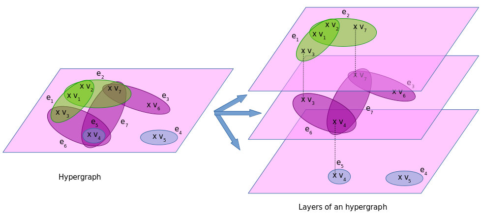
Figure 1: Illustration of a hypergraph decomposed in three layers of uniform hypergraphs

Therefore, at each $k$-uniform hypergraph $\mathcal{H}_{k}$ can be mapped a ($k$-adjacency) e-adjacency tensor $\mathcal{A}_{k}$ of order $k$ which is hypercubic and symmetric of dimension $\left|V\right|=n$. This tensor can be unnormalized or normalized.

Choosing one type of tensor - normalized or unnormalized for the whole family of $\mathcal{H}_{k}$ - the hypergraph $\mathcal{H}$ is then fully described by the family of e-adjacency tensors $\mathcal{A}_{\mathcal{H}}=\left(\mathcal{A}_{k}\right)$. In the case where all the $\mathcal{A}_{k}$ are chosen normalized this family is said pre-normalized. The final choice will be made further in Sub-Section 3.7 and explained to fullfill the expectations listed in the next Sub-Section.

3.2 Expectations for an e-adjacency tensor for a general hypergraph

The definition of the family of tensors attached to a general hypergraph has the advantage to open the way to the spectral theory for uniform hypergraphs which is quite advanced.

Nonetheless many problems remain in keeping a family of tensors of different orders: studying the spectra of the whole hypergraph could be hard to achieve by this means. Also it is necessary to get an e-adjacency tensor which covers the whole hypergraph and which retains the information on the whole structure.

The idea behind is to “fill” the hyperedges with sufficient elements such that the general hypergraph is transformed in an uniform hypergraph through a uniformisation process. A similar approach has been taken in Banerjee et al. (2017) where the filling elements are the vertices belonging to the hyperedge itself. In the next subsections the justification of the approach taken will be made via homogeneous polynomials. Before getting to the construction, expected properties of such a tensor have to be listed.

Expectation 1.

The tensor should be symmetric and its generation should be simple.

This expectation emphasizes the fact that in between two built e-adjacency tensor, the one that can be easily generated has to be chosen: it includes the fact that the tensor has to be described in a simple way.

Expectation 2.

The tensor should be invariant to vertices permutation either globally or at least locally.

This expectation is motivated by the fact that in a hyperedge the vertices have no order. The fact that this expectation can be local remains in the fact that added special vertices will not have the same status that the one from the original hypergraph. Also the invariance by permutation is expected on the vertices of the original hypergraph.

Expectation 3.

The e-adjacency tensor should allow the retrieval of the hypergraph it is originated from.

This expectation seems important to rebuild properly the original hypergraph from the e-adjacency tensor: all the necessary information to retrieve the original hyperedges has to be encoded in the tensor.

Expectation 4.

Giving the choice of two representations the sparsest e-adjacency tensor should be chosen.

Sparsity allows to compress the information and so to gain in place and complexity in calculus. Also sparsity is a desirable property for some statistical reasons as shown in Nikolova (2000) or expected in Bruckstein et al. (2009) for signal processing and image encoding.

Expectation 5.

The e-adjacency tensor should allow the retrieval of the vertex degrees.

In the adjacency matrix of a graph the information on the degrees of the vertices is encoded directly. It is still the case, as it has been seen, with the $k$-adjacency degree normalised tensor that has been defined by Shao (2013) and Pearson and Zhang (2014).

3.3 Tensors family and homogeneous polynomials family

To construct an homogeneous polynomial representing a general hypergraph, the family of e-adjacency tensors obtained in the previous Subsection is mapped to a family of homogeneous polynomials. This mapping is used in Comon et al. (2015) where the author links symmetric tensors and homogeneous polynomials of degree $s$ to show that the problem of the CP decomposition of different symmetric tensors of different orders and the decoupled representation of multivariate polynomial maps are related.

3.3.1 Homogeneous polynomials family of a hypergraph

Let $\mathbb{K}$ be a field. Here $\mathbb{K}=\mathbb{R}$.

Let $\mathcal{A}_{k}\in\mathcal{L}_{k}^{0}\left(\mathbb{K}^{n}\right)$ be a cubical tensor of order $k$ and dimension $n$ with values in $\mathbb{K}$.

Definition 15.

Let define the Segre outerproduct $\otimes$ of $\boldsymbol{a}=\left[a_{i}\right]\in\mathbb{K}^{l}$ and $\boldsymbol{b}=\left[b_{j}\right]\in\mathbb{K}^{m}$ as:

$$\boldsymbol{a}\otimes\boldsymbol{b}=\left[a_{i}b_{j}\right]_{\begin{subarray}{c}1\leqslant i\leqslant l\\ 1\leqslant j\leqslant m\end{subarray}}\in\mathbb{K}^{l\times m}.$$

More generaly as given in Comon et al. (2008) the outerproduct of $k$ vectors $u_{(1)}\in\mathbb{K}^{n_{1}}$, …, $u_{(k)}\in\mathbb{K}^{n_{k}}$ is defined as:

$$\stackrel{{\scriptstyle[}}{{i}}=1]{k}{\otimes}\boldsymbol{u_{(i)}}=\left[\prod\limits_{i=1}^{k}u_{(i)j_{i}}\right]_{j_{1},..,j_{k}=1}^{n_{1},...,n_{k}}\in\mathbb{K}^{n_{1}\times...\times n_{k}}.$$

Let $\boldsymbol{e_{1}}$, $...$, $\boldsymbol{e_{n}}$ be the canonical basis of $\mathbb{K}^{n}$.

$\left(\boldsymbol{e_{i_{1}}}\otimes...\otimes\boldsymbol{e_{i_{k}}}\right)_{1\leqslant i_{1},...,i_{k}\leqslant n}$ is a basis of $\mathcal{L}_{k}^{0}\left(\mathbb{K}^{n}\right)$.

Then $\mathcal{A}_{k}$ can be written as:

$$\mathcal{A}_{k}=\sum\limits_{1\leqslant i_{1},...,i_{k}\leqslant n}a_{(k)\,i_{1}...i_{k}}\boldsymbol{e_{i_{1}}}\otimes...\otimes\boldsymbol{e_{i_{k}}}$$

The notation $\boldsymbol{A_{k}}$ will be used for the corresponding hypermatrix of coefficients $a_{(k)\,i_{1}...i_{k}}$ where $1\leqslant i_{1},...,i_{k}\leqslant n$.

Let $z\in\mathbb{K}^{n}$, with $z=z^{i}\boldsymbol{e_{i}}$ using the Einstein convention.

In Lim (2013) a multilinear matrix multiplication is defined as follow:

Definition 16.

Let $\boldsymbol{A}\in\mathbb{K}^{n_{1}\times...\times n_{d}}$ and $X_{j}=\left[x_{(j)kl}\right]\in\mathbb{K}^{m_{j}\times n_{j}}$ for $1\leqslant j\leqslant d$.

$\boldsymbol{A^{\prime}}=\left(X_{1},...,X_{d}\right).\boldsymbol{A}$ is the multilinear matrix multiplication and defined as the matrix of $\mathbb{K}^{m_{1}\times...\times m_{d}}$ of coefficients:

$$a_{j_{1}...j_{d}}^{\prime}=\sum\limits_{k_{1},...,k_{d}=1}^{n_{1},...,n_{d}}x_{(1)j_{1}k_{1}}...x_{(d)j_{d}k_{d}}a_{k_{1}...k_{d}}$$

for $1\leqslant j_{i}\leqslant m_{i}$ with $1\leqslant i\leqslant d$.

Afterwards only vectors $z\in\mathbb{K}^{n}$ are needed and $\mathcal{A}_{k}$ is cubical of order $k$ and dimension $n$. Writing $\left(z,...,z\right)\in\left(\mathbb{K}^{n}\right)^{k}$, $\left(z\right)_{[k]}$

Therefore $(z)_{[k]}.\boldsymbol{A_{k}}$ contains only one element written $P_{k}\left(z^{1},...,z^{n}\right)=P_{k}\left(\boldsymbol{z}_{0}\right)$:

$$P_{k}\left(\boldsymbol{z}_{0}\right)=\sum\limits_{1\leqslant i_{1},...,i_{k}\leqslant n}a_{(k)\,i_{1}...i_{k}}z^{i_{1}}...z^{i_{k}}.$$ (1)

Therefore considering a hypergraph $\mathcal{H}$ with its family of unnormalized tensor $\mathcal{A}_{\mathcal{H}}=\left(\mathcal{A}_{k}\right)$, it can be also attached a family $P_{\mathcal{H}}=\left(P_{k}\right)$ of homogenous polynomials with $\deg\left(P_{k}\right)=k$.

The formulation of $P_{k}$ can be reduced taking into account that $\mathcal{A}_{k}$ is symmetric for a uniform hypergraph:

$$P_{k}\left(\boldsymbol{z}_{0}\right)=\sum\limits_{1\leqslant i_{1}\leqslant...\leqslant i_{k}\leqslant n}k!a_{(k)\,i_{1}...i_{k}}z^{i_{1}}...z^{i_{k}}.$$ (2)

Writing:

$$\widetilde{P_{k}}\left(\boldsymbol{z}_{0}\right)=\sum\limits_{1\leqslant i_{1}\leqslant...\leqslant i_{k}\leqslant n}\alpha_{(k)\,i_{1}...i_{k}}z^{i_{1}}...z^{i_{k}}.$$ (3)

the reduced form of $P_{k}$, it holds:

$$P_{k}\left(\boldsymbol{z}_{0}\right)=k!\widetilde{P_{k}}\left(\boldsymbol{z}_{0}\right).$$

Writing for $1\leqslant i_{1}\leqslant...\leqslant i_{k}\leqslant n$:

$$\alpha_{(k)\,i_{1}...i_{k}}=k!a_{(k)\,i_{1}...i_{k}}$$

and $\alpha_{(k)\,\sigma\left(i_{1}\right)...\sigma\left(i_{k}\right)}=0$ for $\sigma\in\mathcal{S}_{k}$, $\sigma\neq\text{Id}$

It holds:

$$P_{k}\left(\boldsymbol{z}_{0}\right) = \sum\limits_{1\leqslant i_{1}\leqslant...\leqslant i_{k}\leqslant n}\alpha_{(k)\,i_{1}...i_{k}}z^{i_{1}}...z^{i_{k}}$$ (4)

$$= \sum\limits_{1\leqslant i_{1},...,i_{k}\leqslant n}\alpha_{(k)\,i_{1}...i_{k}}z^{i_{1}}...z^{i_{k}}.$$

and:

$$\widetilde{P_{k}}\left(\boldsymbol{z}_{0}\right)=\sum\limits_{1\leqslant i_{1}\leqslant...\leqslant i_{k}\leqslant n}\dfrac{\alpha_{(k)\,i_{1}...i_{k}}}{k!}z^{i_{1}}...z^{i_{k}}.$$ (5)

3.3.2 Reversibility of the process

Reciprocally, given a homogeneous polynomial of degree $k$ a unique hypercubic tensor of order $k$ can be built: its dimension is the number of different variables in the homogeneous polynomial. If the homogeneous polynomial of degree $k$ is supposed reduced and ordered then only one hypercubic and symmetric hypermatrix can be built. It reflects uniquely a $k$-uniform hypergraph adding the constraint that each monomial is composed of the product of $k$ different variables.

Proposition 2.

Let $P\left(z_{0}\right)=\sum\limits_{1\leqslant i_{1},...,i_{k}\leqslant n}a_{i_{1}...i_{k}}z^{i_{1}}...z^{i_{k}}$ be a homogeneous polynomial of degree $k$ where:

• for $j\neq k$ : $z^{j}\neq z^{k}$

• for all $1\leqslant j\leqslant n$: $\deg\left(z^{j}\right)=1$

• and such that for all $\sigma\in\mathcal{S}_{k}$: $a_{\sigma\left(i_{1}\right)...\sigma\left(i_{k}\right)}=a_{i_{1}...i_{k}}$.

Then $P$ is the homogeneous polynomial attached to a unique $k$-uniform hypergraph $\mathcal{H}=\left(V,E,w\right)$ - up to the indexing of vertices.

Proof.

Considering the vertices $\left(v_{i}\right)_{1\leqslant i\leqslant n}$ labellized by the elements of $\left\llbracket 1,n\right\rrbracket$.

If $a_{i_{1}...i_{k}}\neq 0$ then for all $\sigma\in\mathcal{S}_{k}$: $a_{\sigma\left(i_{1}\right)...\sigma\left(i_{k}\right)}$ a unique hyperedge $e_{j}$ is attached corresponding to the vertices $v_{i_{1}},...,v_{i_{k}}$ and which has weight $w(e_{j})=ka_{i_{1}...i_{k}}$.

∎

3.4 Uniformisation and homogeneisation processes

A single tensor is always easier to be used than a family of tensors; the same apply for homogeneous polynomials. Building a single tensor from different order tensors requires to fill in the “gaps”; summing homogeneous polynomials of varying degrees always give a new polynomial: but, most frequently this polynomial is no more homogeneous. Homogeneisation techniques for polynomials are well known and require additional variables.

Different homogeneisation process can be envisaged to get a homogeneous polynomial that represents a single cubic and symmetric tensor by making different choices on the variables added in the homogeneisation phase of the polynomial. As a link has been made between the variables and the vertices of the hypergraph, we want that this link continue to occur during the homogeneisation of the polynomial as each term of the reduced polynomial corresponds to a unique hyperedge in the original hypergraph; the homogenisation process is interpretable in term of hypergraph uniformisation process of the original hypergraph: hypergraph uniformisation process and polynomial homogeneisation process are the two sides of the same coin.

So far, we have separated the original hypergraph $\mathcal{H}$ in layers of increasing $k$-uniform hypergraphs $\mathcal{H}_{k}$ such that

$$\mathcal{H}=\bigoplus\limits_{k=1}^{k_{\max}}\mathcal{H}_{k}.$$

Each $k$-uniform hypergraph can be represented by a symmetric and cubic tensor. This symmetric and cubic tensor is mapped to a homogeneous polynomial. The reduced homogeneous polynomial is interpretable, if we omit the coefficients of each term, as a disjunctive normal form. Each term of the homogeneous polynomial is a cunjunctive form which corresponds to simultaneous presence of vertices in a hyperedge: adding all the layers allows to retrieve the original hypergraph; adding the different homogeneous polynomials allows to retrieve the disjunctive normal form associated with the original hypergraph.

In the hypergraph uniformisation process, iterative steps are done starting with the lower layers to the upper layers of the hypergraph. In parallel, the polynomial homogeneisation process is the algebraic justification of the hypergraph uniformisation process. It allows to retrieve a polynomial attached to the uniform hypergraph built at each step and hence a tensor.

3.4.1 Hypergraph uniformisation process

We can describe algorithmically the hypergraph uniformisation process: it transforms the original hypergraph in a uniform hypergraph.

Initialisation

The initialisation requires that each layer hypergraph is associated to a weighted hypergraph.

To each uniform hypergraph $\mathcal{H}_{k}$, we associate a weighted hypergraph $\mathcal{H}_{w_{k},k}=\left(V,E_{k},w_{k}\right)$, with: $\forall e\in E_{k}:w_{k}(e)=c_{k}$, $c_{k}\in\mathbb{R}^{+*}$.

The coefficients $c_{k}$ are technical coefficients that will be chosen when considering the homogeneisation process and the fullfillment of the expectations of the e-adjacency tensor. The coefficients $c_{k}$ can be seen as dilatation coefficients only dependent of the layers of the original hypergraph.

We initialise:

$k:=1$ and $\mathcal{K}_{w}:=\mathcal{H}_{w_{1},1}$

and generate $k_{\max}-1$ distinct vertices $y_{j}$, $j\in\left\llbracket 1,k_{\max}-1\right\rrbracket$ that are not in $V$.

Iterative steps

Each step in the hypergraph uniformisation process includes three phases: an inflation phase, a merging phase and a concluding phase.

Inflation phase:

The inflation phase consists in increasing the cardinality of each hyperedge obtained from the hypergraph built at the former step to reach the cardinality of the hyperedges of the second hypergraph used in the merge phase.

Definition 17.

The $y$-vertex-augmented hypergraph of a weighted hypergraph $\mathcal{H}_{w}=\left(V,E,w\right)$ is the hypergraph $\overline{\mathcal{H}_{\overline{w}}}=\left(\overline{V},\overline{E},\overline{w}\right)$ obtained by the following rules

• $y\notin V$;

• $\overline{V}=V\cup\left\{y\right\}$;

• Writing $\phi:\mathcal{P}\left(V\right)\rightarrow\mathcal{P}\left(\overline{V}\right)$ the map such that for $A\in\mathcal{P}\left(V\right):\,$$\phi(A)=A\cup\left\{y\right\}$, it holds:

  • $\overline{E}=\left\{\phi\left(e\right):e\in E\right\}$;

  • $\forall e\in E$, $\overline{w}\left(\phi(e)\right)=w(e)$.

Proposition 3.

The vertex-augmented hypergraph of a $k$-uniform hypergraph is a $k+1$-uniform hypergraph.

The inflation phase at step $k$ generates from $\mathcal{K}_{w}$ the $y_{k}$-vertex augmented hypergraph $\overline{\mathcal{K}_{\overline{w}}}$.

As $\mathcal{K}_{w}$ is $k$-uniform at step $k$, $\overline{\mathcal{K}_{\overline{w}}}$ is $k+1$-uniform

Merging phase:

The merging phase generates the sum of two weighted hypergraphs called the merged hypergraph.

Definition 18.

The merged hypergraph $\widehat{\mathcal{H}_{\widehat{w}}}=\left(\widehat{V},\widehat{E},\widehat{w}\right)$ of two weighted hypergraphs $\mathcal{H}_{a}=\left(V_{a},E_{a},w_{a}\right)$ and $\mathcal{H}_{b}=\left(V_{b},E_{b},w_{b}\right)$ is the weighted hypergraph defined as follow:

• $\widehat{V}=V_{a}\cup V_{b}$

• $\widehat{E_{k+1}}=E_{a}\cup E_{b}$

• $\forall e\in E_{a}:\,\widehat{w}(e)=\overline{w_{a}}(e)$ and $\forall e\in E_{b}:\,\widehat{w}(e)=w_{b}$

The merging phase at step $k$ generates from $\overline{\mathcal{K}_{w}}$ and $\mathcal{H}_{d,k+1}$ the merged hypergraph $\widehat{\mathcal{K}_{\widehat{w}}}$. As it is generated from two $k+1$-uniform hypergraph it is also a $k+1$-uniform hypergraph.

Step ending phase:

If $k$ equals $k_{\text{max}}-1$ the iterative part ends up and return $\widehat{\mathcal{K}_{\widehat{w}}}$.

Otherwise a next step is need with $\mathcal{K}_{w}:=\widehat{\mathcal{K}_{\widehat{w}}}$ and $k:=k+1$.

Termination:

We obtain by this algorithm a weighted $k_{\max}$-uniform hypergraph associated to $\mathcal{H}$ which is the returned hypergraph from the iterative part: we write it $\widehat{\mathcal{H}_{\widehat{w}}}=\left(\widehat{V},\widehat{E},\widehat{w}\right)$.

Definition 19.

Writing $V_{s}=\left\{y_{j}:j\in\left\llbracket 1,k_{\max}-1\right\rrbracket\right\}$

$\widehat{\mathcal{H}_{\widehat{w}}}=\left(\widehat{V},\widehat{E},\widehat{w}\right)$ is called the $V_{s}$-layered unifom of $\mathcal{H}$.

Proposition 4.

Let $\mathcal{H}=\left(V,E\right)$ be a hypergraph of order $k_{\max}$

Let consider $V_{s}=\left\{y_{j}:j\in\left\llbracket 1,k_{\max}-1\right\rrbracket\right\}$ such that $V\cap V_{s}=\emptyset$ and let $\widehat{\mathcal{H}_{\widehat{w}}}=\left(\widehat{V},\widehat{E},\widehat{w}\right)$ be the $V_{s}$-layered unifom of $\mathcal{H}$. Then:

• $\left(V,V_{s}\right)$ is a partition of $\widehat{V}$.

• $\forall e\in E,\exists!\widehat{e}\in\widehat{E}:e\subseteq\widehat{e}\land\widehat{e}\backslash e=\left\{y_{j}:j\in\left\llbracket\left|e\right|,k_{\max}-1\right\rrbracket\right\}.$

Proof.

The way the $V_{s}$-layered uniform of $\mathcal{H}$ is generated justifies the results.

∎

Proposition 5.

Let $\mathcal{H}=\left(V,E\right)$ be a hypergraph of order $k_{\max}$

Let consider $V_{s,i}=\left\{y_{j}:j\in\left\llbracket i,k_{\max}-1\right\rrbracket\right\}$ such that $V_{s}=\bigcup\limits_{i\in\left\llbracket 1,k_{\max}-1\right\rrbracket}V_{s,i}$, $V\cap V_{s}=\emptyset$ and let $\widehat{\mathcal{H}_{\widehat{w}}}=\left(\widehat{V},\widehat{E},\widehat{w}\right)$ be the $V_{s}$-layered unifom of $\mathcal{H}$.

Then:

Vertices of $\mathcal{H}$ that are e-adjacent in $\mathcal{H}$ in an hyperedge $e$ are e-adjacent with the vertices of $V_{s,\left|e\right|}$ in $\widehat{\mathcal{H}_{\widehat{w}}}$.

Reciprocally, if vertices are e-adjacent in $\widehat{\mathcal{H}_{\widehat{w}}}$, the ones that are not in $V_{s}$ are e-adjacent in $\mathcal{H}$.

As a consequence, $\widehat{\mathcal{H}_{\widehat{w}}}$ captures the e-adjacency of $\mathcal{H}$.

3.4.2 Polynomial homogeneisation process

In the polynomial homogeneisation process, we build a new family $R_{\mathcal{H}}=\left(R_{k}\right)$ of homogeneous polynomials of degree $k$ iteratively from the family of homogeneous polynomials $P_{\mathcal{H}}=\left(P_{k}\right)$ by following the subsequent steps that respect the phases of construction in Figure 2. Each of these steps can be linked to the steps of the homogeneisation process.

Figure 2: Different phases of the construction of the e-adjacency tensor

Initialisation

Each polynomial $P_{k}$, $k\in\left\llbracket 1,k_{\max}\right\rrbracket$ attached to the corresponding layer $k$-uniform hypergraph $\mathcal{H}_{k}$ is multiplied by a coefficient $c_{k}$ equals to the dilatation coefficients of the hypergraph uniformisation process. $c_{k}P_{k}$ represents the reduced homogeneous polynomial attached to $\mathcal{H}_{w_{k},k}$.

We initialise:

$k:=1$ and $R_{k}\left(\boldsymbol{z}_{k-1}\right)=R_{1}\left(\boldsymbol{z}_{o}\right)=c_{1}P_{1}\left(\boldsymbol{z}_{o}\right)=c_{1}\sum\limits_{i=1}^{n}a_{(1)\,i}z^{i}.$

We generate $k_{\max}-1$ distinct 2 by 2 variables $y^{j}$, $j\in\left\llbracket 1,k_{\max}-1\right\rrbracket$ that are also distinct 2 by 2 from the $z^{i}$, $i\in\left\llbracket 1,n\right\rrbracket$.

Iterative steps

At each step, we sum the current $R_{k}\left(z_{k-1}\right)$ with the next layer coefficiented polynomial $c_{k+1}P_{k+1}$ in a way to obtain a homogeneous polynomial $R_{k+1}\left(z_{k}\right)$. To help the understanding we describe the first step, then generalise to any step.

Case $k=1$: To build $R_{2}$ an homogeneization of the sum of $R_{1}$ and $c_{2}P_{2}$ is needed. It holds:

$$R_{1}\left(\boldsymbol{z}_{o}\right)+c_{2}P_{2}\left(\boldsymbol{z}_{o}\right)=c_{1}\sum\limits_{i=1}^{n}a_{(1)\,i}z^{i}+c_{2}\sum\limits_{i_{1},i_{2}=1}^{n}a_{(2)\,i_{1}i_{2}}z^{i_{1}}z^{i_{2}}$$

To achieve the homogeneization of $R_{1}\left(\boldsymbol{z}_{o}\right)+c_{2}P_{2}\left(\boldsymbol{z}_{o}\right)$ a new variable $y^{1}$ is introduced.

It follows for $y^{1}\neq 0$:

$$R_{2}\left(\boldsymbol{z}_{1}\right) = R_{2}\left(z_{0},y^{1}\right)$$

$$= y^{1(2)}\left(R_{1}\left(\dfrac{z_{0}}{y^{1}}\right)+c_{2}P_{2}\left(\dfrac{z_{0}}{y^{1\,(2)}}\right)\right)$$

$$= c_{1}\sum\limits_{i=1}^{n}a_{(1)\,i}z^{i}y^{1}+c_{2}\sum\limits_{i_{1},i_{2}=1}^{n}a_{(2)\,i_{1}i_{2}}z^{i_{1}}z^{i_{2}}.$$

By continuous prolongation of $R_{2}$, it is set:

$$R_{2}\left(\boldsymbol{z}_{o},0\right)=c_{2}\sum\limits_{i_{1},i_{2}=1}^{n}a_{(2)\,i_{1}i_{2}}z^{i_{1}}z^{i_{2}}.$$

In this step, the degree 1 coefficiented polynomial $R_{1}\left(z_{0}\right)=c_{1}P_{1}\left(z_{0}\right)$ attached to $\mathcal{H}_{w_{1},1}$ is transformed in a degree 2 homogeneous polynomial $y^{1}R_{1}\left(z_{0}\right)=c_{1}y^{1}P_{1}\left(z_{0}\right)$: $y^{1}R_{1}\left(z_{0}\right)$ corresponds to the homogeneous polynomial of the weighted $y_{1}$-vertex-augmented 1-uniform hypergraph $\overline{\mathcal{H}_{\overline{w_{1}},1}}$ built during the inflation phase in the hypergraph uniformisation process.

$y_{1}R_{1}\left(z_{0}\right)$ is then summed with the homogeneous polynomial $c_{2}P_{2}$ attached to $\mathcal{H}_{w_{2},2}$ to get an homogeneous polynomial of degree 2: $R_{2}\left(z_{1}\right)$. $R_{2}\left(z_{1}\right)$ is the homogeneous polynomial of the merged 2-uniform hypergraph $\widehat{\mathcal{H}_{\widehat{w_{1}},1}}$ of $\overline{\mathcal{H}_{w_{1},1}}$ and $\mathcal{H}_{w_{2},2}$.

General case: Supposing that $R_{k}\left(\boldsymbol{z}_{k-1}\right)$ is an homogeneous polynomial of degree $k$ that can be written as:

$$R_{k}\left(\boldsymbol{z}_{k-1}\right)=\sum\limits_{j=1}^{k}c_{j}\sum\limits_{i_{1},...,i_{j}=1}^{n}a_{(j)\,i_{1}...i_{j}}z^{i_{1}}...z^{i_{j}}\prod\limits_{l=j}^{k-1}y^{l},$$

with the convention that: $\prod\limits_{l=j}^{k-1}y^{l}=1$ if $j>k-1$ and $\omega_{k-1}=z^{1},...,z^{n},y^{1},...,y^{k-1}$

$R_{k+1}$ is built as an homogeneous polynomial from the sum of $R_{k}$ and $c_{k+1}P_{k+1}$ by adding a variable $y_{k}$ and factorizing by its $k+1$-th power.

Therefore, for $y^{k-1}\neq 0$:

$$R_{k+1}\left(\boldsymbol{z}_{k}\right) = y^{k\,(k+1)}\left(R_{k}\left(\dfrac{\boldsymbol{z}_{k-1}}{y^{k\,(k)}}\right)+c_{k+1}P_{k+1}\left(\dfrac{\boldsymbol{z}_{o}}{y^{k\,(k+1)}}\right)\right)$$

$$= \left(\sum\limits_{j=1}^{k}c_{j}\sum\limits_{i_{1},...,i_{j}=1}^{n}a_{(j)\,i_{1}...i_{j}}z^{i_{1}}...z^{i_{j}}\prod\limits_{l=j}^{k-1}y^{l}\right)y^{k}$$

$$+c_{k+1}\sum\limits_{i_{1},...,i_{k+1}=1}^{n}a_{(k+1)\,i_{1}\,...\,i_{k+1}}z^{i_{1}}...z^{i_{k+1}}$$

And for $y_{k}=0$, it is set by continuous prolongation: $R_{k+1}\left(\boldsymbol{z}_{k-1},0\right)=c_{k+1}\sum\limits_{i_{1},...,i_{k+1}=1}^{n}a_{(k+1)\,i_{1}\,...\,i_{k+1}}z^{i_{1}}...z^{i_{k+1}}.$

The fact that $P_{k+1}\left(z_{0}\right)$ can be null doesn’t prevent to do the step: the degree of $R_{k}$ will then be elevated of 1.

The interpretation of this step is similar to the one done for the case $k=1$.

Step ending phase:

If $k$ equals $k_{\text{max}}-1$ the iterative part ends up, else $k:=k+1$ and the next iteration is started.

Conclusion

The algorithm build a family of homogeneous polynomial which is interpretable in term of uniformisation of a hypergraph.

3.5 Building an unnormalized symmetric tensor from this family of homogeneous polynomials

Based on $R_{\mathcal{H}}$

It is now valuable to interpret the built polynomials.

The notation $\boldsymbol{w}_{(k)}=w_{(k)}^{1},...,w_{(k)}^{n+k-1}$ is used.

• The interpretation of $R_{1}$ is trivial as it holds the single element hyperedges of the hypergraph.

• $R_{2}$ is an homogeneous polynomial with $n+1$ variables of order 2.

  $$R_{2}\left(\boldsymbol{z}_{1}\right) = c_{1}\sum\limits_{i=1}^{n}a_{(1)\,i}z^{i}y^{1}+c_{2}\sum\limits_{i_{1},i_{2}=1}^{n}a_{(2)\,i_{1}i_{2}}z^{i_{1}}z^{i_{2}}$$

  $$= c_{1}\sum\limits_{1\leqslant i\leqslant n}\alpha_{(1)\,i}z^{i}y^{1}+c_{2}\sum\limits_{1\leqslant i_{1}\leqslant i_{2}\leqslant n}\alpha_{(2)\,i_{1}i_{2}}z^{i_{1}}z^{i_{2}}$$

  It can be rewritten:

  $$R_{2}\left(\boldsymbol{w}_{(2)}\right)=\sum\limits_{i_{1},i_{2}=1}^{n+1}r_{(2)\,i_{1}i_{2}}w_{(2)}^{i_{1}}w_{(2)}^{i_{2}}$$

  where:

  • for $1\leqslant i\leqslant n$: $w_{(2)}^{i}=z^{i}$

  • $w_{(2)}^{n+1}=y^{1}$

  • for $1\leqslant i_{1}\leqslant i_{2}\leqslant n$ and $\sigma\in\mathcal{S}_{2}$:

    $$r_{(2)\,\sigma\left(i_{1}\right)\sigma\left(i_{2}\right)}=\dfrac{c_{2}\alpha_{(2)\,i_{1}i_{2}}}{2!}=c_{2}a_{(2)\,i_{1}i_{2}}$$

  • for $1\leqslant i\leqslant n$ and $\sigma\in\mathcal{S}_{2}$:

    $$r_{(2)\,\sigma(i)\,\sigma(n+1)}=\dfrac{c_{1}\alpha_{(1)\,i}}{2!}=\dfrac{c_{1}a_{(1)\,i}}{2!}$$

  • the other coefficients: $r_{(2)\,i_{1}i_{2}}$ are null.

  Also $R_{2}$ can be linked to a symmetric hypercubic tensor of order 2 and dimension $n+1$.

• $R_{k}$ is an homogeneous polynomial with $n+k-1$ variables of order $k$.

  $$R_{k}\left(\boldsymbol{z}_{k-1}\right) = \sum\limits_{j=1}^{k}c_{j}\sum\limits_{i_{1},...,i_{j}=1}^{n}a_{(j)\,i_{1}...i_{j}}z^{i_{1}}...z^{i_{j}}\prod\limits_{l=j}^{k-1}y^{l}$$

  $$= \sum\limits_{j=1}^{k}c_{j}\sum\limits_{1\leqslant i_{1}\leqslant...\leqslant i_{j}\leqslant n}\alpha_{(j)\,i_{1}...i_{j}}z^{i_{1}}...z^{i_{j}}\prod\limits_{l=j}^{k-1}y^{l}$$

  with the convention that: $\prod\limits_{l=j}^{k-1}y^{l}=1$ if $j>k-1$.

  It can be rewritten:

  $$R_{k}\left(\boldsymbol{w}_{(k)}\right)=\sum\limits_{i_{1},...,i_{k}=1}^{n+k-1}r_{(k)\,i_{1}\,...\,i_{k}}w_{(k)}^{i_{1}}...w_{(k)}^{i_{k}}$$

  where:

  • for $1\leqslant i\leqslant n$: $w_{(k)}^{i}=z^{i}$

  • for $n+1\leqslant i\leqslant n+k-1$: $w_{(k)}^{i}=y^{i-n}$

  • for $1\leqslant i_{1}\leqslant...\leqslant i_{k}\leqslant n$, for all $1\leqslant j\leqslant k-1$, for all $\sigma\in\mathcal{S}_{k}$:

    • $r_{(k)\,\sigma\left(i_{1}\right)...\sigma\left(i_{k}\right)}=\dfrac{c_{k}\alpha_{(k)\,i_{1}...i_{k}}}{k!}=c_{k}a_{(k)\,i_{1}...i_{k}}$

    • $r_{(k)\,\sigma\left(i_{1}\right)...\sigma\left(i_{j}\right)\sigma(n+j)...\sigma(n+k-1)}=\dfrac{c_{j}\alpha_{(j)\,i_{1}...i_{j}}}{k!}=\dfrac{j!}{k!}c_{j}a_{(j)\,i_{1}...i_{j}}$

  • the other elements $r_{(k)\,i_{1}\,...\,i_{k}}$ are null.

  Also $R_{k}$ can be linked to a symmetric hypercubic tensor of order $k$ and dimension $n+k-1$ written $\boldsymbol{R_{k}}$ whose elements are $r_{(k)\,i_{1}\,...\,i_{k}}$.

The hypermatrix $\boldsymbol{R_{k_{\max}}}$ is called the unnormalized tensor.

3.6 Interpretation and choice of the coefficients for the unnormalized tensor

There are different ways of setting the coefficients $c_{1},...,c_{k_{\text{\text{max}}}}$ that are used. These coefficients can be seen as a way of normalizing the tensors of e-adjacency generated from the $k$-uniform hypergraphs.

A first way of choosing them is to set them all equal to 1. In this case no normalization occurs. The impact on the e-adjacency tensor of the original hypergraph is that e-adjacency in hyperedges of size $k$ have a weight of $k$ times bigger than the e-adjacency in hyperedges of size 1.

A second way of choosing these coefficients is to consider that in a $k$-uniform hypergraph, each hyperedge holds $k$ vertices and then contributes to $k$ to the total degree. Representing this $k$-uniform hypergraph by the $k-$adjacency degree normalized tensor $\mathcal{A}_{k}=\left(a_{(k)\,i_{1}...i_{k}}\right)_{1\leqslant i_{1},...,i_{k}\leqslant n}$, it holds a revisited hand-shake lemma for $k$-uniform hypergraphs:

$$\sum\limits_{1\leqslant i_{1},...,i_{k}\leqslant n}a_{(k)\,i_{1}...i_{k}} = \sum\limits_{i=1}^{n}\sum\limits_{1\leqslant i_{2},...,i_{k}\leqslant n}a_{(k)\,ii_{2}...i_{k}}$$

$$= \sum\limits_{i=1}^{n}d_{(k)\,i}$$

$$= k\left|E_{k}\right|$$

where $d_{(k)\,i}$ is the degree of the vertex $v_{i}$ in $\mathcal{H}_{k}$.

This formula can be extended to general hypergraphs:

$$\left|E\right| = \sum\limits_{k=1}^{k_{\text{\text{max}}}}\left|E_{k}\right|$$

$$= \sum\limits_{k=1}^{k_{\text{\text{max}}}}\dfrac{1}{k}\sum\limits_{i=1}^{n}d_{(k)\,i}$$

$$= \sum\limits_{k=1}^{k_{\text{\text{max}}}}\dfrac{1}{k}\sum\limits_{1\leqslant i_{1},...,i_{k}\leqslant n}a_{(k)\,i_{1}...i_{k}}.$$

For general hypergraphs, the tensor is of order $k_{\max}$.

$$\sum\limits_{1\leqslant i_{1},...,i_{k_{\max}}\leqslant n+k_{\max}-1}r_{i_{1}...i_{k_{\max}}} = \sum\limits_{i=1}^{n+k_{\max}-1}\sum\limits_{1\leqslant i_{2},...,i_{k}\leqslant n+k_{\max}-1}r_{ii_{2}...i_{k_{\max}}}$$

$$= \sum\limits_{i=1}^{n}\deg\left(v_{i}\right)+\sum\limits_{i=n+1}^{n+k_{\max}-1}\deg\left(y_{i}\right)$$

The constructed tensor corresponds to the tensor of a $k_{\max}$-uniform hypergraph with $n+k_{\max}-1$ vertices. It holds:

$$\sum\limits_{1\leqslant i_{1},...,i_{k_{\max}}\leqslant n+k_{\max}-1}r_{i_{1}...i_{k_{\max}}}=k_{\max}\text{$\left|E\right|$}.$$

And therefore:

$$\sum\limits_{1\leqslant i_{1},...,i_{k_{\max}}\leqslant n+k_{\max}-1}r_{i_{1}...i_{k_{\max}}}=\sum\limits_{k=1}^{k_{\text{\text{max}}}}\dfrac{k_{\max}}{k}\sum\limits_{1\leqslant i_{1},...,i_{k}\leqslant n}a_{(k)\,i_{1}...i_{k}}.$$

Also $c_{k}=\dfrac{k_{\max}}{k}$ seems to be a good choice in this case.

The final choice will be taken in the next paragraph to answer to the required specifications on degrees. It will also fix the matrix chosen for the uniform hypergraphs.

3.7 Unnormalized e-adjacency tensor’s expectations fulfillment

Guarantee 1.

The tensor should be symmetric and its generation should be simple.

Proof.

By construction the e-adjacency tensor is symmetric. To generate it only one element has to be described for a given hyperedge the other elements obtained by permutation of the indices being the same. Also the built e-adjacency tensor is fully described by giving $\left|E\right|$ elements.

∎

Guarantee 2.

The unnormalized e-adjacency tensor keeps the overall structure of the hypergraph.

Proof.

It is inherent to the way the tensor has been built: the layer of level equal or under $j$ can be seen in the mode 1 at the $n+j$-th component of the mode. To have only elements of level $j$ one can project this mode so that it keeps only the first $n$ dimensions.∎

In the expectations of the built co-tensors listed in the paragraph 3.2, the e-adjacency tensor should allow the retrieval of the degree of the vertices. It implies to fix the choice of the $k$-adjacency tensors used to model each layer of the hypergraph as well as the normalizing coefficient.

Let consider for $1\leqslant k\leqslant k_{\max}$, $2\leqslant l\leqslant k_{\max}$ and $1\leqslant i\leqslant n+k_{\max}-1$:

$$I_{k,l,i}=\left\{\left(i_{1},...,i_{l}\right):i_{1}=i\land\forall j\in\left\llbracket 2,l\right\rrbracket:1\leqslant i_{j}\leqslant n+k-1\right\}$$

and its subset of ordered tuples

$$OI_{k,l,i}=\left\{\left(i_{1},...,i_{l}\right):\left(i_{1},...,i_{l}\right)\in I_{k,l,i}\land\left(l\geqslant 2\implies\forall\left(j_{1},j_{2}\right)\in\left\llbracket 2,l\right\rrbracket^{2}:j_{1}<j_{2}\implies i_{j_{1}}<i_{j_{2}}\right)\right\}.$$

Then:

$$\sum\limits_{\left(i_{1},...,i_{k_{\text{\text{max}}}}\right)\in I_{k_{\text{\text{max}}},k_{\text{\text{max}}},i}}r_{i_{1}...i_{k_{\text{max}}}} = \sum\limits_{\left(i_{1},...,i_{k_{\text{\text{max}}}}\right)\in OI_{k_{\text{\text{max}}},k_{\text{\text{max}}},i}}\left(k_{\text{\text{max}}}-1\right)!r_{i_{1}...i_{k_{\text{\text{max}}}}}$$

$$= \sum\limits_{j=1}^{k_{\text{\text{max}}}}\sum\limits_{\left(i_{1},...,i_{j}\right)\in OI_{k_{\text{\text{max}}},j,i}}\dfrac{j!c_{j}a_{(j)\,i_{1}...i_{j}}}{k_{\max}}$$

Hence, the expectation on the retrieval of degree imposes to set $c_{j}a_{(j)\,i_{1}...i_{j}}=\dfrac{k_{\max}}{j!}$ for the elements of $\mathcal{A}_{(j)}$ that are not null, which is coherent with the usage of the coefficient $c_{j}=\dfrac{k_{\max}}{j}$ and of the degree-normalized tensor for $j$-uniform hypergraph where not null elements are equals to: $\dfrac{1}{(j-1)!}$. This choice is then made for the rest of the article.

Remark 1.

By choosing $c_{j}=\dfrac{k_{\max}}{j}$ and the degree-normalized tensor for $j$-uniform hypergraph where not null elements are equals to: $\dfrac{1}{(j-1)!}$, it follows that: $r_{i_{1}...i_{k_{\text{\text{max}}}}}=\dfrac{1}{\left(k_{\text{\text{max}}}-1\right)!}$ for all elements which is consistent with the fact that we have built a $k_{\max}$-uniform hypergraph by filling each hyperedge with additional vertices. This method is similar to make a plaster molding from a footprint in the sand: the filling elements help reveal the structure behind.

With this choice, writing $\mathds{1}_{e\in E}:\begin{cases}1&\text{if }e\in E\\ 0&\text{otherwise}\end{cases}.$

$$\sum\limits_{\left(i_{1},...,i_{k_{\text{\text{max}}}}\right)\in I_{k_{\text{\text{max}}},k_{\text{\text{max}}},i}}r_{i_{1}...i_{k_{\text{\text{max}}}}} = \sum\limits_{j=1}^{k_{\text{\text{max}}}}\sum\limits_{\left(i_{1},...,i_{j}\right)\in OI_{k_{\text{\text{max}}},j,i}}\mathds{1}_{\left\{v_{i_{1}},...,v_{i_{j}}\right\}\in E}.$$

It follows immediately:

Guarantee 3.

The unnormalized e-adjacency tensor allows the retrieval of the degree of the vertices of the hypergraph.

Proof.

Defining for $1\leqslant i\leqslant n$: $d_{i}=\deg\left(v_{i}\right)$.

From the previous choice, it follows that:

$$\sum\limits_{\left(i_{1},...,i_{k_{\text{\text{max}}}}\right)\in I_{k_{\text{\text{max}}},k_{\text{\text{max}}},i}}r_{i_{1}...i_{k_{\text{\text{max}}}}} = \sum\limits_{\left(i_{1},...,i_{k_{\text{\text{max}}}}\right)\in OI_{k_{\text{\text{max}}},k_{\text{\text{max}}},i}}\left(k_{\text{\text{max}}}-1\right)!r_{i_{1}...i_{k_{\text{\text{max}}}}}$$

$$= \sum\limits_{j=1}^{k_{\text{\text{max}}}}\sum\limits_{\left(i_{1},...,i_{j}\right)\in OI_{k_{\text{\text{max}}},j,i}}\dfrac{j!c_{j}a_{(j)\,i_{1}...i_{j}}}{k_{\max}}$$

$$= \sum\limits_{j=1}^{k_{\text{\text{max}}}}\sum\limits_{\left(i_{1},...,i_{j}\right)\in OI_{k_{\text{\text{max}}},j,i}}\mathds{1}_{\left\{v_{i_{1}},...,v_{i_{j}}\right\}\in E}$$

$$= \deg\left(v_{i}\right)$$

as $\dfrac{j!c_{j}a_{(j)\,i_{1}...i_{j}}}{k_{\max}}=1$ only for hyperedges where $v_{i}$ is in it (and they are counted only once for each hyperedge).

∎

Guarantee 4.

The unnormalized e-adjacency tensor allows the retrieval of the cardinality of the hyperedges.

Proof.

Defining $d_{n+i}=\left|\left\{e\,:\,\left|e\right|\leqslant i\right\}\right|$ for $1\leqslant i\leqslant k_{\max}$.

$$\sum\limits_{\left(i_{1},...,i_{k_{\text{\text{max}}}}\right)\in I_{k_{\text{max}},k_{\text{\text{max}}},n+i}}r_{i_{1}...i_{k_{\text{max}}}} = \sum\limits_{j=1}^{i}\sum\limits_{1\leqslant l_{1}<...<l_{j}\leqslant n}\left(k_{\text{\text{max}}}-1\right)!\dfrac{j!c_{j}a_{(j)\,i_{1}...i_{j}}}{k_{\max}!}$$

$$= \sum\limits_{j=1}^{i}\sum\limits_{1\leqslant l_{1}<...<l_{j}\leqslant n}\mathds{1}_{\left\{v_{l_{1}},...,v_{l_{j}}\right\}\in E}$$

due to the fact that $r_{n+i\,i_{2}...i_{k_{\text{max}}}}\neq 0$ if and only if it exists at most $i$ indices $i_{2}$ to $i_{k_{\max}}$ that are between 1 and $n$ which correspond to vertices in the general hypergraph and the other indices have value strictly above $n$ which represent additional vertices.

It follows:

$$\sum\limits_{\left(i_{1},...,i_{k_{\text{\text{max}}}}\right)\in I_{k_{\text{\text{max}}},k_{\text{\text{max}}},n+i}}r_{i_{1}...i_{k_{\text{\text{max}}}}} = d_{n+i}.$$

We set: $d_{n+k_{\max}}=\left|E\right|$.

Also $d_{n+j}$ allows to retrieve the number of hyperedges of cardinality equal or less than $j$.

Therefore:

• for $2\leqslant j\leqslant k_{\max}$: $\left|\left\{e\,:\,\left|e\right|=j\right\}\right|=d_{n+j}-d_{n+j-1}$

• for $j=1$: $\left|\left\{e\,:\,\left|e\right|=1\right\}\right|=d_{n+1}$

An other way of keeping directly the cardinality of the layer $k_{\max}$ in the e-adjacency tensor would be to store it in an additional variable $y_{k_{\max}}$.

∎

Guarantee 5.

The e-adjacency tensor is unique up to the labeling of the vertices for a given hypergraph.

Reciprocally, given the e-adjacency tensor and the number of vertices, the associated hypergraph is unique.

Proof.

Given a hypergraph, the process of decomposition in layers is bijective as well as the formalization by degree normalized $k$-adjacency tensor. Given the coefficients, the process of building the e-adjacency homogeneous polynomial is also unique and the reversion to a symmetric cubic tensor is unique.

Given the e-adjacency tensor and the number of vertices, as the e-adjacency tensor is symmetric, up to the labeling of the vertices, considering that the first $n$ variables encoded in the e-adjacency tensor in each direction represents variables associated to vertices of the hypergraph and the last variables in each direction encode the information of cardinality. Therefore it is possible to retrieve each layer of the hypergraph uniquely and consequently the whole hypergraph.

∎

3.8 Interpretation of the e-adjacency tensor

The general hypergraph layer decomposition allows to retrieve uniform hypergraphs that can be separately modeled by e-adjacency (or equivalently $k$-adjacency) tensor of $k$-uniform hypergraphs. We have shown that filling these different layers with additional vertices allow to uniformize the original hypergraph by keeping the e-adjacency. The coefficients used in the iterative process has to be seen as weights on the hyperedges of the final $k_{\max}$-uniform hypergraph: these coefficients allow to retrieve the right number of edges from the uniformized hypergraph tensor so that it corresponds to the number of edges of the original hypergraph.

The additional dimensions in the e-adjacency tensor allows to retrieve the cardinality of the hyperedges. By decomposing a hypergraph in a set of uniform hypergraphs the hyperedges are quotiented depending on their cardinality.

The iterative approach principle is illustrated in Figure3: vertices that are added at each level give indication on the original cardinality of the hyperedge it is added to.

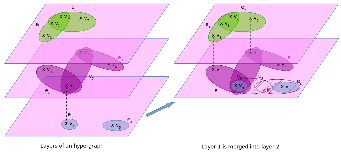
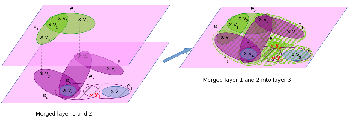
Figure 3: Illustration of the iterative approach concept on an example

In the iterative approach the layers of level $n$ and $n+1$ are merged together into the layer $n+1$ by adding a filling vertex to the hyperedges of the layer $n$. On this example, during the first step the layer 1 and 2 are merged to form a 2-uniform hypergraph. In the second step, the 2-uniform hypergraph obtained in the first step is merged to the layer 3 to obtain a 3-uniform hypergraph.

Viewed in an other way, e-adjacency hypermatrix of uniform hypergraph don’t need an extra dimension as the hyperedges are uniform, therefore there is no ambiguity. Adding an extra variable allows to capture the dimensionality of each hyperedge meanwhile preventing any ambiguity on the meaning of each element of the tensor.

4 Some comments on the e-adjacency tensor

4.1 The particular case of graphs

As a graph $G=\left(V,E\right)$ with $\left|V\right|=n$ can always be seen a $2$-uniform hypergraph $\mathcal{H}_{G}$, the approach given in this paragraph should allow to retrieve in a coherent way the spectral theory for normal graphs.

The hypergraph that contains the 2-uniform hypergraph is then composed of an empty level 1 layer and a level 2 layer that contains only $\mathcal{H}_{G}$.

Let $A$ be the adjacency matrix of $G$. The e-adjacency tensor of the corresponding 2-uniform hypergraph is of order 2 and obtained from $A$ by multiplying it by $c_{2}$ and adding one row and one column of zero. Therefore the e-adjacency tensor of the two level of the corresponding hypergraph is: $\mathcal{A}$= $\left(\begin{array}[]{c|c}c_{2}A&0\\ \hline\cr 0&0\end{array}\right)$

Also as an eigenvalue $\lambda$ of $\mathcal{A}$ seen as a matrix is a solution of the characteristic polynomial $\det\left(\mathcal{A}-\lambda I\right)=0\Leftrightarrow-\lambda\det\left(c_{2}A-\lambda I\right)=0\Leftrightarrow-\lambda c_{2}^{n}\det\left(A-\dfrac{\lambda}{c_{2}}I\right)=0$, the eigenvalues of $\mathcal{A}$ are $c_{2}$times the ones of $A$ and one additional 0 eigenvalue. This last eigenvalue is attached to the eigenvector $\left(0...0\,1\right)^{T}$. The other eigenvalues have same eigenvectors than $A$ with one additional $n+1$ component which is 0.

Proof.

Let consider $Y=\left(\begin{array}[]{c}X\\ y\end{array}\right)$ with $X$ vector of dimension n. Let $\lambda$ be an eigenvalue of $\mathcal{A}$ and $Y$ an eigenvector of $\mathcal{A}$

$\mathcal{A}Y=\lambda Y\Leftrightarrow\mathcal{A}\left(\begin{array}[]{c}X\\ y\end{array}\right)=\lambda\left(\begin{array}[]{c}X\\ y\end{array}\right)\Leftrightarrow\left(c_{2}A-\lambda I_{n}\right)X=0\land-\lambda y=0\Leftrightarrow X$ eigenvalue of $A$ attached to $\dfrac{\lambda}{c_{2}}$. $y$ can be always taken equals to 0 to fit the second condition.

∎

Therefore globally there is no change in the spectra: the eigenvectors hold, the eigenvalues of the initial graph are multiplied by the normalizing coefficient.

4.2 e-adjacency tensor and DNF

Let $\mathcal{H}=\left(V,E\right)$ be a hypergraph, $\mathcal{A}$ its e-adjacency tensor and $\tilde{R}_{k_{\max}}$ the reduced attached homogeneous polynomial.

$$\tilde{R}_{k_{\max}}\left(\boldsymbol{w}_{\left(k_{\max}\right)}\right)=\sum\limits_{1\leqslant i_{1}<...<i_{k}\leqslant n+k_{\max}-1}\tilde{r}_{\left(k_{\max}\right)\,i_{1}\,...\,i_{k_{\max}}}w_{(k_{\max})}^{i_{1}}...w_{(k_{\max})}^{i_{k_{\max}}}$$

with $\tilde{r}_{\left(k_{\max}\right)\,i_{1}\,...\,i_{k_{\max}}}=k_{\max}!r_{\left(k_{\max}\right)\,i_{1}\,...\,i_{k_{\max}}}$

The variables $\left(w_{(k_{\max})}^{i}\right)_{1\leqslant i\leqslant n+k_{\max}-1}$ of $R_{k_{\text{\text{\text{max}}}}}$ can be considered as boolean variables and therefore $R_{k_{\text{\text{\text{max}}}}}$ can be considered as a boolean function. The variables $w_{(k_{\max})}^{i}$ for $1\leqslant i\leqslant n$ captures the belonging of a vertex to the considered hyperedge and for $n+1\leqslant i\leqslant n+k_{\max}-1$ to the layer of level $i-n$.

This boolean homogeneous polynomial $P_{B}\left(\boldsymbol{w}_{\left(k_{\max}\right)}\right)$ is in full disjunctive normal form as it is a sum of products of boolean variables holding only once in each product and where the conjunctive terms are made of $k_{\max}$ variables.

$P_{B\,k_{\max}}\left(z_{0}\right)=P_{B}\left(z_{0},\underset{k_{\max}-1}{\underbrace{0,...,0}}\right)$ allows to retrieve the part of the full DNF which stores hyperedges of size $k_{\max}$.

$P_{B\,k_{\max}-1}\left(z_{0}\right)=P_{B}\left(z_{0},\underset{k_{\max}-2}{\underbrace{0,...,0}},1\right)-P_{B}\left(z_{0},\underset{k_{\max}-1}{\underbrace{0,...,0}}\right)$ allows to retrieve the full DNF which stores hyperedges of size $k_{\max}-1$.

$P_{B\,k_{\max}-j}\left(z_{0}\right)=P_{B}\left(z_{0},\underset{k_{\max}-j-1}{\underbrace{0,...,0}},\underset{j}{\underbrace{1,...,1}}\right)-P_{B}\left(z_{0},\underset{k_{\max}-j-2}{\underbrace{0,...,0}},\underset{j-1}{\underbrace{1,...,1}}\right)$ allows to retrieve the full DNF which stores hyperedges of size $k_{\max}-j$.

Stopping at $P_{B\,1}\left(z_{0}\right)=P_{B}\left(z_{0},\underset{k_{\max}-1}{\underbrace{1,...,1}}\right)-P_{B}\left(z_{0},0,\underset{k_{\max}-2}{\underbrace{1,...,1}}\right)$ allows to retrieve the full DNF which stores hyperedges of size 1.

Considering the adjacency matrix of Zhou et al. (2007) of this unweighted hypergraph, it holds that $\boldsymbol{w}_{0}^{\top}A\boldsymbol{w}_{0}$ can be considered as a boolean homogeneous polynomial in full disjunctive form where the conjunctive terms are composed of only two variables, which shows if it was necessary that this approach is a pairwise approximation of the e-adjacency tensor.

The homogeneous polynomial attached to Banerjee et al. (2017) tensor can be mapped to a boolean polynomial function by considering the same term elements with coefficient being 1 when the original homogeneous polynomial has a non-zero coefficient and 0 otherwise. This boolean function nonetheless is no more in DNF. Reducing it to DNF yields to the expression of $P_{B}\left(\boldsymbol{z}_{0},\underset{k_{\max}-1}{\underbrace{1,...,1}}\right)$.

4.3 Some first results on spectral analysis

4.3.1 Eigenvalues of tensors

The definitions and results of this sub-section are based on Qi and Luo (2017). Proofs can be consulted in this reference.

Let $T_{m,n}$ be the set of all real tensors of order m and dimension $n$ and $S_{m,n}$ the subset of $T_{m,n}$ where all tensors are symmetric, i.e. invariant under a permutation of the indices of its elements.

Let $\mathcal{A}=\left(a_{i_{1}...i_{m}}\right)\in T_{m,n}$. Let $\mathcal{I}\in T_{m,n}$ designates the identity tensor.

Definition 20.

A number $\lambda\in\mathbb{C}$ is an eigenvalue of $\mathcal{A}$ if it exists a nonzero vector $x\in\mathbb{C}^{n}$ such that:

$$\forall i\in\left\llbracket 1,n\right\rrbracket,\,\left(\mathcal{A}x^{m-1}\right)_{i}=\lambda x_{i}^{m-1}$$ (6)

In this case $x$ is called an eigenvector of $\mathcal{A}$ associated with the eigenvalue $\lambda$ and $\left(x,\lambda\right)$ is called an eigenpair of $\mathcal{A}$.

The set of all eigenvalues of $\mathcal{A}$ is called the spectrum of $\mathcal{A}$. The largest modulus of all eigenvalues is called the spectra radius of $\mathcal{A}$, denoted as $\rho\left(\mathcal{A}\right)$.

Remark 2.

By writing $x^{[m-1]}=\left(x_{i}^{m-1}\right)_{1\leqslant i\leqslant n}$, 6 can be written:

$$\mathcal{A}x^{m-1}=\lambda x^{[m-1]}.$$

Proposition 6.

Let $\alpha$ and $\beta$ be two real numbers.

If $\left(\lambda,x\right)$ is an eigenpair of $\mathcal{A}$, then $\left(\alpha\lambda+\beta,x\right)$ is an eigenpair of $\alpha\mathcal{A}+\beta\mathcal{I}$

Definition 21.

A H-eigenvalue is an eigenvalue $\lambda$ of $\mathcal{A}$ that has a real eigenvector $x$ associated to it. $x$ is called in this case an $H$-eigenvector.

Proposition 7.

A H-eigenvalue is real.

A real eigenvalue is not necessarily a H-eigenvalue.

The following theorem holds for symmetric tensors:

Theorem 1.

Let $\mathcal{A}\in\mathcal{S}_{m,n}$. If $m$ is even then $\mathcal{A}$ always have H-eigenvalues and $\mathcal{A}$ is positive definite (resp. semi-definite) if and only if its smallest H-eigenvalue $\lambda_{H_{\min}}\left(\mathcal{A}\right)$ is positive (resp. non-negative).

Theorem 2.

Let $\mathcal{A}\in T_{m,n}$ be a nonnegative tensor. Then $\mathcal{A}$ has at least one H-eigenvalue and $\lambda_{H_{\max}}\left(\mathcal{A}\right)=\rho\left(\mathcal{A}\right)$. Furthermore $\lambda_{H_{\max}}\left(\mathcal{A}\right)$ has a non-negative H-eigenvector.

Definition 22.

A tensor is called an essentially nonnegative tensor if all its off-diagonal entries are nonnegative.

A tensor is called a Z-tensor if its off-diagonal entries are nonpositive.

Theorem 3.

Essentially nonnegative tensor and Z-tensors always have H-eigenvalues.

Definition 23.

Let $\mathcal{A}=\left(a_{i_{1}...i_{m}}\right)\in T_{m,n}$.

The diagonal elements of $\mathcal{A}$ are the elements $a_{i...i}$ for $i\in\left\llbracket 1,n\right\rrbracket$.

The off-diagonal elements of $\mathcal{A}$ are the other elements.

An important result is the following:

Proposition 8.

Let $\mathcal{A}\in T_{m,n}$. Then the eigenvalues of $\mathcal{A}$ belongs to the union of $n$disks in $\mathbb{C}$. These $n$disks have the diagonal entries of $\mathcal{A}$ as their centers and the sums of the absolute values of the off-diagonal entries as their radii.

Remark 3.

The proof shows that if $\left(\lambda,x\right)$ is an eigenpair of $\mathcal{A}=\left(a_{i_{1}...i_{m}}\right)$, it holds for $i$ such that: $\left|x_{i}\right|=\max\left\{\left|x_{j}\right|:1\leqslant j\leqslant n\right\}$:

$$\left|\lambda-a_{i...i}\right|\leqslant\sum\limits_{\begin{subarray}{c}i_{2},...,i_{m}=1\\ \delta_{ii_{2}...i_{m}=0}\end{subarray}}^{n}\left|a_{ii_{2}...i_{m}}\right|$$ (7)

Corollary 1.

If $\mathcal{A}$ is a nonnegative tensor of $T_{m,n}$ with an equal row sum $r$. Then $r$ is the spectral radius of $\mathcal{A}$.

4.3.2 Spectral analysis of e-adjacency tensor

Let $\mathcal{H}=\left(V,E\right)$ be a general hypergraph of e-adjacency tensor $\mathcal{A}_{\mathcal{H}}=\left(a_{i_{1}...i_{k_{\max}}}\right)$

In the e-adjacency tensor $\mathcal{A}_{\mathcal{H}}$ built, the diagonal entries are equal to zero. As all elements of $\mathcal{A}_{\mathcal{H}}$ are all non-negative real numbers and as we have shown that:

$$\sum\limits_{\begin{subarray}{c}i_{2},...,i_{k_{\max}}=1\\ \delta_{ii_{2}...i_{k_{\max}}=0}\end{subarray}}^{n+k_{\max}-1}a_{ii_{2}...i_{k_{\max}}}=\begin{cases}d_{i}&\text{if}\,1\leqslant i\leqslant n\\ d_{n+i}&\text{if}\,1\leqslant i\leqslant k_{\max}-1.\end{cases}$$

It follows:

Theorem 4.

The e-adjacency tensor $\mathcal{A}_{\mathcal{H}}=\left(a_{i_{1}...i_{k_{\max}}}\right)$ of a general hypergraph $\mathcal{H}=\left(V,E\right)$ has its eigenvalues $\lambda$ such that:

$$\left|\lambda\right|\leqslant\max\left(\Delta,\Delta^{\star}\right)$$ (8)

where $\Delta=\underset{1\leqslant i\leqslant n}{\max}\left(d_{i}\right)$ and $\Delta^{\star}=\underset{1\leqslant i\leqslant k_{\max}-1}{\max}\left(d_{n+i}\right)$

Proof.

From 7 we can write as $a_{i...i}=0$ and $a_{ii_{2}...i_{k_{\max}}}$are non-negative numbers, that for all $\lambda$ it holds: $\left|\lambda\right|\leqslant\sum\limits_{\begin{subarray}{c}i_{2},...,i_{k_{\max}}=1\\ \delta_{ii_{2}...i_{k_{\max}}=0}\end{subarray}}^{n+k_{\max}-1}a_{ii_{2}...i_{k_{\max}}}$ and thus writing $\Delta=\underset{1\leqslant i\leqslant n}{\max}\left(d_{i}\right)$ and $\Delta^{\star}=\underset{1\leqslant i\leqslant k_{\max}-1}{\max}\left(d_{n+i}\right)$, it holds: $\left|\lambda\right|\leqslant\max\left(\Delta,\Delta^{\star}\right)$

∎

Proposition 9.

Let $\mathcal{H}$ be a $r$-regular $r$-uniform hypergraph. Then this maximum is reached.

Proof.

In this case:

$$\forall 1\leqslant i\leqslant n,\,d_{i}=\Delta=r$$

and

$$\Delta^{\star}=0,$$

also:

$$\max\left(\Delta,\Delta^{\star}\right)=r.$$

Considering $\lambda=r$ and the vector $\boldsymbol{1}$ which components are only 1, $(r,\boldsymbol{1})$ is an eigenpair of $\mathcal{A_{H}}$ as forall $1\leqslant i\leqslant n$:

$$\begin{array}[]{crcl}&\sum\limits_{i_{2},...,i_{k_{\max}}=1}^{n+k_{\max}-1}a_{ii_{2}...i_{k_{\max}}}x_{i_{2}}...x_{i_{k_{\max}}}&=&\lambda x_{i}^{k_{\max}-1}\\ \Leftrightarrow&\sum\limits_{i_{2},...,i_{k_{\max}}=1}^{n+k_{\max}-1}a_{ii_{2}...i_{k_{\max}}}&=&r\\ \Leftrightarrow&d_{i}&=&r\end{array}$$

∎

Remark 4.

We see that this bound includes $\Delta^{\star}$ which can be close to the number of hyperedges, for instance where the hyperedges would be constituted of only one vertex per hyperedge except one hyperedge with $k_{\max}\neq 1$ vertices in it.

5 Evaluation

We have gathered some key features of both the e-adjacency tensor proposed by Banerjee et al. (2017) - written $\mathcal{B}_{\mathcal{H}}$ and the one constructed in this article - written $\mathcal{A}_{\mathcal{H}}$. The constructed tensor has same order. The dimension of $\mathcal{A_{H}}$ is $k_{\max}-1$ bigger than $\mathcal{B_{\mathcal{H}}}$ ($n-1$ in the worst case). The way $\mathcal{A}_{\mathcal{H}}$ is built uses potentially $\dfrac{\left(n+k_{\max}-1\right)!}{(n-1)!n^{k_{\max}}}$ times less elements than for $\mathcal{B}_{\mathcal{H}}$ ($O\left(\dfrac{n!}{n^{n}}\right)$ in the worst case). The number of non-nul elements filled in $\mathcal{A_{\mathcal{H}}}$ for a given hypergraph is $\left(1+\dfrac{k_{\max}-1}{n}\right)^{k_{\max}}$ times the number of elements of $\mathcal{B_{\mathcal{H}}}$ ($O\left(4^{n}\right)$ times in the worst case). But the number of elements to be filled to have full description of a hyperedge of size $s$ by permutation of indices due to the symmetry of the tensor is only 1 in the case of $\mathcal{A}_{H}$, which is $\dfrac{1}{p_{s}\left(k_{\max}\right)}$ times less than for a hyperedge stored in $\mathcal{B_{\mathcal{H}}}$. The minimum number of elements needed to be described the other being obtained by permutation is $\dfrac{1}{\left|E\right|}\sum\limits_{s=1}^{k_{\max}}p_{s}\left(k_{\max}\right)\left|E_{s}\right|$ bigger for $\mathcal{B}_{\mathcal{H}}$ than for $\mathcal{A}_{\mathcal{H}}$. Moreover the value of the elements in $\mathcal{B_{\mathcal{H}}}$ varies with the cardinality of the hyperedge; in $\mathcal{A_{H}}$, any element has same value. Both tensors allow the reconstruction of the original hypergraph; for $\mathcal{B_{H}}$ it requires at least $p_{s}\left(k_{\max}\right)$ check per hyperedge as for $\mathcal{A_{H}}$it requires only one element per hyperedge.

In both cases, nodes degree can be deduced from the e-adjacency tensor. $\mathcal{A}_{\mathcal{H}}$ allows the retrieval the structure of the hypergraph in term of edges cardinality which is not straightforward in the case of $\mathcal{B_{\mathcal{H}}}$.

The interpretability of $\mathcal{A}_{\mathcal{H}}$ in term of hypergraphs is possible as it is the e-adjacency tensor of the $V_{s}$-layered uniform hypergraph $\widehat{\mathcal{H}_{\widehat{w}}}$ obtained from $\mathcal{H}$. $\mathcal{B}_{\mathcal{H}}$ is not interpretable in term of hypergraphs, as hyperedges don’t allow repetition of vertices.

	$\mathcal{B}_{\mathcal{H}}$	$\mathcal{\mathcal{A_{\mathcal{H}}}}$
Order	$k_{\max}$	$k_{\max}$
Dimension	$n$	$n+k_{\max}-1$
Total number of elements	$n^{k_{\max}}$	$\left(n+k_{\max}-1\right)^{k_{\max}}$
Total number of elements potentially used by the way the tensor is build	$n^{k_{\max}}$	$\dfrac{\left(n+k_{\max}-1\right)!}{\left(n-1\right)!}$
Number of non-nul elements for a given hypergraph	$\sum\limits_{s=1}^{k_{\max}}\alpha_{s}\left|E_{s}\right|$ with $\alpha_{s}=p_{s}\left(k_{\max}\right)\dfrac{k_{\max}!}{k_{1}!...k_{s}!}$	$k_{\max}!\left|E\right|$
Number of repeated elements per hyperedge of size $s$	$\dfrac{k_{\max}!}{k_{1}!...k_{s}!}$	$k_{\max}!$
Number of elements to be filled per hyperedge of size $s$ before permutation	Varying $p_{s}\left(k_{\max}\right)$ (1)	Constant 1
Number of elements to be described to derived the tensor by permutation of indices	$\sum\limits_{s=1}^{k_{\max}}p_{s}\left(k_{\max}\right)\left|E_{s}\right|$	$\left|E\right|$
Value of elements of a hyperedge	Varying
$\dfrac{s}{\alpha_{s}}$	Constant
$\dfrac{1}{\left(k_{\max}-1\right)!}$
Symmetric	Yes	Yes
Reconstructivity	Need computation of duplicated vertices	Straightforward: delete special vertices
Nodes degree	Yes	Yes
Spectral analysis	Yes	Special vertices increase the amplitude of the bounds
Interpretability of the tensor in term of hypergraph	No	Yes

Table 3: Evaluation of the e-adjacency tensor

$\mathcal{B}_{\mathcal{H}}$ designates the adjacency tensor defined in Banerjee et al. (2017)

$\mathcal{A_{H}}$ designates the layered e-adjacency tensor as defined in this article.

6 Future work and Conclusion

The importance of defining properly the concept of adjacency in a hypergraph has helped us to build a proper e-adjacency tensor in a way that allows to contain important information on the structure of the hypergraph. This work contributes to give a methodology to build a uniform hypergraph and hence a cubical symmetric tensor from the different layers of uniform hypergraphs contained in a hypergraph. The built tensor allows to reconstruct with no ambiguity the original hypergraph. Nonetheless, first results on spectral analysis show difficulties to use the tensor built as the additional vertices inflate the spectral radius bound. The uniformisation process is a strong basis for building alternative proposals.

7 Acknowledgments

This work is part of the PhD of Xavier OUVRARD, done at UniGe, supervised by Stéphane MARCHAND-MAILLET and founded by a doctoral position at CERN, in Collaboration Spotting team, supervised by Jean-Marie LE GOFF.

The authors are really thankful to all the team of Collaboration Spotting: Adam AGOCS, Dimitris DARDANIS, Richard FORSTER and a special thanks to Andre RATTINGER for the daily long exchanges we have on our respective PhD.

Appendix A

Example

Given the following hypergraph: $\mathcal{H}=\left(V,E\right)$ where: $V=\left\{v_{1},v_{2},v_{3},v_{4},v_{5},v_{6},v_{7}\right\}$ and $E=\left\{e_{1},e_{2},e_{3},e_{4},e_{5},e_{6},e_{7}\right\}$ with: $e_{1}=\left\{v_{1},v_{2},v_{3}\right\}$, $e_{2}=\left\{v_{1},v_{2},v_{7}\right\}$, $e_{3}=\left\{v_{6},v_{7}\right\}$, $e_{4}=\left\{v_{5}\right\}$, $e_{5}=\left\{v_{4}\right\}$, $e_{6}=\left\{v_{3},v_{4}\right\}$ and $e_{7}=\left\{v_{4},v_{7}\right\}$.

This hypergraph $\mathcal{H}$ is drawn in Figure 1.

The layers of $\mathcal{H}$ are:

• $\mathcal{H}_{1}=\left(V,\left\{e_{4},e_{5}\right\}\right)$ with the associated unnormalized tensor:

  $$\mathcal{A}_{1\,raw}=\left[\begin{array}[]{ccccccc}0&0&0&1&1&0&0\end{array}\right]$$

  and associated homogeneous polynomial:

  $$P_{1}\left(z_{0}\right)=z_{4}+z_{5}.$$

  More generally, the version with a normalized tensor is:

  $$P_{1}\left(z_{0}\right)=a_{(1)\,4}z_{4}+a_{(1)\,5}z_{5}$$

• $\mathcal{H}_{2}=\left(V,\left\{e_{3},e_{6},e_{7}\right\}\right)$ with the associated unnormalized tensor:

  $$\mathcal{A}_{2\,raw}=\left[\begin{array}[]{ccccccc}0&0&0&0&0&0&0\\ 0&0&0&0&0&0&0\\ 0&0&0&1&0&0&0\\ 0&0&1&0&0&0&1\\ 0&0&0&0&0&0&0\\ 0&0&0&0&0&0&1\\ 0&0&0&1&0&1&0\end{array}\right]$$

  and associated homogeneous polynomial:

  $$P_{2}\left(z_{0}\right)=2z_{3}z_{4}+2z_{6}z_{7}+2z_{4}z_{7}.$$

  More generally, the version with a normalized tensor is:

  $$P_{2}\left(z_{0}\right)=2!a_{(2)\,3\,4}z_{3}z_{4}+2!a_{(2)\,6\,7}z_{6}z_{7}+2!a_{(2)\,4\,7}z_{4}z_{7}.$$

• $\mathcal{H}_{3}=\left(V,\left\{e_{1},e_{2}\right\}\right)$ with the associated unnormalized tensor:
  $\mathcal{A}_{3\,raw}=\left[\left.\begin{array}[]{ccccccc}0&0&0&0&0&0&0\\ 0&0&1&0&0&0&1\\ 0&1&0&0&0&0&0\\ 0&0&0&0&0&0&0\\ 0&0&0&0&0&0&0\\ 0&0&0&0&0&0&0\\ 0&1&0&0&0&0&0\end{array}\right|\left.\begin{array}[]{ccccccc}0&0&1&0&0&0&1\\ 0&0&0&0&0&0&0\\ 1&0&0&0&0&0&0\\ 0&0&0&0&0&0&0\\ 0&0&0&0&0&0&0\\ 0&0&0&0&0&0&0\\ 1&0&0&0&0&0&0\end{array}\right|\left.\begin{array}[]{ccccccc}0&1&0&0&0&0&0\\ 1&0&0&0&0&0&0\\ 0&0&0&0&0&0&0\\ 0&0&0&0&0&0&0\\ 0&0&0&0&0&0&0\\ 0&0&0&0&0&0&0\\ 0&0&0&0&0&0&0\end{array}\right|\left.0\right|\left.0\right|\left.0\right|\left.\begin{array}[]{ccccccc}0&1&0&0&0&0&0\\ 1&0&0&0&0&0&0\\ 0&0&0&0&0&0&0\\ 0&0&0&0&0&0&0\\ 0&0&0&0&0&0&0\\ 0&0&0&0&0&0&0\\ 0&0&0&0&0&0&0\end{array}\right|\right]$
  and associated homogeneous polynomial:

  $$P_{3}\left(z_{0}\right)=3!z_{1}z_{2}z_{3}+3!z_{1}z_{2}z_{7}$$

  More generally, the version with a normalized tensor is:

  $$P_{3}\left(z_{0}\right)=3!a_{(3)\,1\,2\,3}z_{1}z_{2}z_{3}+3!a_{(3)\,1\,2\,7}z_{1}z_{2}z_{7}.$$

The iterative process of homogenization is then the following using the degree-normalized adjacency tensor $\mathcal{A}_{k}=\dfrac{1}{(k-1)!}\mathcal{A}_{k\,raw}$ and the normalizing coefficients $c_{k}=\dfrac{k_{\max}}{k}$, with $k_{\max}=3$

• $R_{1}\left(\boldsymbol{z_{0}}\right)=\dfrac{3}{1}P_{1}\left(z_{0}\right)$

• $R_{2}\left(\boldsymbol{z_{1}}\right)=R_{1}\left(z_{0}\right)y_{1}+\dfrac{3}{2}P_{2}\left(z_{0}\right)$

• $R_{3}\left(\boldsymbol{z_{2}}\right)=R_{2}\left(z_{1}\right)y_{2}+\dfrac{3}{3}P_{3}\left(z_{0}\right)$

Hence:

$$R_{3}\left(\boldsymbol{z_{2}}\right) = 3\left(a_{(1)\,4}z_{4}+a_{(1)\,5}z_{5}\right)y_{1}y_{2}$$

$$+\dfrac{3}{2}\times 2!\left(a_{(2)\,3\,4}z_{3}z_{4}+a_{(2)\,6\,7}z_{6}z_{7}+a_{(2)\,4\,7}z_{4}z_{7}\right)y_{2}$$

$$+3!\left(a_{(3)\,1\,2\,3}z_{1}z_{2}z_{3}+a_{(3)\,1\,2\,7}z_{1}z_{2}z_{7}\right).$$

Therefore the e-adjacency tensor of $\mathcal{H}$ is obtained by writing the corresponding symmetric cubical tensor of order 3 and dimension 9, described by: $r_{489}=r_{589}=r_{349}=r_{679}=r_{479}=r_{123}=r_{127}=\dfrac{1}{2}$. The other remaining not null elements are obtained by permutation on the indices.

Finding the degree of one vertex from the tensor is easily achievable; for instance $\deg\left(v_{4}\right)=2!\left(r_{489}+r_{349}+r_{479}\right)=3$.

References

- Banerjee et al. [2017] Anirban Banerjee, Arnab Char, and Bibhash Mondal. Spectra of general hypergraphs. Linear Algebra and its Applications, 518:14–30, 2017.
- Berge and Minieka [1973] Claude Berge and Edward Minieka. Graphs and hypergraphs, volume 7. North-Holland publishing company Amsterdam, 1973.
- Bretto [2013] Alain Bretto. Hypergraph theory. An introduction. Mathematical Engineering. Cham: Springer, 2013. doi: 10.1007/978-3-319-00080-0. URL http://dx.doi.org/10.1007/978-3-319-00080-0.
- Bruckstein et al. [2009] Alfred M Bruckstein, David L Donoho, and Michael Elad. From sparse solutions of systems of equations to sparse modeling of signals and images. SIAM review, 51(1):34–81, 2009.
- Comon et al. [2008] Pierre Comon, Gene Golub, Lek-Heng Lim, and Bernard Mourrain. Symmetric tensors and symmetric tensor rank. SIAM Journal on Matrix Analysis and Applications, 30(3):1254–1279, 2008.
- Comon et al. [2015] Pierre Comon, Yang Qi, and Konstantin Usevich. A polynomial formulation for joint decomposition of symmetric tensors of different orders. In International Conference on Latent Variable Analysis and Signal Separation, pages 22–30. Springer, 2015.
- Cooper and Dutle [2012] Joshua Cooper and Aaron Dutle. Spectra of uniform hypergraphs. Linear Algebra and its Applications, 436(9):3268–3292, 2012.
- Dewar et al. [2016] Megan Dewar, David Pike, and John Proos. Connectivity in hypergraphs. arXiv preprint arXiv:1611.07087, 2016.
- Ghoshdastidar and Dukkipati [2017] Debarghya Ghoshdastidar and Ambedkar Dukkipati. Uniform hypergraph partitioning: Provable tensor methods and sampling techniques. Journal of Machine Learning Research, 18(50):1–41, 2017.
- Hu [2013] Shenglong Hu. Spectral hypergraph theory. PhD thesis, The Hong Kong Polytechnic University, 2013.
- Lim [2013] Lek-Heng Lim. Tensors and hypermatrices. Handbook of Linear Algebra, 2nd Ed., CRC Press, Boca Raton, FL, pages 231–260, 2013.
- Michoel and Nachtergaele [2012] Tom Michoel and Bruno Nachtergaele. Alignment and integration of complex networks by hypergraph-based spectral clustering. Physical Review E, 86(5):056111, 2012.
- Nikolova [2000] Mila Nikolova. Local strong homogeneity of a regularized estimator. SIAM Journal on Applied Mathematics, 61(2):633–658, 2000. ISSN 00361399. URL http://www.jstor.org/stable/3061742.
- Ouvrard and Marchand-Maillet [2018] Xavier Ouvrard and Stéphane Marchand-Maillet. Hypergraphs: a survey. Soon on Arxiv, 2018.
- Pearson and Zhang [2014] Kelly J. Pearson and Tan Zhang. On spectral hypergraph theory of the adjacency tensor. Graphs and Combinatorics, 30(5):1233–1248, Sep 2014. ISSN 1435-5914. doi: 10.1007/s00373-013-1340-x. URL https://doi.org/10.1007/s00373-013-1340-x.
- Pu [2013] Li Pu. Relational learning with hypergraphs. 2013.
- Qi and Luo [2017] L. Qi and Z. Luo. Tensor Analysis. Society for Industrial and Applied Mathematics, 2017. doi: 10.1137/1.9781611974751. URL http://epubs.siam.org/doi/abs/10.1137/1.9781611974751.
- Shao [2013] Jia-Yu Shao. A general product of tensors with applications. Linear Algebra and its applications, 439(8):2350–2366, 2013.
- Zhou et al. [2007] Denny Zhou, Jiayuan Huang, and Bernhard Schölkopf. Learning with hypergraphs: Clustering, classification, and embedding. In Advances in neural information processing systems, pages 1601–1608, 2007.