Droplets in isotropic turbulence: deformation and breakup statistics

Abstract

The statistics of the deformation and breakup of neutrally buoyant sub-Kolmogorov ellipsoidal drops is investigated via Lagrangian simulations of homogeneous isotropic turbulence. The mean lifetime of a drop is also studied as a function of the initial drop size and the capillary number. A vector model of drop previously introduced by Olbricht, Rallison & Leal [J. Non-Newtonian Fluid Mech. 10, 291–318 (1982)] is used to predict the behaviour of the above quantities analytically.

1 Introduction

The dispersion of drops of one fluid in another fluid that is turbulent and immiscible with the first has numerous applications. Emulsion processing in chemical engineering, for instance, often uses turbulent flow conditions (Walstra, 1993; Schuchmann & Schubert, 2003), and the design of efficient emulsion apparatuses requires a detailed understanding of single-drop dynamics in turbulent flows (Windhab et al., 2005).

The theory of Kolmogorov (1949) and Hinze (1955) predicts two different regimes according to whether a drop is larger or smaller, respectively, than the Kolmogorov dissipation scale $\ell_{K}$. In the former case, the dynamics of the drop results from the competition between the inertial hydrodynamic stress, which distorts the drop, and the stress due to surface tension, which restores the drop to its equilibrium configuration. In the latter case, the competition is between surface tension and the viscous stress. The literature on drop dynamics in turbulent flows has largely focused on drops whose size lies in the inertial range. The sub-Kolmogorov regime, albeit difficult to examine both experimentally and numerically, is of practical significance as well. For viscous oils, turbulent emulsification is indeed known to be more efficient in the sub-Kolmogorov regime (Vankova et al., 2007). In addition, even if the initial drop sizes are larger than $\ell_{K}$, in high-Reynolds-number flows subsequent breakups can generate sub-Kolmogorov drops at long times (Cristini et al., 2003). Another mechanism for the formation of small drops in a turbulent flow was recently reported in Prabhakaran et al. (2017): it consists in the nucleation of microdroplets in the wake of a large cold drop crossing a supersaturated environment. Drops smaller than $\ell_{K}$ were also used as tracers in laboratory experiments with the purpose of examining the statistics of the Lagrangian acceleration in turbulent flows (Ayyalasomayajula, Gylfason & Warhaft, 2008; Ayyalasomayajula, Collins & Warhaft, 2008).

The deformation and breakup of a drop in a chaotic flow were first studied by Tjahjadi & Ottino (1991) and Muzzio, Tjahjadi & Ottino (1991) by means of a ‘journal-bearing’ flow generated by the periodic motion of two rotating eccentric cylinders. The fluid trajectories are chaotic in this flow, so a drop becomes highly stretched, folds and eventually breaks. Subsequent breakups of the drop fragments lead to a population of drops with different sizes; various modes of breakup were observed, including capillary-wave instabilities, necking, end- and fold-pinching.

Cristini et al. (2003) studied the dynamics of a sub-Kolmogorov drop in a numerical simulation of homogeneous and isotropic turbulence at moderate Reynolds number. The trajectory of the centre of mass of the drop was approximated by a fluid trajectory, under the assumption of a small density contrast between the fluids inside and outside the drop. The dynamics of the drop was calculated via a boundary integral approach by using the Stokes equations with appropriate boundary conditions at the drop interface and with a far field given by a linear expansion of the external turbulent flow about the position of the centre of mass. The statistics of drop length, orientation, and breakup was studied as a function of the viscosity ratio between the inner and outer fluids and of the capillary number. This latter determines the relative intensity of the viscous and surface-tension forces. It was shown, in particular, that under moderate-deformation conditions drop reorientation is mainly due to the deformation of the drop surface rather than the rotation of the drop by the flow.

For high Reynolds numbers, the direct numerical simulation of sub-Kolmogorov drops is still impractical with the available computational facilities, especially when a very large number of drops needs to be considered in order to resolve the statistical properties of drop dynamics. An alternative approach consists in using simplified models of drops. Biferale, Meneveau & Verzicco (2014) coupled the model of Maffettone & Minale (1998), which describes neutrally buoyant ellipsoidal drops, with a Lagrangian simulation of high-Reynolds-number, homogeneous and isotropic turbulence. The model of Maffettone & Minale (1998) was originally derived for linear flows but can be applied to turbulent flows if the Reynolds number at the scale of the drop is smaller than unity, i.e. the size of the drop is smaller than $\ell_{K}$. This approach allowed the authors to obtain a detailed statistical characterization of drop deformation and orientation. In particular, the statistics of the deformation was related to that of the stretching rates of the flow via an analogy between the model of Maffettone & Minale (1998) and the Oldroyd-B model for flexible polymers (e.g. Bird et al., 1987). A critical capillary number for breakup was thus identified for the case in which the viscosities of the fluids inside and outside the drop coincide. Spandan, Lohse & Verzicco (2016) recently applied the model of Maffettone & Minale (1998) to a turbulent Taylor–Couette flow, in order to examine the dependence of drop dynamics on the flow geometry.

The goal of the present study is to further investigate and elucidate the statistical properties of drop deformation and breakup in the sub-Kolmogorov regime. To this end, we follow the approach proposed by Biferale et al. (2014) and use the model of Maffettone & Minale (1998) in combination with Lagrangian simulations of homogeneous and isotropic turbulence. We perform a detailed numerical analysis of the time-dependent and time-integrated probability density functions of drop size as a function of the capillary number, the viscosity ratio between the inner and outer fluids, and the initial drop-size distribution. We also study the breakup rate and the mean lifetime of a drop as a function of the same quantities. The results of the numerical simulations are then derived analytically by means of a vector model of drop originally proposed by Olbricht, Rallison & Leal (1982).

2 Deformation and breakup statistics

The model of Maffettone & Minale (1998) assumes that both the fluid of which the drop is composed and the fluid in which it is immersed are Newtonian. The drop is neutrally buoyant and is transported passively (i.e., it does not affect the surrounding flow), it is ellipsoidal at all times, and its volume is preserved. In addition, the flow about the drop is incompressible and linear. This latter assumption is appropriate for turbulent flows if the size of the drop is smaller than $\ell_{K}$. The volume fraction is very low, so that hydrodynamic interactions between drops are negliglible and attention can be directed to the dynamics of a single drop.

The shape and the orientation of the drop are described by a second-rank symmetric positive-definite tensor $\mathsfbi{M}$, whose eigenvectors are the semi-axes of the drop and whose eigenvalues $m_{1}^{2}\geqslant m_{2}^{2}\geqslant m_{3}^{2}$ yield the squared lengths of the same semi-axes. The centre of mass of the drop evolves as a tracer, while the Lagrangian evolution of $\mathsfbi{M}$ is given by the following equation:

$$\dot{\mathsfbi{M}}=\mathsfbi{G}\mathsfbi{M}+\mathsfbi{M}\mathsfbi{G}^{\top}-\dfrac{f_{1}(\mu)}{\tau}[\mathsfbi{M}-g(\mathsfbi{M})\mathsfbi{I}],$$ (1)

where $\mathsfbi{G}=f_{2}(\mu)\mathsfbi{S}+\mathsfbi{\Omega}$ is an effective velocity gradient; $\mathsfbi{\Omega}=[\bnabla\bm{u}-(\bnabla\bm{u})^{\top}]/2$ and $\mathsfbi{S}=[\bnabla\bm{u}+(\bnabla\bm{u})^{\top}]/2$ are the vorticity and rate-of-strain tensors evaluated at the centre of mass of the drop, respectively. Note that here $(\bnabla\bm{u})_{ij}=\partial_{j}u_{i}$. The coefficients $f_{1}(\mu)$ and $f_{2}(\mu)$ depend on the ratio $\mu$ of the viscosity of the drop and that of the external fluid and were chosen in such a way as to match theoretical predictions for small capillary numbers (Maffettone & Minale, 1998):

$$f_{1}(\mu)=\dfrac{40(\mu+1)}{(2\mu+3)(19\mu+16)},\quad f_{2}(\mu)=\dfrac{5}{2\mu+3}.$$ (2)

Note that $f_{2}(1)=1$ and hence, for $\mu=1$, $\mathsfbi{G}=\bnabla\bm{u}$. The last term in (1) describes the capillary relaxation to the spherical shape with a time scale $\tau$. Thanks to an appropriate choice of the function $g(\mathsfbi{M})$, the same term enforces that $\det\mathsfbi{M}$ is constant in time and hence the volume of the drop is preserved. The function $g(\mathsfbi{M})$ has the form $g(\mathsfbi{M})=3\mathrm{III}_{M}/\mathrm{II}_{M}$, where $\mathrm{II}_{M}$ and $\mathrm{III}_{M}$ are the second and third invariants of $\mathsfbi{M}$, i.e. $\mathrm{II}_{M}=[(\operatorname{tr}\mathsfbi{M})^{2}-\operatorname{tr}\mathsfbi{M}^{2}]/2$ and $\mathrm{III}_{M}=\det\mathsfbi{M}$. Maffettone & Minale (1998) also proposed an improved expression of $f_{2}$ that depends on the capillary number and more accurately describes the deformations observed in experiments for large strains and high viscosity ratios. For the sake of simplicity, here we use the coefficients given in (2); the improved version of the model of Maffettone & Minale (1998) is discussed in § 4.

This Section provides insight into the statistics of drop deformation and breakup in three-dimensional homogeneous isotropic turbulence. We obtain such a turbulent flow by performing direct numerical simulations of the three-dimensional Navier–Stokes equation

$$\partial_{t}\bm{u}+\bm{u}\bcdot\bnabla\bm{u}=-\bnabla p+\nu\Delta\bm{u}+\bm{F}$$ (3)

for the velocity field $\bm{u}$ (and pressure $p$) augmented with the incompressibility condition $\bnabla\bcdot\bm{u}=0$. We use the standard, fully de-aliased pseudo-spectral method on a cubic domain of size $2\upi$ with $512^{3}$ collocation points and periodic boundary conditions. By using these boundary conditions, we do not take into account the interaction of the drops with the walls that confine the fluid. The flow is driven to a non-equilibrium steady state by an external force $\bm{F}$ with a fixed energy input $\epsilon$. Our choice of $\epsilon$ and kinematic viscosity $\nu$ ensures a Taylor-scale Reynolds number ${\rm Re}_{\lambda}\approx 111$.

In order to study the deformation of droplets in a turbulent flow, we seed our turbulent, statistically steady, flow with Lagrangian tracers and follow their trajectories, by using a trilinear-interpolation scheme to obtain the tracer velocity from the Eulerian velocity evaluated from Eq. (3); such trajectories define the motion of the center mass of the droplets. We refer the reader to James & Ray (2017) for a more detailed description of our numerical procedure.

The capillary number is defined as $\mathit{Ca}=\lambda\tau$, where $\lambda$ is the Lyapunov exponent of the flow. This latter represents the average stretching rate in a turbulent flow and provides a measure of the ability of the flow to deform a drop. We calculate $\lambda$ by using the fluid velocity gradients along the trajectories and obtain $\lambda\approx 4.22\approx 0.15\tau_{\eta}^{-1}$ (where $\tau_{\eta}$ is the Kolmogorov time-scale associated with the flow), consistent with earlier results (Bec et al., 2006). (Note that Biferale et al. (2014) defined the capillary number in terms of the root mean square of $\partial_{x}u_{x}$ instead of $\lambda$. However, this fact only leads to a different proportionality factor in the definition of $\mathit{Ca}$, since in isotropic turbulence $\sqrt{\langle(\partial_{x}u_{x})^{2}\rangle}=1/\sqrt{15}\tau_{\eta}$ and hence in our case $\sqrt{\langle(\partial_{x}u_{x})^{2}\rangle}=1.72\lambda$.)

Equation (1) is integrated by using the second-order Adam–Bashforth method with same time step as for the Navier–Stokes equation. The integration of (1) must preserve the positive-definite character of $\mathsfbi{M}$. This is achieved by adapting to (1) the Cholesky-decomposition method proposed by Vaithianathan & Collins (2003) (see the appendix for the details). Unless otherwise stated, the initial condition is $\mathsfbi{M}(0)=\mathsfbi{I}$. As in Biferale et al. (2014), it is assumed that drops break when their aspect ratio $|m_{1}/m_{3}|$ exceeds a threshold value $\alpha$. In view of the fact that we are only interested in the dynamics up to the first breakup and do not consider secondary breakup events, drops are removed from the flow as soon as they break. In the simulations presented below, the initial number of drops $N(0)=10^{6}$.

The deformation of a drop is described in terms of the statistics of $m_{1}^{2}$, i.e. the squared length of the semi-major axis. Let $p(m_{1}^{2},t)$ be the p.d.f. of $m_{1}^{2}$ and $\mathscr{P}(m_{1}^{2})\equiv\int_{0}^{\infty}p(m_{1}^{2},t)\mathrm{d}t$ its time integral. Biferale et al. (2014) showed that $\mathscr{P}(m_{1}^{2})$ behaves as a power law for values of $m_{1}^{2}$ smaller than its maximum value (it is easy to check that the conditions $m_{1}^{2}\geqslant m_{2}^{2}\geqslant m_{3}^{2}$, $m_{1}^{2}m_{2}^{2}m_{3}^{2}=1$ and $|m_{1}/m_{3}|\leqslant\alpha$ imply that $m_{1}^{2}$ is bounded and, more precisely, $m_{1}^{2}\leqslant\alpha^{4/3}$). The slope increases as a function of $\mathit{Ca}$ for small $\mathit{Ca}$ and saturates to $-1$ when $\mathit{Ca}$ exceeds a critical value $\mathit{Ca}_{c}$, which for $\mu=1$ was found to be $\mathit{Ca}_{c}=f_{1}(\mu)/2$. Figure 1(a) shows that the behaviour of $\mathscr{P}(m_{1}^{2})$ is accurately reproduced in our simulations. The power law is even clearer when the p.d.f of $m_{1}^{2}/m_{3}^{2}$ is considered (figure 1(b)).

\psfrag{y}[c]{$\mathscr{P}(m_{1}^{2})$}\psfrag{x}[c]{$m_{1}^{2}$}\psfrag{a}[lb]{$(m_{1}^{2})^{-1}$}\includegraphics[width=216.81pt]{Fig1a}

\psfrag{y}[c]{$\mathscr{P}(m_{1}^{2})$}\psfrag{x}[c]{$m_{1}^{2}$}\psfrag{a}[lb]{$(m_{1}^{2})^{-1}$}\psfrag{y}[c]{$\mathscr{P}(m_{1}^{2}/m_{3}^{2})$}\psfrag{x}[c]{$m_{1}^{2}/m_{3}^{2}$}\psfrag{a}[b]{$(m_{1}^{2})^{-1}$}\includegraphics[width=216.81pt]{Fig1b}

Figure 1: Time-integrated p.d.f. of (a) the largest eigenvalue of $\mathsfbi{M}$ and (b) the ratio of the largest and the smallest eigenvalue of $\mathsfbi{M}$ for $\mu=1$, $\alpha=10^{3}$, and different values of $\mathit{Ca}$. For this value of $\mu$, $Ca_{c}=0.23$ (see § 3). The p.d.f.s are artificially translated in order to render their power-law behaviours more easily visible.

It should be noted, however, that because of the breakups the total number of drops decays in time. The fraction of drops surviving at time $t$, $N(t)/N(0)\equiv\int p(m_{1}^{2},t)\mathrm{d}m_{1}^{2}$, indeeed decreases exponentially, the decay rate growing rapidly when $\mathit{Ca}$ exceeds $\mathit{Ca}_{c}$ (figure 2(b)). Accordingly, the statistics of drop sizes is not stationary and the p.d.f. of $m_{1}^{2}$ varies in time (see figure 2(a), where the p.d.f.s are translated vertically in order to facilitate the comparison at different times). At long times $p(m_{1}^{2},t)$ reaches an asymptotic shape, but this does not show any definite power-law behaviour. The power law observed by Biferale et al. (2014) is thus recovered only when the time-integrated p.d.f is considered; indeed the distributions shown in Biferale et al. (2014) were obtained by averaging over both the Lagrangian trajectories and time.

\psfrag{y}[c]{$N(t)/N(0)$}\psfrag{x}[c]{$t/\tau_{\eta}$}\psfrag{b}[c]{\scriptsize decay rate}\psfrag{a}[c]{\scriptsize$\mathit{Ca}/\mathit{Ca}_{c}$}\includegraphics[width=216.81pt]{Fig2b}

\psfrag{y}[c]{$N(t)/N(0)$}\psfrag{x}[c]{$t/\tau_{\eta}$}\psfrag{b}[c]{\scriptsize decay rate}\psfrag{a}[c]{\scriptsize$\mathit{Ca}/\mathit{Ca}_{c}$}\psfrag{y}[c]{$p(m_{1}^{2},t)$}\psfrag{x}[c]{$m_{1}^{2}$}\psfrag{a}[c]{$(m_{1}^{2})^{-1}$}\includegraphics[width=216.81pt]{Fig2a}

Figure 2: (a) Fraction of surviving drops as a function of time for $\mu=1$, $\alpha=10^{3}$ and different values of $\mathit{Ca}$. Time is rescaled by the Kolmogorov time ($\tau_{\eta}$) of the flow. The inset shows the exponential decay rate of the fraction of surviving drops vs the capillary number rescaled by its critical value; (b) time-dependent p.d.f. of $m_{1}^{2}$ for $\mu=1$, $\alpha=10^{3}$, $\mathit{Ca}=1$ and increasing time instants. In the legend, the fraction of drops surviving at time $t$ is also indicated. The red curve is the time-integrated p.d.f. $\mathscr{P}(m_{1}^{2})$ corresponding to the same parameters. For the sake of comparison, the p.d.f.s are translated vertically.

Since the dynamics of drops is not statistically stationary, $\mathscr{P}(m_{1}^{2})$ may depend on the initial shape of drops, namely on the value of the aspect ratio at time $t=0$. We thus performed simulations in which the initial shape tensor is $\mathsfbi{M}(0)=\operatorname{diag}(\rho_{0},1,\rho_{0}^{-1})$, where $\rho_{0}>1$ is both the aspect ratio and the largest eigenvalue of $\mathsfbi{M}$ at $t=0$. Two different behaviours are observed depending on the value of $\mathit{Ca}$. For small $\mathit{Ca}$, the shape of $\mathscr{P}(m_{1}^{2})$ is not affected significantly by the value of $\rho_{0}$ (not shown). By contrast, for large $\mathit{Ca}$, the interval over which $\mathscr{P}(m_{1}^{2})\sim(m_{1}^{2})^{-1}$ shrinks as $\rho_{0}$ is increased and the drop volume is kept constant. In this case, indeed, $\mathscr{P}(m_{1}^{2})\sim(m_{1}^{2})^{-1}$ only for $m_{1}^{2}\gg\rho_{0}$ (figure 3(a)). The $(m_{1}^{2})^{-1}$ behaviour may therefore be difficult to detect when $\rho_{0}$ approaches the critical aspect ratio for breakup. In fact, when $\rho_{0}$ is sufficiently large a second power law emerges for $m_{1}^{2}\ll\rho_{0}$ whose slope increases as a function of $\mathit{Ca}$ and can turn from negative to positive at large $\mathit{Ca}$ (figure 3(b)).

\psfrag{y}[c]{$\mathscr{P}(m_{1}^{2})$}\psfrag{x}[c]{$m_{1}^{2}$}\psfrag{a}[b]{$(m_{1}^{2})^{-1}$}\includegraphics[width=216.81pt]{Fig3a}

\psfrag{y}[c]{$\mathscr{P}(m_{1}^{2})$}\psfrag{x}[c]{$m_{1}^{2}$}\psfrag{a}[b]{$(m_{1}^{2})^{-1}$}\includegraphics[width=216.81pt]{Fig3b}

Figure 3: (a) Time-integrated p.d.f. of the largest eigenvalue of $\mathsfbi{M}$ for $\mu=1$, $\alpha=10^{3}$, $\mathit{Ca}=1$ and different values of $\rho_{0}$. The p.d.f.s are normalized to 1 to facilitate the comparison. The dashed line is proportional to $(m_{1}^{2})^{-1}$; (b) time-integrated p.d.f. of the largest eigenvalue of $\mathsfbi{M}$ for $\mu=1$, $\rho_{0}=10^{3}$ and different values of $\mathit{Ca}$.

The dependence of the deformation and breakup statistics on $\mu$ is shown in figure 4. For small values of $\mathit{Ca}$, the slope of $\mathscr{P}(m_{1}^{2})$ varies with $\mu$ and is steeper for larger viscosity ratios (figure 4(a)). It saturates to $-1$ beyond the critical capillary number, but the transition to the supercritical regime is slower for larger values of $\mu$. These results differ somewhat from those of Biferale et al. (2014). The discrepancy may be explained by considering the time scales associated with the breakup process. Whereas the time-integrated statistics displays a weak dependence on the viscosity ratio, the time scale over which breakup occurs depends strongly on $\mu$, and the breakup process considerably slows down as $\mu$ increases (figure 4(b)). For large values of $\mu$, very long Lagrangian trajectories therefore need to be considered in order to compute $\mathscr{P}(m_{1}^{2})$; otherwise small deformations are privileged and the slope of $\mathscr{P}(m_{1}^{2})$ may be steeper than it actually should be. This point is elucidated further in § 3.

\psfrag{y}[c]{$\mathscr{P}(m_{1}^{2})$}\psfrag{x}[c]{$m_{1}^{2}$}\psfrag{a}[lb]{$(m_{1}^{2})^{-1}$}\includegraphics[width=216.81pt]{Fig4a}

\psfrag{y}[c]{$\mathscr{P}(m_{1}^{2})$}\psfrag{x}[c]{$m_{1}^{2}$}\psfrag{a}[lb]{$(m_{1}^{2})^{-1}$}\psfrag{y}[c]{decay rate}\psfrag{x}[c]{$\mu$}\includegraphics[width=216.81pt]{Fig4b}

Figure 4: (a) Time-integrated p.d.f. of the largest eigenvalue of $\mathsfbi{M}$ for (from bottom to top) $\mathit{Ca}=0.21,0.32,0.51$ and different values of $\mu$. The p.d.f.s corresponding to different values of $\mathit{Ca}$ are translated vertically; (b) exponential decay rate of the number of surviving drops as a function of $\mu$ for $\mathit{Ca}=0.6$.

\psfrag{y}[c]{$[\overline{T}(1)-\overline{T}(\rho_{0})]/\tau_{\eta}$}\psfrag{x}[c]{$\rho_{0}$}\psfrag{a}[l]{$\rho_{0}^{\gamma}$}\includegraphics[width=207.26897pt]{Fig5a.eps}

\psfrag{y}[c]{$[\overline{T}(1)-\overline{T}(\rho_{0})]/\tau_{\eta}$}\psfrag{x}[c]{$\rho_{0}$}\psfrag{a}[l]{$\rho_{0}^{\gamma}$}\psfrag{a}[l]{$\rho_{0}^{-\gamma}$}\psfrag{y}[c]{$\overline{T}(\rho_{0})/\tau_{\eta}$}\includegraphics[width=222.88396pt]{Fig5b.eps}

Figure 5: Mean lifetime as a function of the initial aspect ratio for (a) $\mu=1$, $\alpha=10^{2}$, $\mathit{Ca}<\mathit{Ca}_{c}$ and (b) $\mu=1$, $\alpha=10^{3}$, $\mathit{Ca}>\mathit{Ca}_{c}$. In (a) the $\mathit{Ca}=0.206$ and $\mathit{Ca}=0.137$ curves are multiplied by a factor 3 and 1/3, respectively, in order to make the three curves distinguishable.

Finally, we consider the mean lifetime of a drop, $\overline{T}(\rho_{0})$, i.e. the mean time it takes for a drop of initial aspect ratio $\rho_{0}$ to break. Two different behaviours are found depending on whether $\mathit{Ca}$ exceeds or not its critical value. The mean lifetime $\overline{T}(\rho_{0})$ decreases as a power law of $\rho_{0}$ if $\mathit{Ca}<\mathit{Ca}_{c}$ and logarithmically if $\mathit{Ca}>\mathit{Ca}_{c}$ (figure 5).

The deformation and breakup statistics presented above is derived analytically in the next Section.

3 Analytical predictions

For large deformations, the model of Maffettone & Minale (1998) is statistically equivalent to a vector model proposed by Olbricht et al. (1982). The assumptions on the drop and on the external fluid are essentially the same, and the semi-major axis $\bm{r}$ of the drop satisfies the equation:

$$\dot{\bm{r}}=\mathsfbi{G}\,\bm{r}-\dfrac{f_{1}(\mu)}{2\tau}\,\bm{r}+\sqrt{\frac{r_{\mathrm{eq}}^{2}f_{1}(\mu)}{\tau}}\,\bm{\xi}(t),$$ (4)

where $r_{\mathrm{eq}}$ is the drop equilibrium size and $\bm{\xi}(t)$ is white noise describing thermal fluctuations. Although thermal noise does not appear in the original model of Olbricht et al. (1982), it is included in (4) in order to regularize the p.d.f. of $\bm{r}$ at $r=0$. It is anyway expected to play a minor role when the flow is turbulent or when deformations larger than $r_{\mathrm{eq}}$ are considered. In this linear model, the condition for drop breakup is expressed in terms of $r=|\bm{r}|$, i.e. it is assumed that a drop breaks if $r$ exceeds a threshold size $\ell$.

Equation (4) is closely related to (1). Indeed, from the vector $\bm{r}$ one can form the second-rank tensor $\mathsfbi{M}=\langle\bm{r}\otimes\bm{r}\rangle_{\xi}$ ($\langle\cdot\rangle_{\xi}$ denotes the average over the realizations of $\bm{\xi}(t)$), which evolves according to the equation (Olbricht et al., 1982):

$$\dot{\mathsfbi{M}}=\mathsfbi{G}\mathsfbi{M}+\mathsfbi{M}\mathsfbi{G}^{\top}-\dfrac{f_{1}(\mu)}{\tau}[\mathsfbi{M}-r_{\mathrm{eq}}^{2}\mathsfbi{I}].$$ (5)

The only difference between (1) and (5) is in the coefficient of the identity, which in (1) preserves the volume of the drop whereas does not enjoy this property in (5). Notwithstanding, this term is negliglible in both models when the drops are sufficiently deformed. Moreover, when $r$ is large $\mathsfbi{M}\approx\bm{r}\otimes\bm{r}$, so $r^{2}$ is the largest eigenvalue of $\mathsfbi{M}$ and $\bm{r}$ the associate eigenvector. The statistics of large drop deformations can therefore be deduced from (4), and potential discrepancies between the two approaches are only expected for small deformations (see Vincenzi et al., 2015, for a more detailed discussion of this point in the $\mu=1$ case).

Let us introduce the Kubo number $\mathit{Ku}=\lambda\tau_{c}$, where $\tau_{c}$ is the correlation time of $\bnabla\bm{u}$. In three-dimensional homogeneous and isotropic turbulence $\mathit{Ku}\approx 0.6$ (Girimaji & Pope, 1990; Bec et al., 2006; Watanabe & Gotoh, 2010). However, for $\mu=1$, it was shown in Musacchio & Vincenzi (2011) that as long as $\mathit{Ku}\lesssim 1$, the p.d.f. of $r$ does not depend upon $\mathit{Ku}$ appreciably. Furthermore, in Biferale et al. (2014) the qualitative features of the statistics of drop deformation were found not to depend significantly on the intermittency of the turbulent flow. To make analytical progress, we therefore study (4) under the assumption that $\bnabla\bm{u}$ has a Gaussian statistics and $\tau_{c}$ vanishes. More specifically, we assume that $\mathsfbi{\Omega}$ and $\mathsfbi{S}$ are zero-mean Gaussian processes with correlations: $\langle{\Omega}_{ij}(t){\Omega}_{pq}(t^{\prime})\rangle=(d+2)C(\delta_{ip}\delta_{jq}-\delta_{jp}\delta_{iq})\delta(t-t^{\prime})$ and $\langle{S}_{ij}(t){S}_{pq}(t^{\prime})\rangle=dC(\delta_{ip}\delta_{jq}+\delta_{iq}\delta_{jp}-2\delta_{ij}\delta_{pq}/d)\delta(t-t^{\prime})$, where $d$ is the spatial dimension of the flow and $C>0$ determines the amplitude of the fluctuations of $\bnabla\bm{u}$. In this setting, $\mathsfbi{G}(t)$ is a multiplicative noise and is interpreted in the Stratonovich sense (Falkovich, Gawȩdzki & Vergassola, 2001). The form of the correlations ensures that the flow is incompressible and statistically isotropic (e.g. Brunk & Koch, 1998). In addition, the Lyapunov exponent of this flow is $\lambda=Cd(d-1)$ (Le Jan, 1984, 1985).

Owing to statistical isotropy, at long times the p.d.f. of $r$, $p(r,t)$, satisfies the Fokker–Planck equation:

$$\partial_{t}p=-\partial_{r}(D_{1}p)+\partial_{r}^{2}(D_{2}p),$$ (6)

where time has been rescaled by $2\tau/f_{1}(\mu)$ (with a slight abuse of notation we continue to denote the rescaled time by $t$) and

$$D_{1}(r)=\left[\dfrac{2(d+1)\gamma(\mu)\mathit{Ca}}{d}-1\right]r+(d-1)\dfrac{r_{\mathrm{eq}}^{2}}{r},\quad D_{2}(r)=\dfrac{2\gamma(\mu)\mathit{Ca}}{d}\,r^{2}+r_{\mathrm{eq}}^{2}$$ (7)

with $\gamma(\mu)=f_{2}(\mu)/f_{1}(\mu)$. This equation can be obtained from the $\mu=1$ case (see Celani, Musacchio & Vincenzi, 2005) by noting that the vorticity tensor does not contribute to the time evolution of $p(r,t)$. The assumptions that $r$ is a positive quantity and drops break at $r=\ell$ are implemented by imposing a reflecting boundary condition at $r=0$ ($D_{1}p-\partial_{r}(D_{2}p)=0$ at $r=0$) and an absorbing boundary condition at $r=\ell$ ($p(\ell,t)=0$), respectively.

The form of the coefficients $D_{1}(r)$ and $D_{2}(r)$ shows that changing the viscosity ratio merely rescales $\mathit{Ca}$ by a factor of $\gamma(\mu)$. Also note that $\gamma(\mu)$ depends weakly upon $\mu$, since it varies from $\gamma(0)=2$ to $\gamma(\infty)=19/8=2.375$.

3.1 Time-integrated distribution of drop sizes

Equation (6) can be used to derive the power-law behaviour of the time-integrated p.d.f $\mathscr{P}(r)$ as well as its dependence on the initial drop-size distribution. From (6), $\mathscr{P}(r)$ satisfies:

$$-\dfrac{\mathrm{d}}{\mathrm{d}r}(D_{1}\mathscr{P})+\dfrac{\mathrm{d}^{2}}{\mathrm{d}r^{2}}(D_{2}\mathscr{P})=-p(r,0)$$ (8)

with boundary conditions: $D_{1}\mathscr{P}-\partial_{r}(D_{2}\mathscr{P})=0$ at $r=0$ and $\mathscr{P}(\ell)=0$. To obtain (8), we have used the fact that in the presence of an absorbing boundary $\lim_{t\to\infty}p(r,t)=0$ for all $r$. It is now assumed that $p(r,0)=\delta(r-r_{0})$ with $r_{0}>r_{\mathrm{eq}}$, i.e. a monodisperse initial distribution. Integrating (8) from 0 to $r$ and using the reflecting boundary condition at $r=0$ yields:

$$-D_{1}(r)\mathscr{P}(r)+\dfrac{\mathrm{d}}{\mathrm{d}r}[D_{2}(r)\mathscr{P}(r)]= 0 0\leqslant r<r_{0}$$ if , (9a)

$$-D_{1}(r)\mathscr{P}(r)+\dfrac{\mathrm{d}}{\mathrm{d}r}[D_{2}(r)\mathscr{P}(r)]= -1 r_{0}<r\leqslant\ell$$ if . (9b)

The solution of (9b) takes the form (Risken, 1989):

$$\mathscr{P}(r)\propto\begin{cases}\mathrm{e}^{-\Phi(r)}[\varphi(\ell)-\varphi(r_{0})]&\text{if $0\leqslant r\leqslant r_{0}$},\\ \mathrm{e}^{-\Phi(r)}[\varphi(\ell)-\varphi(r)]&\text{if $r_{0}<r\leqslant\ell$}\end{cases}$$ (10)

with

$$\Phi(r)=\ln D_{2}(r)-\int_{r_{1}}^{r}\frac{D_{1}(\zeta)}{D_{2}(\zeta)}\,\mathrm{d}\zeta,\qquad\varphi(r)=\int_{r_{1}}^{r}\dfrac{\mathrm{e}^{\Phi(\zeta)}}{D_{2}(\zeta)}\,\mathrm{d}\zeta,$$ (11)

where the specific value of $r_{1}$ is irrelevant. To examine the behaviour of $\mathscr{P}(r)$ for $r_{\mathrm{eq}}\ll r\ll\ell$, we now insert the limiting forms of $D_{1}(r)$ and $D_{2}(r)$ for $r_{\mathrm{eq}}\to 0$ into (11) and obtain $\mathrm{e}^{\Phi(r)}\sim r^{\beta}$ and $\varphi(r)\sim r^{\beta-1}$ with $\beta=1-d+d/2\gamma(\mu)\mathit{Ca}$. Therefore, there exists a critical value of the capillary number, $\mathit{Ca}_{c}=1/2\gamma(\mu)$, such that for $\mathit{Ca}<\mathit{Ca}_{c}$

$$\mathscr{P}(r)\sim \big{(}\ell^{\beta-1}-r_{0}^{\beta-1}\big{)}r^{-\beta} r_{\mathrm{eq}}\ll r\ll r_{0}$$ if (12a)

$$\mathscr{P}(r)\sim \ell^{\beta-1}r^{-\beta} r_{0}\ll r\ll\ell$$ if , (12b)

whereas for $\mathit{Ca}>\mathit{Ca}_{c}$

$$\mathscr{P}(r)\sim \big{(}\ell^{\beta-1}-r_{0}^{\beta-1}\big{)}r^{-\beta} r_{\mathrm{eq}}\ll r\ll r_{0}$$ if (13a)

$$\mathscr{P}(r)\sim r^{-1} r_{0}\ll r\ll\ell$$ if . (13b)

(The exact form of $\mathscr{P}(r)$ over the entire interval $0\leqslant r\leqslant\ell$ may be calculated by using the full expressions of $D_{1}(r)$ and $D_{2}(r)$ in (7) and involves a hypergeometric function; the details, however, are omitted.) Since $\gamma(\mu)$ depends weakly on $\mu$, the same holds true for $\mathit{Ca}_{c}$. The above value of $\mathit{Ca}_{c}$ was also found by Biferale et al. (2014) for more general flows; they applied a criterion based on the statistics of the finite-time Lyapunov exponents of the flow that was previously used to study the deformation of flexible polymers (Balkovsky, Fouxon & Lebedev, 2001). Likewise, the prediction of Biferale et al. (2014) for the exponent $\beta$ in the $\mathit{Ca}<\mathit{Ca}_{c}$ case reduces to the expression above when $\bnabla\bm{u}$ has the properties considered here.

The scaling of $\mathscr{P}(r^{2})$ can be deduced from that of $\mathscr{P}(r)$ by using: $\mathscr{P}(r^{2})=\frac{1}{2}r^{-1}\mathscr{P}(r)$. The above power-law behaviours thus reproduce the numerical results shown in figures 1 and 3 for the time-integrated p.d.f.s of the squared length of the semi-major axis. It should be noted that whereas the power-law behaviour of $\mathscr{P}(r)$ for small $r$ is specific to a monodisperse initial distribution, the large-$r$ power law holds for any $p(r,0)$ that vanishes beyond a given $r_{\star}<\ell$. Integrating (8) from 0 to $r>r_{\star}$ indeed yields (9b) and hence (12b) or (13b) depending on the value of $\mathit{Ca}$. If, by contrast, the initial size of drops can approach $\ell$, in general $\mathscr{P}(r)$ does not display a power-law behaviour.

3.2 Time-dependent distribution of drop sizes and breakup frequency

The eigenfunctions of the Fokker–Planck operator that satisfy the reflecting boundary condition at $r=0$ are of the form $f_{\nu}(r)=r^{d-1}{{}_{2}F_{1}}(c^{+}_{\nu},c_{\nu}^{-},d/2,-\epsilon r^{2})$ (Celani et al., 2005), where ${}_{2}F_{1}$ is the Gauss hypergeometric function with $\epsilon=2\gamma(\mu)\mathit{Ca}/dr_{\mathrm{eq}}^{2}$ and

$$c^{\pm}_{\nu}=\dfrac{d}{4}\left[\dfrac{1}{2\gamma(\mu)\mathit{Ca}}+1\right]\mp\dfrac{1}{4}\sqrt{d^{2}\left[\dfrac{1}{2\gamma(\mu)\mathit{Ca}}-1\right]^{2}-\dfrac{2d\nu}{\gamma(\mu)\mathit{Ca}}}.$$

The absorbing boundary condition $f_{\nu}(\ell)=0$ selects a discrete set of acceptable eigenfunctions. The p.d.f. of $r$ can thus be expanded as $p(r,t)=\sum_{n=1}^{\infty}a_{n}\mathrm{e}^{-\nu_{n}t}f_{\nu_{n}}(r)$, and hence

$$p(r,t)\sim\mathrm{e}^{-\nu_{1}t}f_{\nu_{1}}(r)\quad\text{as $t\to\infty$}.$$ (14)

This result confirms that at long times $p(r,t)$ approaches an asymptotic shape, but this does not show a power-law behaviour (figure 2(a)). From (14), the fraction of drops surviving at time $t$ decays as

$$N(t)/N(0)\equiv\int_{0}^{\ell}p(r,t)\mathrm{d}r\sim\mathrm{e}^{-\nu_{1}t}\quad\text{as $t\to\infty$},$$ (15)

where $\nu_{1}$ is the smallest solution of the equation $f_{\nu_{n}}(\ell)=0$. Figure 6(a) shows that the decay rate of the drop number increases rapidly as a function of $\mathit{Ca}$ when $\mathit{Ca}$ exceeds its critical value, whereas it decreases as a function of $\mu$. In addition, although $\mathit{Ca}_{c}$ depends weakly on $\mu$, the transition to the supecritical regime is much steeper at small $\mu$ (see also figure 6(b)). These results reproduce the behaviours observed in the numerical simulations (figures 2(b) and 4).

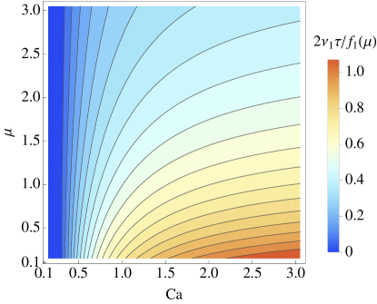
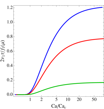
Figure 6: Exponential decay rate of the number of drops for $d=3$ and $\ell=10^{3}$ (a) as a function of $\mu$ and $\mathit{Ca}$ and (b) as a function of the capillary number rescaled by its critical value for fixed $\mu=0.1,1,10$ (from top to bottom).

3.3 Mean lifetime of a drop

The average time it takes for a drop of initial size $r_{0}$ to break can be calculated from $\mathscr{P}(r)$ as follows. Consider the transition probability $p(r,t|r_{0},0)$, which is the solution of (6) that satisfies the initial condition $p(r,0|r_{0},0)=\delta(r-r_{0})$. Let $T(r_{0})$ be the time it takes for the drop to break in a given realization of the flow and of thermal noise, and let $\mathbb{P}(r_{0},t)$ be the probability of $T(r_{0})$ taking the value $t$. Note that $\mathbb{P}(r_{0},t)=-\partial_{t}F$, where $F(r_{0},t)=\int_{t}^{\infty}\mathbb{P}(r_{0},s)\mathrm{d}s$ is the probability that $T(r_{0})\geqslant t$ and can be written as $F(r_{0},t)=\int_{0}^{\ell}p(r,t|r_{0},0)\mathrm{d}r$. Therefore, the average of $T(r_{0})$ is (Gardiner, 1983):

$$\overline{T}(r_{0})=\int_{0}^{\infty}t\,\mathbb{P}(r_{0},t)\mathrm{d}t=-\int_{0}^{\infty}t[\partial_{t}F(r_{0},t)]\mathrm{d}t=\int_{0}^{\infty}F(r_{0},t)\,\mathrm{d}t,$$ (16)

where we used $\lim_{t\to\infty}F(t)=0$, a consequence of the absorbing boundary condition for $p(r,t|r_{0},0)$. By changing the order of integration, we finally obtain:

$$\overline{T}(r_{0})=\int_{0}^{\ell}\mathscr{P}(r)\mathrm{d}r,$$ (17)

where $\mathscr{P}(r)$ is the solution of (8) corresponding to the initial condition $p(r,0)=\delta(r-r_{0})$. Inserting now the asymptotic behaviours (12b) and (13b) into (17) yields:

$${\overline{T}(r_{0})}\sim\begin{cases}\left(\dfrac{\ell}{r_{\mathrm{eq}}}\right)^{\beta-1}-\left(\dfrac{r_{0}}{r_{\mathrm{eq}}}\right)^{\beta-1}&\text{if $\mathit{Ca}<\mathit{Ca}_{c}$},\\[14.22636pt] \ln\bigg{(}\dfrac{\ell}{r_{0}}\bigg{)}&\text{if $\mathit{Ca}>\mathit{Ca}_{c}$},\end{cases}$$ (18)

as seen in figure 5.

4 Improved version of the model of Maffettone & Minale (1998)

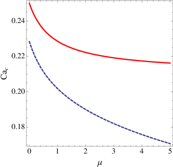
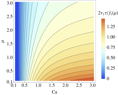
Figure 7: (a) Dependence of the critical capillary number on the viscosity ratio in the original model (red solid curve) and in the improved model (blue dashed curve); (b) Exponential decay rate of the number of drops for $d=3$ and $\ell=10^{3}$ as a function of $\mathit{Ca}$ and $\mu$ for the improved model.

Maffettone & Minale (1998) proposed a modification of their model that improves the agreement with experimental data for high viscosity ratios and large capillary numbers. In the modified model, the coefficient in front of the strain tensor also depends on $\mathit{Ca}$, i.e., $f_{2}(\mu)$ is replaced with

$$\tilde{f}_{2}(\mu,\mathit{Ca})=f_{2}(\mu)+\dfrac{3(\sigma\mathit{Ca})^{2}}{2+6(\sigma\mathit{Ca})^{2}},$$ (19)

where the coefficient $\sigma$ accounts for the fact that here $\mathit{Ca}$ is defined in terms of $\lambda$ (hence in our case $\sigma=1.72$). The above expression still reproduces the theoretical limits, for both small $\mathit{Ca}$ and large $\mu$, as well as the affine deformation of the drop when $\mu=1$ and $\mathit{Ca}\to\infty$. Using $\tilde{f}_{2}$ instead of $f_{2}$ yields significantly more accurate predictions for a pure shear; for an elongational flow, the effect is much weaker (Maffettone & Minale, 1998).

It should be noted that the original model and the improved one can be mapped into each other by suitably modifying the viscosity ratio and the capillary relaxation time. The original model with parameters $\mu$, $\tau$ is indeed the same as the improved one with parameters $\mu^{\prime}$, $\tau^{\prime}$, where $\mu^{\prime}$ and $\tau^{\prime}$ are the solutions of the system:

$$f_{1}(\mu^{\prime})/\tau^{\prime}=f_{1}(\mu)/\tau,\qquad\tilde{f}_{2}(\mu^{\prime},\sigma\lambda\tau^{\prime})=f_{2}(\mu).$$ (20)

Therefore, for fixed $\mu$ and $\mathit{Ca}$, the results described in the previous Sections also hold for the improved model, provided the parameters are suitably adjusted. The reader should note that such a nonlinear transformation of the parameters leads to a slight variation, quantitatively, of the results without changing the overall picture. It is nonetheless important to examine the effect of the modified coefficient $\tilde{f}_{2}$ on quantities such as the critical capillary number, the rate of decay of the drop fraction, and the exponent $\beta$ that defines the power-law behaviour of both the p.d.f. of the size and the mean lifetime. This is achieved by replacing $\gamma(\mu)$ in § 3 with $\tilde{\gamma}(\mu,\mathit{Ca})=\tilde{f}_{2}(\mu,\mathit{Ca})/f_{1}(\mu)$. Thus, the differences between the two versions of the model are mainly due to the fact that $\gamma(\mu)$ varies weakly with $\mu$ and is bounded for $\mu\to\infty$, whereas $\tilde{\gamma}(\mu,\mathit{Ca})\to\infty$ in the same limit. It is shown below that, for a turbulent flow, these differences impact our predictions only marginally.

When the improved model is considered, the critical capillary number is the solution of the cubic equation $\tilde{\gamma}(\mu,\mathit{Ca}_{c})\mathit{Ca}_{c}=1/2$. It can be checked that the discriminant of this equation is negative for all values of $\mu$ and hence there is only one real root. Figure 7(a) compares the critical capillary number in the original model and in the improved one. In both cases, $\mathit{Ca}_{c}$ is a decreasing function of $\mu$. The main difference is that, for $\mu\to\infty$, $\mathit{Ca}_{c}$ tends to the asymptotic value $4/19\approx 0.21$ in the original model, whereas it tends to zero in the improved one. Nevertheless, for the values of $\mu$ typically found in experiments, $\mathit{Ca}_{c}$ does not differ considerably in the two models.

In the improved model, the rate of decay of the number of drops is slightly greater and decreases less rapidly as a function on $\mu$, (compare figures 6(a) and 7(b)). The exponent $\beta$ takes the form $\beta=1-d+d/2\tilde{\gamma}(\mu,\mathit{Ca})\mathit{Ca}$; it is smaller than in the original model and varies more with $\mu$, as a consequence of the different behaviour of $\tilde{\gamma}(\mu,\mathit{Ca})$ (figure 8). Both for $\beta$ and the decay rate, the discrepancies between the two models are, however, small.

In conclusion, despite some quantitative differences, for realistic values of $\mu$ and Ca the qualitative behaviour of the model of Maffettone & Minale (1998) in a turbulent flow is largely insensitive to the use of either $f_{2}(\mu)$ or $\tilde{f}_{2}(\mu,\mathit{Ca})$.

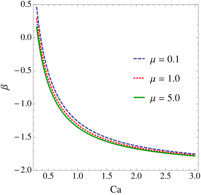
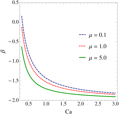
Figure 8: Exponent $\beta$ as a function of the capillary number for $d=3$ (a) in the original model and (b) in the improved model.

5 Conclusions

The Lagrangian dynamics of a sub-Kolmogorov drop in a turbulent flow is determined by the statistics of the velocity gradient. Strong fluctuations of the strain along the trajectory of the drop highly modify the shape and the size of the drop and ultimately break it. We have performed a detailed numerical and analytical study of the deformation and breakup statistics of neutrally buoyant, sub-Kolmogorov, ellipsoidal drops in homogeneous and isotropic turbulence as a function of the capillary number, the viscosity ratio between the inner and outer fluids and the initial drop-size distribution. In particular, we have analytically derived some of the numerical observations reported in Biferale et al. (2014) and have extended the prediction for the critical capillary number to viscosity ratios different from unity. We have also examined further properties of the breakup process, such as the temporal dependence of the number of drops and of the statistics of the size, the role of the initial distribution of the drop sizes, and the mean lifetime of a drop.

Our study relies on the model of Maffettone & Minale (1998). Potential extensions concern the impact on the deformation and breakup dynamics of effects that are not taken into account by this model These include deviations from the ellipsoidal shape, nonlinear deformations near to breakup, large density contrasts between the fluids inside and outside the drop, or secondary breakups. More refined models of drop dynamics have indeed been proposed in the literature (e.g. Minale, 2010). However, such models generally depend in a highly nonlinear way on the shape of the drop, and this renders their analytical study very challenging.

It would also be interesting to understand possible intermittency effects for such sub-Kolmogorov scale droplets (Biferale, Meneveau & Verzicco, 2014) (and also studied for larger droplets (Perlekar et al., 2012)) and if there are analogues of transparency effects, seen in oscillatory, laminar flows (Milan et al., 2018) for droplets in fully developed turbulence.

Finally, Maffettone & Minale (1998) observe that, for $\mu=1$, their model is closely related to the Oldroyd-B model for solutions of flexible polymers (Bird et al., 1987). Likewise, when $\mu=1$ and hence $\mathsfbi{G}=\bnabla\bm{u}$ the vector model of Olbricht et al. (1982) reduces to the Hookean dumbbell model, which describes the evolution of the end-to-end separation vector of a flexible polymer molecule in the limit in which nonlinear elastic effects are negligible (Bird et al., 1987). Therefore, after appropriate redefinition of the parameters, our results also apply to the degradation of polymers in turbulent flows.

Appendix A Cholesky decomposition of the tensor $\mathsfbi{M}$

The Cholesky decomposition of $\mathsfbi{M}$ is $\mathsfbi{M}=\mathsfbi{L}\mathsfbi{L}^{\top}$, where $\mathsfbi{L}$ is a lower triangular matrix. The elements of $\mathsfbi{L}$ satisfy:

$$\dot{L}_{11} = G_{11}L_{11}+G_{12}L_{21}+G_{13}L_{31}+c_{\tau}\left[\dfrac{c_{g}}{L_{11}}-L_{11}\right]$$

$$\dot{L}_{21} = G_{21}L_{11}+G_{22}L_{21}+G_{23}L_{31}+G_{12}\dfrac{L_{22}^{2}}{L_{11}}+G_{13}\dfrac{L_{32}L_{22}}{L_{11}}-c_{\tau}\left[L_{21}+c_{g}\dfrac{L_{21}}{L_{11}^{2}}\right]$$

$$\dot{L}_{31} = G_{31}L_{11}+G_{32}L_{21}+G_{33}L_{31}+G_{12}\dfrac{L_{22}L_{32}}{L_{11}}+G_{13}\dfrac{L_{32}^{2}+L_{33}^{2}}{L_{11}}-c_{\tau}\left[L_{31}+c_{g}\dfrac{L_{31}}{L_{11}^{2}}\right]$$

$$\dot{L}_{22} = G_{22}L_{22}+G_{23}L_{32}-G_{12}\dfrac{L_{21}L_{22}}{L_{11}}-G_{13}\dfrac{L_{32}L_{21}}{L_{11}}+c_{\tau}\left[-L_{22}+\dfrac{c_{g}}{L_{22}}+c_{g}\dfrac{L_{21}^{2}}{L_{11}^{2}L_{22}}\right]$$

$$\dot{L}_{32} = G_{32}L_{22}+G_{33}L_{32}-G_{12}\dfrac{L_{22}L_{31}}{L_{11}}-G_{13}\dfrac{L_{31}L_{32}}{L_{11}}+G_{23}\dfrac{L_{33}^{2}}{L_{22}}-G_{13}\dfrac{L_{21}L_{33}^{2}}{L_{11}L_{22}}$$

$$+2c_{\tau}c_{g}\dfrac{L_{21}L_{31}}{L_{11}^{2}L_{22}}+c_{\tau}\left[-L_{32}-c_{g}\dfrac{L_{32}}{L_{22}^{2}}-c_{g}\dfrac{L_{21}^{2}L_{32}}{L_{11}^{2}L_{22}^{2}}\right]$$

$$\dot{L}_{33} = G_{33}L_{33}-G_{13}\dfrac{L_{31}L_{33}}{L_{11}}-G_{23}\dfrac{L_{32}L_{33}}{L_{22}}+G_{13}\dfrac{L_{21}L_{32}L_{33}}{L_{11}L_{22}}-2c_{\tau}c_{g}\dfrac{L_{21}L_{31}L_{32}}{L_{11}^{2}L_{22}L_{33}}$$

$$+c_{\tau}\left[-L_{33}+\dfrac{c_{g}}{L_{33}}+c_{g}\dfrac{L_{31}^{2}}{L_{11}^{2}L_{33}}+c_{g}\dfrac{L_{32}^{2}}{L_{22}^{2}L_{33}}+c_{g}\dfrac{L_{21}^{2}L_{32}^{2}}{L_{11}^{2}L_{22}^{2}L_{33}}\right]$$

with $c_{\tau}=f_{1}(\mu)/2\tau$ and $c_{g}=g(\mathsfbi{L}\mathsfbi{L}^{\top})$ (the functions $f_{1}$ and $g$ are defined after (1)). The above equations can be derived by adapting to (1) the equations obtained in Vaithianathan & Collins (2003) for a constitutive model of viscoelastic fluid (see also Perlekar, Mitra & Pandit (2006), where a misprint is corrected in the equation for $L_{32}$). The positivity of $L_{ii}$, $i=1,2,3$, is enforced by evolving $\ln L_{ii}$ instead of $L_{ii}$ (Vaithianathan & Collins, 2003).

References

- Ayyalasomayajula, Collins & Warhaft (2008) Ayyalasomayajula, S., Collins, L. R. & Warhaft, Z. 2008 Modeling inertial particle acceleration statistics in isotropic turbulence. Phys. Fluids 20, 095104.
- Ayyalasomayajula, Gylfason & Warhaft (2008) Ayyalasomayajula, S., Gylfason, A. & Warhaft, Z. 2008 Lagrangian measurements of fluid and inertial particles in decaying grid generated turbulence, in IUTAM Symposium on Computational Physics and New Perspectives in Turbulence, Nagoya, Japan, Y. Kaneda (ed.) (IUTAM Bookseries, vol. IV, pp. 171–175).
- Balkovsky, Fouxon & Lebedev (2001) Balkovsky, E., Fouxon, A. & Lebedev, V. (2001) Turbulence of polymer solutions. Phys. Rev. E 64, 056301.
- Bec et al. (2006) Bec, J., Biferale, L., Boffetta, G., Cencini, M., Lanotte, A., Musacchio, S. & Toschi, F. 2006 Lyapunov exponents of heavy particles in turbulence. Phys. Fluids 18, 091702.
- Biferale, Meneveau & Verzicco (2014) Biferale, L., Meneveau, C. & Verzicco, R. 2014 Deformation statistics of sub-Kolmogorov-scale ellipsoidal neutrally buoyant drops in isotropic turbulence. J. Fluid Mech. 754, 184–207.
- Bird et al. (1987) Bird, R. B., Hassager, O., Armstrong, R. C. & Curtiss, C. F. 1987 Dynamics of Polymeric Liquids, vol. II. Wiley.
- Brunk & Koch (1998) Brunk, B. K. & Koch, D. L. (1997) Hydrodynamic pair diffusion in isotropic random velocity fields with application to turbulent coagulation. Phys. Fluids 9, 2670.
- Celani, Musacchio & Vincenzi (2005) Celani, A., Musacchio, S. & Vincenzi, D. 2005 Polymer transport in random flow. J. Stat. Phys. 118, 531–554.
- Cristini et al. (2003) Cristini, V., Bławzdziewicz, J., Loewenberg, M. & Collins, L. R. 2003 Breakup in stochastic Stokes flows: sub-Kolmogorov drops in isotropic turbulence. J. Fluid Mech. 492, 231–250.
- Falkovich, Gawȩdzki & Vergassola (2001) Falkovich, G., Gawȩdzki, K. & Vergassola, M. (2001) Particles and fields in fluid turbulence. Rev. Mod. Phys. 73, 913–975.
- Gardiner (1983) Gardiner, C. W. 1983 Handbook of Stochastic Methods. Springer.
- Girimaji & Pope (1990) Girimaji, S. S. & Pope, S. B. 1990 A diffusion model for velocity gradients in turbulence. Phys. Fluids A 2, 242–256.
- Hinze (1955) Hinze, J. O. 1955 Fundamentals of the hydrodynamic mechanism of splitting in dispersion processes. AIChE J. 1, 289–295.
- James & Ray (2017) James, M. & Ray, S. S. 2017 Enhanced droplet collision rates and impact velocities in turbulent flows: The effect of polydispersity and transient phases. Sci. Rep. 7, 12231.
- Kolmogorov (1949) Kolmogorov, A. N. 1949 On the breakage of drops in a turbulent flow. Dokl. Akad. Nauk SSSR 66, 825–828. [For the English translation, see V.M. Tikhomiro (ed.), Selected Works of A.N. Kolmogorov (Kluwer Academic Publishers, 1991), pp. 339–343].
- Le Jan (1984) Le Jan, Y. 1984 Exposants de Lyapunov pour les mouvements browniens isotropes. C. R. Acad. Sci. Paris Ser. I 299, 947–949.
- Le Jan (1985) Le Jan, Y. 1985 On isotropic Brownian motions. Z. Wahrscheinlichkeitstheor. verw. Gebiete 70, 609–620.