Greybody factor of scalar fields from black strings

Abstract

The greybody factor of massless, uncharged scalar fields is studied in the background of cylindrically symmetric spacetimes, in the low-energy approximation. We discuss two cases. In the first case we derive analytical expression for the absorption probability when the spacetime is kinetically coupled with the Einstein tensor. In the second case we do the analysis in the absence of the coupling constant. For this purpose we analyze the wave equation which is obtained from Klein-Gordon equation. The radial part of the wave equation is solved in the form of the hypergeometric function in the near horizon region, whereas in the far region the solution is of the form of Bessel’s function. Finally, considering continuity of the wave function we smoothly match the two solutions in the low energy approximation to get the formula for the absorption probability.

Key Words: Greybody factor; Matching technique; Low energy regime

1 Introduction

Black holes are the most interesting objects worth investigating in any gravitational theory. Considering black holes as thermal systems their entropy and thermodynamics were investigated by taking into account quantum mechanical effects JBS ; J . Thus black holes have an associated temperature and entropy and therefore they radiate, and the radiations are called Hawking radiations. Hawking temperature of radiations emitted from different black holes has been studied UK ; MK ; AK1 . The emission rate at the event horizon of a black hole, in a mode with frequency $\omega$, is given by SW

$$\Gamma(\omega)=\left(\frac{1d^{3}k}{e^{\beta\omega}\pm 1(2\pi)^{3}}\right),$$ (1)

where $\beta$ is the inverse of Hawking temperature and the minus (plus) sign is for bosons (fermions). This formula for the emission rate can be generalized for any dimension and it is valid for massive and massless particles. Therefore at the event horizon the spectrum of the radiations from black holes is perfectly the same as that of the black-body spectrum. Due to this it gives rise to the information loss paradox. The important fact is that geometry of the spacetime around a black is non-trivial. This non-trivial geometry modifies the spectrum of Hawking radiations. In fact the non-trivial geometry acts as a potential barrier which allows some of the radiations to transmit and to reflect the rest to the hole.

The greybody factor, defined as the probability for a given wave coming from infinity to be absorbed by the black hole (rate of absorption probability), is directly connected to the absorption cross section YH ; TJ ; JAKS ; JAS ; AFB ; SI ; IS ; MF ; WJ ; L1 . The mathematical expression that summarizes the above discussion is

$$\Gamma(\omega)=\left(\frac{\gamma(\omega)d^{3}k}{e^{\beta\omega}\pm 1(2\pi)^{3}}\right),$$ (2)

where $\gamma(\omega)$ is the so-called greybody factor, which is frequency dependent.

Physically the greybody factor originates from an effective potential barrier by a black hole spacetime. For example the potential barrier for massless scalars from Schwarzschild spacetime is

$$V_{eff}\left(x\right)=\left(1-\frac{r_{H}}{r}\right)\left(\frac{r_{H}}{r^{3}}+\frac{l(l+1)}{r^{2}}\right),$$ (3)

with the tortoise coordinate

$$x=r+r_{H}\ln\left(\frac{r}{r_{H}}-1\right),$$ (4)

where $r_{H}$ is the horizon radius and $l$ is the angular momentum of the scalar. It is this potential which transmits or reflects radiations from black holes. Therefore it gives rise to the frequency dependent greybody factor. This factor not only accounts for the deviation of Hawking radiations from the black-body spectrum, but it also could be important in the energy emission rate and relevant to compute the partial absorption cross section of black holes. The main idea to obtain the expression for the greybody factor is to derive the solution of the relevant wave equation in near horizon and asymptotic regions separately and then match them to an appropriate intermediate point JAS ; AFB ; SI ; IS ; MF ; WJ ; D ; W ; PJA .

Scalar fields, non-minimally coupled with gravity, have shown significant features, both for inflation and dark energy. Also, the non-minimal couplings between derivatives of the scalar fields and the curvature reveal interesting cosmological behaviours. In general, the scalar-tensor theories give both the Einstein equation and the equation of motion for the scalar in the form of fourth-order differential equations. But if the kinetic term is only coupled to the Einstein tensor, the equation of motion for scalars is reduced to a second-order differential equation. Therefore, from the point of view of physics, considering such a coupling can be interpreted as a good theory because it is very simple. In the light of the earlier results G11 ; G12 ; SS11 there is a need for more efforts to be focussed on the study of scalar fields coupled with tensors for more general cases. In order to fill the gap in the literature, for the case of cylindrically symmetric black holes, we have studied the properties of the scalar field when it is kinetically coupled to the Einstein tensor and the one without any coupling, separately.

The rest of this letter is organized as follows. In Section 2 Klein-Gordon equation in a charged black string background with coupling to the Einstein tensor is given. In Section 3 solutions of the radial equation resulting from the Klein-Gordon equation in the near horizon region and the far horizon regime are presented. These are also matched to an intermediate region to get a value of the absorption probability. In Section 4 we do the above analysis in the absence of the coupling parameter. Section 5 gives some concluding remarks.

2 Klein-Gordon equation in the background of charged black string

The Klein Gordon equation when the Einstein tensor is coupled to a massless, uncharged scalar field is

$$\frac{1}{\sqrt{-g}}\partial_{\mu}\Big{[}\sqrt{-g}\left(g^{\mu\nu}+\eta\epsilon^{\mu\nu}\right)\partial_{\nu}\Psi\Big{]}=0,$$ (5)

where $\eta$ is a coupling constant and $\epsilon^{\mu\nu}$ is Einstein’s tensor. The charged black string having non-zero components of Einstein’s tensor is JK

$$ds^{2}=-f(r)dt^{2}+\frac{1}{f(r)}dr^{2}+r^{2}d\theta^{2}+\alpha^{2}r^{2}dz^{2},$$ (6)

where

$$f(r)=\alpha^{2}r^{2}-\frac{4M}{\alpha r}+\frac{4Q^{2}}{\alpha^{2}r^{2}}.$$ (7)

Here $M$ is the mass, $Q$ is the charge and $\alpha=-\Lambda/3$, with $\Lambda$ being the cosmological constant. For the above metric the Einstein tensor $\epsilon^{\mu\nu}$ in matrix form can be written as

$$\epsilon^{\mu\nu}=\frac{4Q^{2}}{\alpha^{4}r^{4}}\left(\begin{array}[]{cccc}-\frac{1}{f}&0&0&0\\ 0&f&0&0\\ 0&0&-\frac{1}{r^{2}}&0\\ 0&0&0&-\frac{1}{\alpha^{2}r^{2}}\end{array}\right).$$ (8)

Also

$$\sqrt{-g}=\alpha r^{2}.$$ (9)

Substituting the components of the Einstein tensor and spacetime metric in equation (5), it takes the form

$$\frac{1}{\alpha r^{2}}\partial_{t}\bigg{[}\alpha r^{2}\left(-\frac{1}{f}-\frac{4\eta Q^{2}}{\alpha^{4}r^{4}f}\right)\partial_{t}\Psi\bigg{]}+\frac{1}{\alpha r^{2}}\partial_{r}\bigg{[}\alpha r^{2}\left(f+\frac{4\eta Q^{2}f}{\alpha^{4}r^{4}}\right)\partial_{r}\Psi\bigg{]}+$$

$$\frac{1}{\alpha r^{2}}\partial_{\theta}\bigg{[}\alpha r^{2}\left(\frac{1}{r^{2}}-\frac{4\eta Q^{2}}{\alpha^{4}r^{6}}\right)\partial_{\theta}\Psi\bigg{]}+\frac{1}{\alpha r^{2}}\partial_{z}\bigg{[}\alpha r^{2}\left(\frac{1}{\alpha r^{2}}-\frac{4\eta Q^{2}}{\alpha^{6}r^{6}}\right)\partial_{\theta}\Psi\bigg{]}=0.$$ (10)

Using the form of cylindrical harmonics

$$\Psi(t,r,\theta,z)=e^{-\iota\omega t}R(r)Y(\theta,z),$$ (11)

we get from the radial part of equation $\left(\ref{15}\right)$ as

$$\frac{1}{r^{2}}\frac{d}{dr}\bigg{[}r^{2}\left(1+\frac{4\eta Q^{2}}{\alpha^{4}r^{4}}\right)f\bigg{]}\frac{dR(r)}{dr}+\left[\left(1+\frac{4\eta Q^{2}}{\alpha^{4}r^{4}}\right)\frac{\omega^{2}}{f}-\left(1-\frac{4\eta Q^{2}}{\alpha^{4}r^{4}}\right)\frac{F_{lm}}{\alpha^{2}r^{2}}\right]R(r)=0,$$ (12)

where $F_{lm}=l(l+1)$ are the eigenvalues coming from the $(\theta,z)$ part.

3 Greybody factor computation

3.1 Near horizon solution

Equation $\left(\ref{17}\right)$ is the master equation of our interest. We will solve this equation in two regions separately, namely, the near horizon region and the far region by using a semi-classical approach known as the simple matching technique. We will match both solutions to an intermediate region to get the analytical expression for the absorption probability.

For the near horizon region $r\sim r_{+}$, we will perform the following transformation to simplify the radial equation SOPK ; DKS :

$$r\rightarrow f,$$ (13)

which implies

$$\frac{df}{dr}=\left(1-f\right)\frac{B(r_{+})}{r_{+}},$$ (14)

where $r_{+}$ is the horizon and

$$B(r_{+})=1-\frac{4Q^{2}-2\alpha^{4}r_{+}^{4}}{4M\alpha r_{+}-4Q^{2}}.$$ (15)

Using the above, equation $\left(\ref{17}\right)$ takes the form

$$f(1-f)\frac{d^{2}R(f)}{df^{2}}+\left(1-C_{\ast}f\right)\frac{dR(f)}{df}$$

$$+\left[\frac{F_{\ast}^{2}}{B^{2}(r_{+})\left(1-f\right)f}-\left(\frac{\alpha^{4}r_{+}^{4}-4\eta Q^{2}}{\alpha^{4}r_{+}^{4}+4\eta Q^{2}}\right)\frac{F_{lm}}{B^{2}(r_{+})\alpha^{2}\left(1-f\right)}\right]R(f)=0.$$ (16)

Here

$$F_{\ast}=\omega r_{\ast},$$ (17)

and

$$C_{\ast}=2-\frac{2}{B(r_{+})}\left(\frac{\alpha^{4}r_{+}^{4}-4\eta Q^{2}}{\alpha^{4}r_{+}^{4}+4\eta Q^{2}}\right).$$ (18)

In order to further simplify the above equation, we use the field redefinition

$$R(f)=f^{\mu}\left(1-f\right)^{\nu}F(f).$$ (19)

Using this in equation $\left(\ref{21}\right)$, we obtain

$$f\left(1-f\right)\frac{d^{2}F(f)}{df^{2}}+\left[1+2\mu-\left(2\mu+2\nu+C_{\ast}\right)f\right]\frac{dF}{df}$$

$$+[\frac{\mu^{2}}{f}-\mu^{2}+\mu-2\mu\nu+\frac{\nu^{2}}{1-f}-\nu^{2}-\frac{2\nu}{1-f}+\nu-\mu C_{\ast}+\frac{\nu C_{\ast}}{1-f}-\nu C_{\ast}$$

$$+\frac{F_{\ast}^{2}}{B^{2}(r_{+})f}+\frac{F_{\ast}^{2}}{B^{2}(r_{+})\left(1-f\right)}-\left(\frac{\alpha^{4}r_{+}^{4}-4\eta Q^{2}}{\alpha^{4}r_{+}^{4}+4\eta Q^{2}}\right)\frac{F_{lm}}{B^{2}(r_{+})\alpha^{2}\left(1-f\right)}]F(f)=0.$$ (20)

We define

$$a=\mu+\nu+C_{\ast}-1,\,\,\ b=\mu+\nu,\,\,\ c=1+2\mu.$$ (21)

Also the constraints coming from the coefficients of $F(f)$ give

$$\mu^{2}+\frac{F_{\ast}^{2}}{B^{2}(r_{+})}=0,$$ (22)

and

$$\nu^{2}+\nu(C_{\ast}-2)+\frac{F_{\ast}^{2}}{B^{2}(r_{+})}-\left(\frac{\alpha^{4}r_{+}^{4}-4\eta Q^{2}}{\alpha^{4}r_{+}^{4}+4\eta Q^{2}}\right)\frac{F_{lm}}{B^{2}(r_{+})\alpha^{2}}=0.$$ (23)

From this we get the values of $\mu$ and $\nu$:

$$\mu_{\pm}=\pm\iota\frac{F_{\ast}}{B(r_{+})},$$ (24)

and

$$\nu_{\pm}=\frac{1}{2}\left[\left(2-C_{\ast}\right)\pm\sqrt{\left(2-C_{\ast}\right)^{2}-4\left(\frac{F_{\ast}^{2}}{B^{2}(r_{+})}-\left(\frac{\alpha^{4}r_{+}^{4}-4\eta Q^{2}}{\alpha^{4}r_{+}^{4}+4\eta Q^{2}}\right)\frac{F_{lm}}{B^{2}(r_{+})\alpha^{2}}\right)}\right].$$ (25)

Equation $\left(\ref{25}\right)$ by virtue of $\left(\ref{26}\right)$ and the constraints $\left(\ref{27}\right)$-$\left(\ref{28}\right)$ becomes

$$f\left(1-f\right)\frac{d^{2}F(f)}{df^{2}}+\bigg{[}c-\left(1+a+b\right)f\bigg{]}\frac{dF(f)}{df}-abF(f)=0.$$ (26)

For the near horizon case there exists no outgoing mode, which means $\mu_{+}=\mu_{-}$ and $\nu_{+}=\nu_{-}$. So in the near horizon region the solution can be written in the form of the general hypergeometric function, which has the form

$$R(f)_{NH}=C_{-}f^{\mu}(1-f)^{\nu}F\left(a,b,c;f\right),$$ (27)

where $C_{-\text{ }}$ is an arbitrary constant.

3.2 Far horizon solution

Now we find the solution of the radial equation for the far region. In this case the radial part will have the form

$$\frac{d^{2}R(r)_{FR}}{dr^{2}}+\frac{4}{r}\frac{dR(r)_{FR}}{dr}+\left(\omega^{2}-\frac{F_{lm}}{\alpha^{2}r^{2}}\right)R(r)_{FR}=0.$$ (28)

This is the well-known Bessel equation, and in a far field its solution can be written as

$$R_{FR}\left(r\right)=\frac{1}{\sqrt{r\alpha\omega}}\left[B_{1}J_{\gamma}(\omega\alpha r)+B_{2}Y_{\gamma}(\omega\alpha r)\right].$$ (29)

In the above solution $J_{\gamma}$ and $Y_{\gamma}$ are Bessel’s functions. For $\gamma=l+1/2$, and in the limit $r\rightarrow 0$, the above solution can be written as

$$R_{FR}\left(r\right)\simeq\frac{B_{1}\left(\frac{\omega\alpha r}{4}\right)^{\gamma}}{\sqrt{\omega\alpha r}\Gamma\left(\nu+1\right)}-\frac{B_{2}\Gamma\left(\gamma\right)}{\pi\sqrt{\omega\alpha r}\left(\frac{\omega\alpha r}{4}\right)^{\nu}}.$$ (30)

3.3 Matching the two solutions

We now stretch the near horizon solution to an intermediate region SJ ; MI which gives

$$R(f)_{NH}=C_{-}f^{\mu}\left(1-f\right)^{\nu}\bigg{[}\frac{\Gamma(c)\Gamma(c-a-b)}{\Gamma(c-a)\Gamma(c-b)}F\left(a,b,a+b-c+1;1-f\right)$$

$$+\left(1-f\right)^{c-a-b}\frac{\Gamma(c)\Gamma(a+b-c)}{\Gamma(a)\Gamma(b)}F\left(c-a,c-b,c-a-b+1;1-f\right)\bigg{]}.$$ (31)

We can approximate $1-f$ for the case $r\gg r_{+}$ as

$$1-f\simeq\frac{4M}{\alpha r}.$$ (32)

So, the form of the final solution for the near horizon case becomes

$$R(r)_{NH}\simeq A_{1}r^{\nu}+A_{2}r^{-(\nu+C_{\ast}-2)}.$$ (33)

Here we have chosen

$$A_{1}=C_{-}\left(\frac{4M}{\alpha}\right)^{\nu}\frac{\Gamma(c)\Gamma(c-a-b)}{\Gamma(c-a)\Gamma(c-b)},$$ (34)

and

$$A_{2}=C_{-}\left(\frac{4M}{\alpha}\right)^{-(\nu+C_{\ast}-2)}\frac{\Gamma(c)\Gamma(a+b-c)}{\Gamma(a)\Gamma(b)}.$$ (35)

In the low-energy limit we can use the approximation

$$-\nu\simeq l+O(\omega^{2}),$$ (36)

$$\nu+C_{\ast}-2\simeq-\left(l+1\right)+O(\omega^{2}).$$ (37)

From equations $\left(\ref{35}\right)$ and $\left(\ref{40}\right)$ matching the coefficients and eliminating $C_{-}$ give

$$B=\frac{B_{1}}{B_{2}}=-\frac{1}{\pi}\frac{1}{\left(\alpha\omega M\right)^{2l+1}}\frac{\Gamma(c-a-b)\Gamma(a)\Gamma(b)}{\Gamma(c-a)\Gamma(c-b)\Gamma(a)\Gamma(b)}\Gamma^{2}(l+1/2).$$ (38)

The greybody factor can now be given by LAEJ

$$\gamma_{l}\left(\omega\right)=\left|P_{l}\right|^{2}=\frac{2\iota\left(B^{\ast}-B\right)}{\left|B\right|^{2}}.$$ (39)

By using the value of $B$ we can find the expression of absorption probability of the radiations emitted from the charged black string. This relation gives a measure of how much the radiations are different (or modified) from the spectrum of the black body radiation.

4 Absorption probability for scalar field without coupling to the Einstein tensor

In this section we find an analytical expression of the absorption probability for scalar field from the charged black string without coupling to the Einstein tensor. The Klein-Gordon equation for a massless, uncharged scalar field is

$$\frac{1}{\sqrt{-g}}\partial_{\mu}\left[\sqrt{-g}\left(g^{\mu\nu}\right)\partial_{\nu}\Psi\right]=0.$$ (40)

Using the values of each component of the spacetime considered in the previous section, we get the following equation:

$$\frac{1}{\alpha r^{2}}\partial_{t}\bigg{[}\alpha r^{2}\left(-\frac{1}{f}\right)\partial_{t}\Psi\bigg{]}+\frac{1}{\alpha r^{2}}\partial_{r}\bigg{[}\alpha r^{2}\left(f\right)\partial_{r}\Psi\bigg{]}+$$

$$\frac{1}{\alpha r^{2}}\partial_{\theta}\bigg{[}\alpha r^{2}\left(\frac{1}{r^{2}}\right)\partial_{\theta}\Psi\bigg{]}+\frac{1}{\alpha r^{2}}\partial_{z}\bigg{[}\alpha r^{2}\left(\frac{1}{\alpha r^{2}}\right)\partial_{\theta}\Psi\bigg{]}=0.$$ (41)

Considering cylindrical harmonics, we can separate the radial part of equation $\left(\ref{2a}\right)$, which has the form

$$\frac{1}{\alpha r^{2}}\frac{d}{dr}\left(\alpha r^{2}f\right)\frac{dR(r)}{dr}+\left[\frac{\omega^{2}}{f}-\frac{F_{lm}}{\alpha^{2}r^{2}}\right]R(r)=0.$$ (42)

As in the previous case we will find two solutions of the radial equation $\left(\ref{3a}\right)$, one for the near horizon and the other for the far horizon regime. In the case of the near horizon region, we use the transformation $r\rightarrow f$, which implies

$$\frac{df}{dr}=\left(1-f\right)\frac{B(r_{+})}{r_{+}},$$ (43)

where

$$B(r_{+})=1-\frac{4Q^{2}-2\alpha^{4}r_{+}^{4}}{4M\alpha r_{+}-4Q^{2}}.$$ (44)

Using equation $\left(\ref{5a}\right)$, equation $(\ref{3a})$ takes the form

$$f(1-f)\frac{d^{2}R(f)}{df^{2}}+\left(1-C_{\ast}f\right)\frac{dR(f)}{df}+\left[\frac{F_{\ast}^{2}}{B^{2}(r_{+})\left(1-f\right)f}-\frac{F_{lm}}{B^{2}(r_{+})\alpha^{2}\left(1-f\right)}\right]R(f)=0.$$ (45)

Here

$$F_{\ast}=\omega r_{\ast},\,\,\,\ C_{\ast}=2-\frac{2}{B(r_{+})}.$$ (46)

In order to further simplify the above equation, we use field redefinition

$$R(f)=f^{\mu}\left(1-f\right)^{\nu}F(f).$$ (47)

In equation $\left(\ref{7a}\right)$ we use this definition of $R(f)$ to obtain

$$f\left(1-f\right)\frac{d^{2}F(f)}{df^{2}}+\bigg{[}1+2\mu-\left(2\mu+2\nu+C_{\ast}\right)f\bigg{]}\frac{dF}{df}+$$

$$\bigg{[}\frac{\mu^{2}}{f}-\mu^{2}+\mu-2\mu\nu+\frac{\nu^{2}}{1-f}-\nu^{2}-\frac{2\nu}{1-f}+\nu-\mu C_{\ast}+\frac{\nu C_{\ast}}{1-f}-\nu C_{\ast}+$$

$$\frac{F_{\ast}^{2}}{B^{2}(r_{+})f}+\frac{F_{\ast}^{2}}{B^{2}(r_{+})\left(1-f\right)}-\left(\frac{\alpha^{4}r_{+}^{4}-4\eta Q^{2}}{\alpha^{4}r_{+}^{4}+4\eta Q^{2}}\right)\frac{F_{lm}}{B^{2}(r_{+})\alpha^{2}\left(1-f\right)}\bigg{]}F(f)=0.$$ (48)

We again use the definitions given in (21). The constraints coming from the coefficients of $F(f)$ yield

$$\mu^{2}+\frac{F_{\ast}^{2}}{B^{2}(r_{+})}=0,$$ (49)

and

$$\nu^{2}+\nu(C_{\ast}-2)+\frac{F_{\ast}^{2}}{B^{2}(r_{+})}-\frac{F_{lm}}{B^{2}(r_{+})\alpha^{2}}=0.$$ (50)

These give the values of $\mu$ and $\nu$ as

$$\mu_{\pm}=\pm\iota\frac{F_{\ast}}{B(r_{+})},$$ (51)

$$\nu_{\pm}=\frac{1}{2}\left[\left(2-C_{\ast}\right)\pm\sqrt{\left(2-C_{\ast}\right)^{2}-4\left(\frac{F_{\ast}^{2}}{B^{2}(r_{+})}-\frac{F_{lm}}{B^{2}(r_{+})\alpha^{2}}\right)}\right].$$ (52)

Equation $\left(\ref{11a}\right)$ by virtue of the above constraints becomes

$$f\left(1-f\right)\frac{d^{2}F(f)}{df^{2}}+\bigg{[}c-\left(1+a+b\right)f\bigg{]}\frac{dF(f)}{df}-abF(f)=0.$$ (53)

For the near horizon case there exists no outgoing mode, which means $\mu_{+}=\mu_{-}$ and $\nu_{+}=\nu_{-}$. So, in the near horizon region the solution can be written in the form of the general hypergeometric function, being of the form

$$R(f)_{NH}=C_{1-}f^{\mu}(1-f)^{\nu}F\left(a,b,c;f\right),$$ (54)

where $C_{1-}$ is an arbitrary constant. We now stretch the near horizon solution to an intermediate region SJ ; MI so that

$$R(f)_{NH}=C_{-}f^{\mu}\left(1-f\right)^{\nu}\bigg{[}\frac{\Gamma(c)\Gamma(c-a-b)}{\Gamma(c-a)\Gamma(c-b)}F\left(a,b,a+b-c+1;1-f\right)+$$

$$\left(1-f\right)^{c-a-b}\frac{\Gamma(c)\Gamma(a+b-c)}{\Gamma(a)\Gamma(b)}F\left(c-a,c-b,c-a-b+1;1-f\right)\bigg{]}.$$ (55)

We again approximate $1-f$ for the case $r\gg r_{+}$, as before, and obtain the final form of the solution given in (33).

Now, as in the previous section, the radial equation for the far region reduces to the form of Bessel’s equation, and the form of the final solution in this region is

$$R_{FR}\left(r\right)\simeq\frac{B_{1}\left(\frac{\omega\alpha r}{4}\right)^{\gamma}}{\sqrt{\omega\alpha r}\Gamma\left(\nu+1\right)}-\frac{B_{2}\Gamma\left(\gamma\right)}{\pi\sqrt{\omega\alpha r}\left(\frac{\omega\alpha r}{4}\right)^{\nu}}.$$ (56)

Using the same procedure as in the previous case, we find

$$B=\frac{B_{1}}{B_{2}}=-\frac{1}{\pi}\frac{1}{\left(\alpha\omega M\right)^{2l+1}}\frac{\Gamma(c-a-b)\Gamma(a)\Gamma(b)}{\Gamma(c-a)\Gamma(c-b)\Gamma(a)\Gamma(b)}\Gamma^{2}(l+1/2).$$ (57)

The absorption probability and hence greybody factor can be found by using the value of $B$ in equation $\left(\ref{43}\right)$.

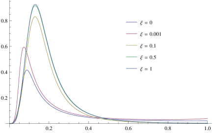
Figure 1: Greybody factor as a function of the frequency, for $\xi=0,0.001,0.1,0.5,1$ and $l=1$

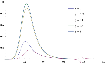
Figure 2: Greybody factor as a function of the frequency, for $\xi=0,0.001,0.1,0.5,1$ and $l=2$

The effect of the coupling constant on the greybody factor is also analyzed graphically for different partial modes. In Fig. 1, we draw the graph of the greybody factor as a function of the frequency for different values of the coupling constant and for $l=1$. In Fig. 2 it is depicted for $l=2$. It is observed that, for different modes, a stronger coupling enhances the absorption probability in the low frequency approximation.

5 Conclusion

In this letter we have studied the greybody factor for a scalar field coupling to the Einstein tensor in the background of a charged black string in the low energy approximation. We found that the absorption probability and hence the greybody factor depend on the coupling between the scalar field and the Einstein tensor. It is observed that the presence of a coupling enhances the absorption probability of the scalar field in the black string spacetime. Also, for weaker coupling, the absorption probability decreases with the increase in the charge of black string. In the second case we did this analysis without considering a coupling of the scalar field and the Einstein tensor. Needless to say that the latter case reduces to the result of the former in the absence of the coupling constant.

References

• (1) J. M. Bardeen, B. Carter and S. Hawking, Commun. Math. Phys. 31 (1973) 161.
• (2) J. D. Bekenstein, Phys. Rev. D 7 (1973) 2333.
• (3) M. K. Parikh and F. Wilczek, Phys. Rev. Lett. 85 (2000) 5042.
• (4) R. Kerner and R. B. Mann, Class. Quantum Grav. 25: 095014 (2008).
• (5) A. Ejaz, H. Gohar, H. Lin, K. Saifullah and S-T. Yau, Phys. Lett. B 726 (2013) 827.
• (6) S. W. Hawking, Commun. Math. Phys. 43 (1975) 199.
• (7) J. M. Maldacena and A. Strominger, Phys. Rev. D 55 (1997) 861.
• (8) I. R. Klebanov and S. D. Mathur, Nucl. Phys. B 500 (1997) 115.
• (9) J. Ahmad and K. Saifullah, Greybody factor of scalar field from Reissner-Nordstrom-de Sitter black hole, arXiv:1610.06104 [gr-qc].
• (10) Y. S. Myung and H. W. Lee, Class. Quantum Grav. 20 (2003) 3533.
• (11) T. Harmark, J. Natario and R. Schiapa, Adv. Theor. Math. Phys. 14 (2010) 727.
• (12) P. R. Anderson, A. Fabbri and R. Balbinot, Phys. Rev. D 91 (2015) 064061.
• (13) S. S. Gubserv and I. R. Klebanov, Phys. Rev. Lett. 77 (1996) 4491.
• (14) M. Cvetic and F. Larsen, Phys. Rev. D 56 (1997) 4994.
• (15) W. T. Kim and J. J. Oh, Phys. Lett. B 461 (1999) 189.
• (16) L. H. Ford, Phys. Rev. D 12 (1975) 2963.
• (17) W. G. Unruh, Phys. Rev. D 14 (1976) 3251.
• (18) D. N. Page, Phys. Rev. D 13 (1976) 198.
• (19) P. Kanti, J. Grain and A. Barrau, Phys. Rev. D 71 (2005) 104002.
• (20) C. J. Gao, JCAP 06 (2010) 023.
• (21) L. N. Granda, JCAP 07 (2010) 006.
• (22) E. N. Saridavis and S. V. Sushkov, Phys. Rev. D 81 (2010) 083510.
• (23) J. Ahmad and K. Saifullah, JCAP 11 (2011) 23.
• (24) S. Creek, O. Efthimiou, P. Kanti and K. Tamvakis, Phys. Rev. D 75 (2007) 084043.
• (25) D. Ida, K. Oda and S. C. Park, Phys. Rev. D 71 (2005) 124039.
• (26) S. Chen and J. Jing, Phys. Lett. B 691 (2010) 254.
• (27) M. Abramowitz and I. Stegun, Handbook of Mathematical Functions (Academic Press, New York, 1996).
• (28) L. C. B. Crispino, A. Higuchi, E. S. Oliveira and J. V. Rocha, Phys. Rev. D 87 (2013) 104034.