Localized Patterns in Periodically Forced Systems:
II. Patterns with Non-Zero Wavenumber

Abstract

In pattern-forming systems, localized patterns are readily found when stable patterns exist at the same parameter values as the stable unpatterned state. Oscillons are spatially localized, time-periodic structures, which have been found experimentally in systems that are driven by a time-periodic force, for example, in the Faraday wave experiment. This paper examines the existence of oscillatory localized states in a PDE model with single frequency time dependent forcing, introduced in [34] as a phenomenological model of the Faraday wave experiment. We choose parameters so that patterns set in with non-zero wavenumber (in contrast to [2]). In the limit of weak damping, weak detuning, weak forcing, small group velocity, and small amplitude, we reduce the model PDE to the coupled forced complex Ginzburg–Landau equations. We find localized solutions and snaking behaviour in the coupled forced complex Ginzburg–Landau equations and relate these to oscillons that we find in the model PDE. Close to onset, the agreement is excellent. The periodic forcing for the PDE and the explicit derivation of the amplitude equations make our work relevant to the experimentally observed oscillons.

A S Alnahdi, J Niesen, and A M RucklidgeLocalized Patterns in Periodically Forced Systems II

 

1 Introduction

Spatially localized structures are common in pattern forming systems, appearing in fluid mechanics, chemical reactions, optics and granular media [15, 22]. Much progress has been made on the analysis of steady problems, where bistability between a steady pattern and the zero state leads to steady localized patterns bounded by stationary fronts between these two states [9, 14]. In contrast, oscillons, which are oscillating localized structures in a stationary background in periodically forced dissipative systems, are relatively less well understood. Oscillons have been found experimentally in fluid surface wave experiments [5, 19, 24, 25, 35, 40], chemical reactions [31], optical systems [26], and vibrated granular media problems [8, 37, 39]. In the surface wave experiments (see the left panel of Fig. 1), the fluid container is driven by vertical vibrations. When these are strong enough, the surface of the system becomes unstable (the Faraday instability) [20], and standing waves are found on the surface of the fluid. Oscillons have been found when this primary bifurcation is subcritical [13], and these take the form of alternating conical peaks and craters against a stationary background. A second striking example of oscillons was found in a vertically vibrated thin layer of granular particles [39], as depicted in the right panel of Fig. 1. As with the surface wave experiments, oscillons take the shape of alternating peaks and craters. The observation of oscillons in these experiments has motivated our theoretical investigation into the existence of these states and their stability in a model PDE with explicit time-dependent forcing. In both of these experiments, the forcing (vertical vibration) is time-periodic with frequency $2\Omega$, and the oscillons themselves vibrate with either the same frequency ($2\Omega$) as the forcing (harmonic) or with half the frequency ($\Omega$) of the forcing (subharmonic). We focus on the subharmonic case, because this is the most relevant for single-frequency forcing as considered here; in contrast, harmonic oscillations play an important role in the presence of multi-frequency forcing [38].

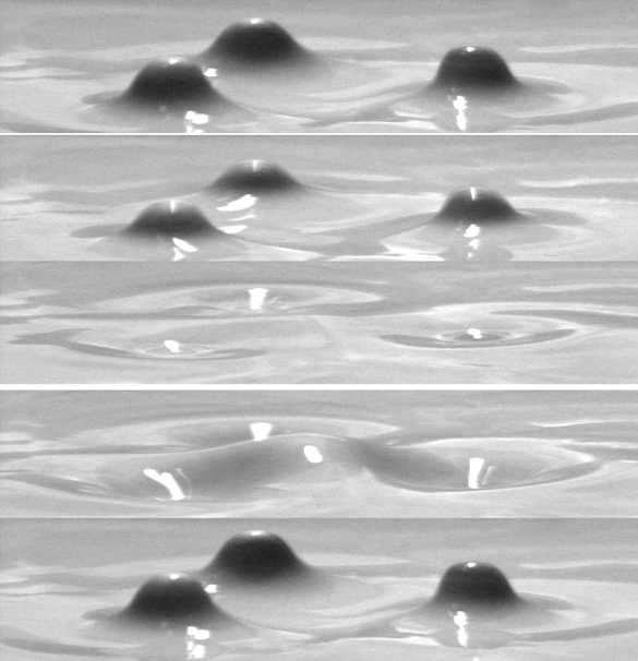
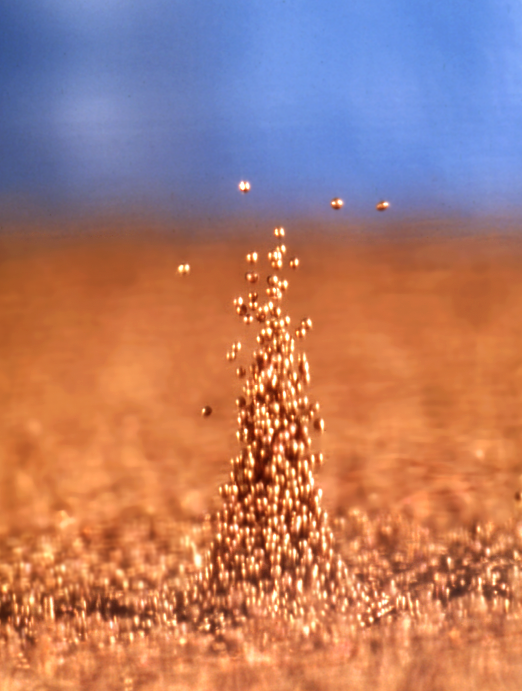
Figure 1: Left: A triad of oscillons in a vertically vibrated colloidal suspension, with time running from top to bottom (taken from [25]). Right: An oscillon in a vertically vibrated layer of bronze beads (courtesy of Paul Umbanhowar, Northwestern University).

A subharmonic standing wave modulated slowly in time is described by an ansatz of the form

(1) $$U(t,x)=A(T)e^{i\Omega t}\cos(kx)+\text{c.c.},$$

for a real scalar variable $U$ depending on a (fast) time variable $t$ and a spatial variable $x$. Here, $A$ is a complex amplitude depending on a slow time scale $T$; also, $k$ is the wavenumber and c.c. stands for complex conjugate. Phase shifts in $A$ correspond to translations in time. Symmetry considerations then lead to an amplitude equation of the form

(2) $$A_{T}=(\rho+i\nu)A+C|A|^{2}A+i\Gamma\bar{A},$$

where the real parameter $\Gamma$ describes the strength of the forcing. The parameters $\rho$ and $\nu$ are real but $C$ is complex. The last term (with $\bar{A}$) breaks the phase symmetry of $A$ and thus the corresponding time-translation symmetry: the phase of $A$ is not arbitrary becuase the forcing in the original system is time dependent. The factor $i$ in the last term can be removed by applying a phase shift. See [17] for a discussion of this (and related) amplitude equations.

In the case of spatially localized oscillons, we also have to include spatial modulations, so that the amplitude $A$ in Eq. 1 depends not only on $T$ but also on a slow spatial variable $X$. It would seem logical that this ansatz would lead to a diffusion term to Eq. 2, yielding a forced complex Ginzburg–Landau (FCGL) equation which is typically written down without derivation [16, 28, 30, 41]:

(3) $$A_{T}=(\rho+i\nu)A-2(\alpha+i\beta)A_{XX}+C|A|^{2}A+i\Gamma\bar{A}.$$

Here, $\alpha$ and $\beta$ are real parameters; the factor $-2$ is included for comparison with the results that we will derive in this paper. Burke, Yochelis and Knobloch [10] showed that this equation admits localized solutions. In [2], the FCGL equation was derived from a model PDE in which patterns are formed with zero wavenumber at onset; the agreement between the localized solutions in the model PDE and those in Eq. 3 was excellent.

However, in the Faraday wave experiment, the preferred wavenumber is non-zero at onset [6]. Nevertheless, the FCGL equation has sometimes been used as an amplitude equation for Faraday wave and granular oscillons [4, 16, 37, 42]. In this paper, we argue that this is not appropriate; instead, a system of two coupled forced complex Ginzburg–Landau equations should be used, as was done in [27, 33].

In order to demonstrate explicitly the origin and correctness of the coupled FCGL equations as amplitude equations for oscillons, we use a PDE model with single-frequency time-dependent forcing, introduced in [34] as phenomenological model of the Faraday wave experiment. We simplify the PDE by removing quadratic terms, and by taking the parametric forcing to be $\cos(2t)$, where $t$ is the fast time scale. The resulting model PDE is then

(4) $$U_{t}=(\mu+i\omega)U+(\alpha+i\beta)U_{xx}+(\gamma+i\delta)U_{xxxx}+C|U|^{2}U+i\operatorname{Re}{(U)}F\cos(2t),$$

where $U(x,t)$ is a complex function, $\mu<0$ is the distance from onset of the oscillatory instability, $\omega$, $\alpha$, $\beta$, $\gamma$, $\delta$ and $F$ are real parameters, and $C$ is a complex parameter. The $\cos(2t)$ term makes this PDE non-autonomous. In this model, the dispersion relation can be readily controlled so the wavenumber at onset can be chosen be zero or non-zero, and the nonlinear terms are chosen to be simple in order that the weakly nonlinear theory and numerical solutions can be computed easily. In [2], the wavenumber at the onset of pattern formation was zero, and the FCGL equation was derived as a description of the localized solution. There, we did not require the fourth-order derivatives in Eq. 4. In contrast, in the current study we use the dispersion relation to set the wavenumber to be 1 at onset, and therefore we need to retain the term $(\gamma+i\delta)U_{xxxx}$ with the fourth-order spatial derivatives.

Our aim is to find and analyze spatially localized oscillons with non-zero wavenumber in the PDE model Eq. 4 theoretically and numerically in 1D and numerically in 2D. The approach will be similar to that in [2], though conceptionally more complicated since we have to consider the interaction between left- and right-travelling waves and the effect of a non-zero group velocity, leading to coupled amplitude equations. Although we will work with a model PDE, our approach will show how localized solutions might be studied in PDEs more directly connected to the Faraday wave experiment, such as the Zhang–Viñals model [43], and how weakly nonlinear calculations from the Navier–Stokes equations [36] might be extended to the oscillons observed in the Faraday wave experiment.

In this case we can model waves with a slowly varying envelope in one spatial dimension by looking at solutions of the form

(5) $$U(x,t)=A(X,T)e^{i(t+x)}+B(X,T)e^{i(t-x)},$$

where $X$ and $T$ are slow scales, and $x$ and $t$ are scaled so that the wave has critical wavenumber $k_{c}=1$ and critical frequency $\Omega_{c}=1$. Commonly the complex conjugate is added to an ansatz of the form Eq. 5 in order to make $U$ real, but our PDE Eq. 4 admits complex solutions (we argue in the conclusion that this does not make a material difference). In order to cover the symmetries of the PDE model, we include both the left- and right-travelling waves (with amplitudes $A$ and $B$, respectively) but the time dependence will be $e^{it}$ only, without $e^{-it}$. In Section 3.1, we explain in detail how the solution of the linear operator, which we will define later, involves $e^{it}$ only. The $+1$ frequency dominates at leading order because of our choice of dispersion relation. Here, we will focus primarily on the one-dimensional case. Two-dimensional localized oscillons are discussed briefly at the end and studied numerically in more detail in [1].

We start by showing some numerical examples of oscillons in the model PDE Eq. 4 and bifurcation diagrams exhibiting snaking, where branches of solutions go back and forth as parameters are varied and the width of the localized pattern increases. We will do an asymptotic reduction of the model PDE to the coupled FCGL equations in the limit of weak damping, weak detuning, weak forcing, small group velocity, and small amplitude, and we will study the properties of the coupled FCGL equations. Some numerical examples of spatially localized oscillons in the coupled FCGL equations will be given. We will also investigate the effect of changing the group velocity. Furthermore, we will reduce the coupled FCGL equations to the real Ginzburg–Landau equation in a further limit of weak forcing and small amplitude close to onset. The real Ginzburg–Landau equation has exact localized sech solutions. Throughout, we will use weakly nonlinear theory by introducing a multiple scale expansion to do the reduction to the amplitude equations. We conclude with numerical examples of strongly localized oscillons in 1D and 2D.

2 Numerical results for the model PDE

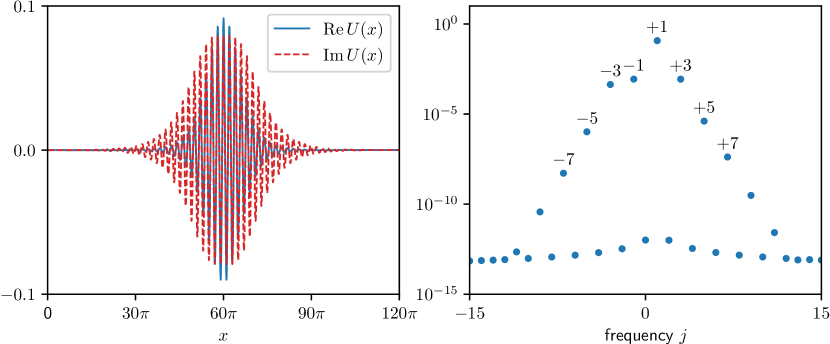
Figure 2: Left: Stable oscillon solution of Eq. 4 found by time-stepping, with $\mu=-0.255$, $\omega=1.5325$, $\alpha=-0.5$, $\beta=1$, $\gamma=-0.25$, $\delta=0.4875$, $C=-1-2.5i$, and $F=0.0585$. The solution is plotted at $t=0$. Right: Amplitude of the $e^{ijt}$ mode with frequency $j$ when expanding the solution in the left panel at $x=60\pi$ as a Fourier series in time: the frequency $+1$ component is the strongest, followed by frequencies $-3$, $-1$ and $+3$, as expected, with the other frequencies at least two orders of magnitude weaker.

Similar to the methodology that was used in [2], we present numerical simulations of the PDE model Eq. 4 by time-stepping and continuation. The choice of parameters is guided by the asymptotic analysis in the remainder of the paper: all modes are damped in the absence of forcing, but the modes with wavenumber $k\simeq\pm 1$ are only weakly damped, the forcing is also weak, and the group velocity is small. We discretize the PDE using a Fourier pseudospectral method and the resulting system of ODEs is solved with a fourth-order exponential time differencing (ETD) method [12]. Most experiments are done on a domain of size $L=120\pi$ (60 wavelengths), in which case we use 2048 grid points. Solving the PDE from an appropriate initial condition, we find the localized solution plotted in the left panel of Fig. 2.

To do continuation from this localized solution, we represent solutions by a truncated Fourier series in time with frequencies $-3$, $-1$, $1$ and $3$. The choice of these frequencies comes from the choice of parameters: the linearized PDE at wavenumber $\pm 1$ looks like $\frac{\partial u}{\partial t}=iu$ (writing $U=u(t)e^{ix}$), so the strongest Fourier component of $u$ looks like $e^{it}$; then putting $u=e^{it}$ into the forcing $\operatorname{Re}(e^{it})\cos(2t)$ generates the frequencies $-3$, $-1$, $1$ and $3$, as described in [2]. We also checked numerically that the frequencies $\pm 1$ and $\pm 3$ dominate (see the right panel of Fig. 2).

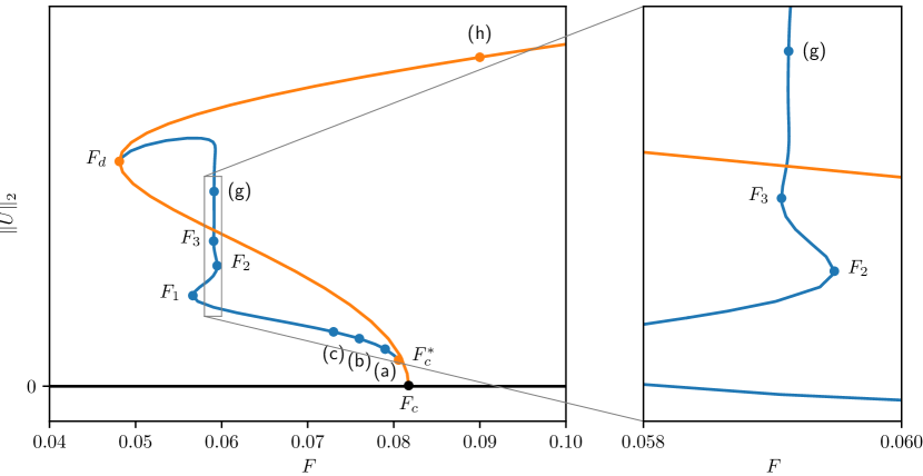
Figure 3: Bifurcation diagram of Eq. 4 in the weak damping limit in a domain of size $L_{x}=120\pi$ with parameters as in Fig. 2. The branch with periodic solutions is plotted in red. The bistability region is between $F_{d}=0.04811$ and $F_{c}=0.08173$. The branch with localized solutions (blue) starts at $F^{*}_{c}=0.08056$ and has folds at $F_{1}=0.05666$, $F_{2}=0.05948$ and $F_{3}=0.05912$. Solutions at (a), (b), (c), $F_{1}$, $F_{2}$, $F_{3}$, (g) and (h) are shown in Fig. 4.

The bifurcation diagram of Eq. 4 as computed by AUTO [18] is given in Fig. 3. The subcritical transition from the zero state to the pattern occurs at the bifurcation point $F_{c}=0.08173$. The saddle-node point where the unstable periodic pattern becomes stable is at $F_{d}=0.04811$. The bistability region where we look for the branch of localized states is between $F_{c}$ and $F_{d}$. The branch of localized solutions bifurcates from the branch of periodic patterns at $F_{c}^{*}=0.08056$, which is away from $F_{c}$ because of the finite domain. Stable localized solutions are located between $F_{1}=0.05666$ and $F_{2}=0.05948$.

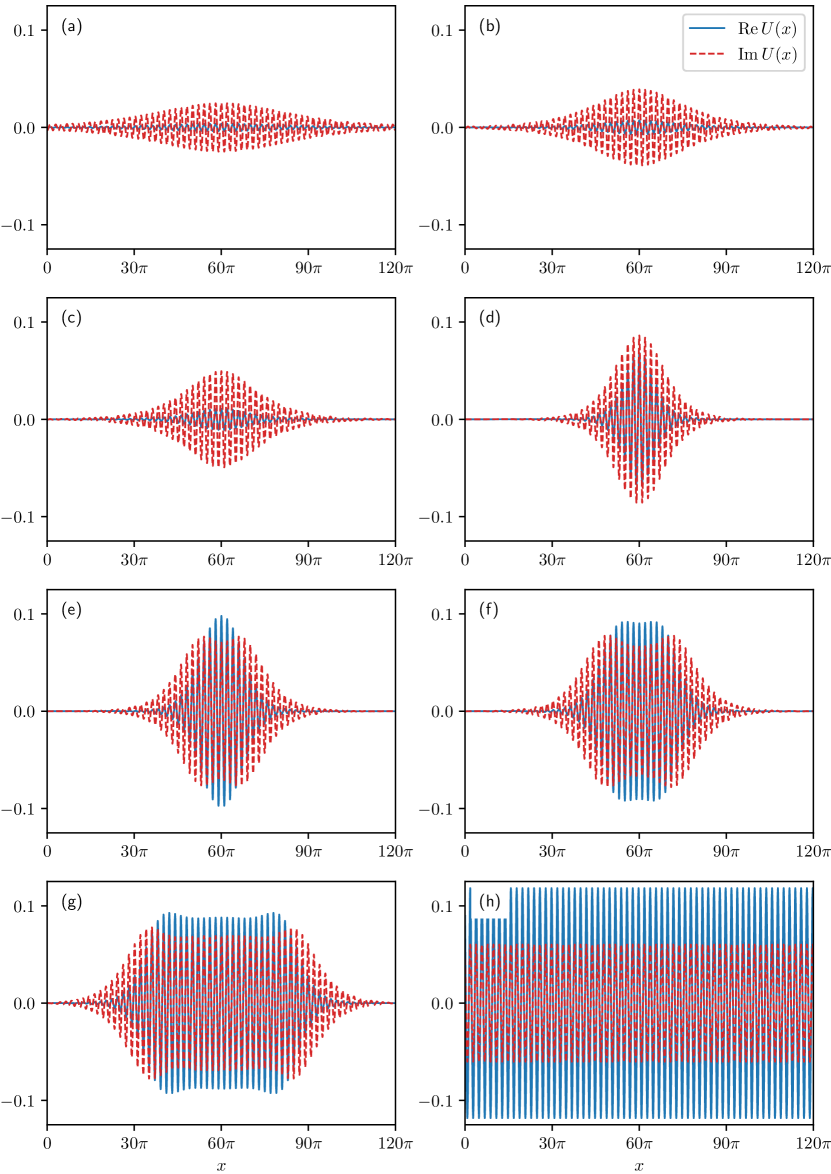
Figure 4: Solutions along the branch of localized solutions in the bifurcation diagram in Fig. 3, at (a) $F=0.079$, (b) $F=0.076$, (c) $F=0.073$, (d) the fold at $F_{1}=0.05666$, (e) the fold at $F_{2}=0.05948$, (f) the fold at $F_{3}=0.05912$, and the point (g). Solution (h) is on the periodic branch at $F=0.09$.

Examples of solutions along the branch of localized solutions in Fig. 3 are given in Fig. 4. Near the point $F_{c}^{*}$ where the branch of localized solutions bifurcates, the localized solutions look like the periodic patterns: small amplitude oscillations which are not very localized (see Fig. 4(a)). As we go along the branch of localized solutions, the amplitude increases and the unstable oscillons become more localized (Fig. 4(b)–(c)). At $F_{1}=0.05695$, the localized oscillons stabilize (Fig. 4(d)) and then they lose stability again at $F_{2}=0.05987$ (Fig. 4(e)) as the branch of solutions snakes back and forth. The next saddle-node point is at $F_{3}=0.05912$ (Fig. 4(f)). It appears from the numerical results that the parameter intervals between successive saddle-node points shrinks to zero as we continue on the branch with localized solutions; this is called collapsed snaking in [28]. However, we suspect that our numerics are misleading, partially because the domain size is too small, and that in fact, the odd and even saddle-node points asymptote to parameter values which are close to each other but not equal. The branch of localized solution connects to the pattern branch close to the saddle-node point $F_{d}$. Figure 4(h) shows a typical periodic pattern. All solutions in Figs. 3 and 4 satisfy $U(x,t)=U(-x,t)$ for a suitably chosen origin. We have not found solutions with any other symmetry.

In the remainder of the paper, we will analyze these oscillons and derive an asymptotic expression for their amplitude, which will be compared to the numerical solutions in Fig. 9.

3 Derivation of the coupled forced complex Ginzburg–Landau (FCGL) equation

In this section we will study the PDE model Eq. 4 in the limit of weak damping, weak detuning, weak forcing and small amplitude in order to derive its amplitude equation. In addition, we will need to assume that the group velocity is small. We start with linearizing Eq. 4 about zero, and we consider solutions of the form $U(x,t)=e^{\sigma t+ikx}$, where $\sigma$ is the complex growth rate of a mode with wavenumber $k$. Without taking any limits and without considering the forcing, the growth rate is given by

(6) $$\sigma=\mu-\alpha k^{2}+\gamma k^{4}+i(\omega-\beta k^{2}+\delta k^{4}),$$

so $\sigma_{r}=\mu-\alpha k^{2}+\gamma k^{4}$ gives the damping rate of modes with wavenumber $k$, and $\sigma_{i}=\omega-\beta k^{2}+\delta k^{4}$ gives the frequency of oscillation. We will also need the group velocity of the waves, which is $d\sigma_{i}(k)/dk=-2\beta k+4\delta k^{3}$.

We will choose parameters so that we are in a weak damping, weak detuning, and small group velocity limit for modes with wavenumber $k=1$. Specifically, in order to find spatially localized oscillons and to do the reduction to the amplitude equation, we will impose the following.

Stability in the absence of forcing

To have waves with all wavenumbers linearly damped, we require that $\sigma_{r}(k)<0$, for all $k$. It follows that $\mu<0$, $\alpha>-2\sqrt{\mu\gamma}$ and $\gamma<0$. With $\alpha<0$ we have a non-monotonic growth rate.

Preferred wavenumber

We want the damping to be weakest for $k=\pm 1$. Thus, we require that the growth rate $\sigma_{r}$ achieves a maximum when the wavenumber $k$ is 1, so $\frac{d}{dk}\sigma_{r}(k=1)=-2\alpha+4\gamma=0$. This gives the condition $\alpha=2\gamma$.

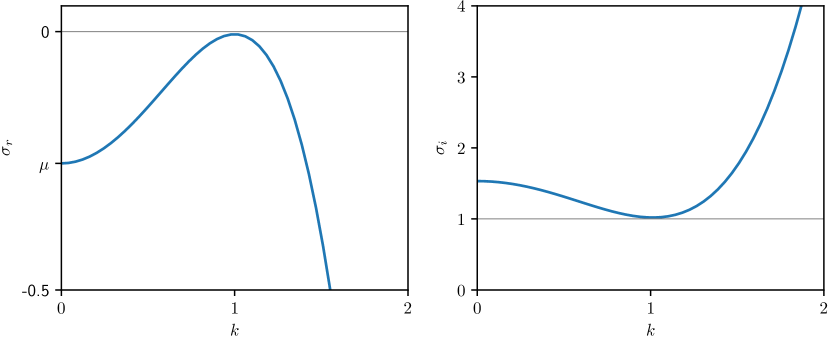
Figure 5: The growth rate (left panel) and dispersion relation (right panel) of equation Eq. 4 with $\mu=-0.255$, $\omega=1.5325$, $\alpha=-0.5$, $\beta=1$, $\gamma=-0.25$ and $\delta=0.4875$. In this case, the group velocity is small at $k=1$ because this is close to the minimum of the dispersion relation.

Weak damping

We also need to make the growth rate $\sigma_{r}$ to be close to zero when $k=\pm 1$. Therefore, we introduce a small parameter $\epsilon\ll 1$ and a new parameter $\rho$, so that we have $\sigma_{r}(k=1)=\mu-\alpha+\gamma=\epsilon^{2}\rho$, where $\rho<0$. Thus, $\mu=\frac{1}{2}\alpha+\epsilon^{2}\rho$. Figure 5(a) shows an example of the real part of the growth rate.

Weak detuning

We want waves with $k\simeq\pm 1$ to be subharmonically driven by $\cos(2t)$, so the frequency of the oscillation $\sigma_{i}$ should be close to $1$ at $k=1$. Therefore, we write $\sigma_{i}(k=1)=\omega-\beta+\delta=1+\epsilon^{2}\nu$, where $\nu$ is the detuning.

Small group velocity

We require the group velocity $\frac{d\sigma_{i}}{dk}=-2k\beta+4\delta k^{3}$ to be $O(\epsilon)$ at $k=\pm 1$, so we have $-2\beta+4\delta=\epsilon v_{g}$. This is needed to allow the group velocity in the subsequent amplitude equations to appear at the same order as all the other terms. We discuss the consequences of choosing a small group velocity in Section 6. Figure 5(b) shows an example of the dispersion relation $\sigma_{i}(k)$.

Weak forcing

To perform the weakly nonlinear theory, we assume that the forcing is weak, and so we scale the forcing amplitude to be $O(\epsilon^{2})$, writing $F=4\epsilon^{2}\Gamma$.

Table 1: Relationships between parameters $(\mu,\omega,\alpha,\beta,\gamma,\delta,F)$ of the PDE model and the parameters $(\rho,\nu,\alpha,\beta,v_{g},\Gamma)$ of the coupled FCGL equations. Note that these relationships depend on the choice of $\epsilon$. The parameters $\alpha$ and $\beta$ are the same in both models.

The PDE model Eq. 4	The coupled FCGL Eq. 14	Physical meaning
$\mu=\alpha-\gamma+\epsilon^{2}\rho=\frac{1}{2}\alpha+\epsilon^{2}\rho$	$\rho=\dfrac{\mu-\alpha+\gamma}{\epsilon^{2}}$	$\rho=\text{damping ($\rho<0$)}$
$\gamma=\frac{1}{2}\alpha$
$\delta=\frac{1}{2}\beta+\frac{1}{4}\epsilon v_{g}$	$v_{g}=\dfrac{-2\beta+4\delta}{\epsilon}$	$v_{g}=\text{group velocity}$
$\omega=1+\frac{1}{2}\beta-\frac{1}{4}\epsilon v_{g}+\epsilon^{2}\nu$	$\nu=\dfrac{\omega-1-\beta+\delta}{\epsilon^{2}}$	$\nu=\text{detuning}$
$F=4\epsilon^{2}\Gamma$	$\Gamma=\dfrac{F}{4\epsilon^{2}}$	$\Gamma={}$ strength of parametric forcing

We relate the parameters in the PDE model with the parameters in the amplitude equations in a way that we can connect examples of localized oscillons in both equations. In Table 1 all PDE parameters are defined in terms of parameters that will appear in the coupled FCGL equations, and vice versa.

3.1 Linear theory

With the parameters as in Table 1, the linear theory of the PDE Eq. 4 at leading order is given by

(7) $$U_{t}=\left(\frac{\alpha}{2}+i\left(\frac{\beta}{2}+1\right)\right)U+\left(\alpha+i\beta\right)U_{xx}+\left(\frac{\alpha}{2}+i\frac{\beta}{2}\right)U_{xxxx},$$

which defines a linear operator $L$ as

$$LU=\left(-\frac{\partial}{\partial t}+i\right)U+\left(\frac{\alpha}{2}+i\frac{\beta}{2}\right)\left(1+\frac{\partial^{2}}{\partial x^{2}}\right)^{2}U.$$

This is essentially the linear part of the complex Swift–Hohenberg equation [3], which has appeared in the context of nonlinear optics [23] and Taylor–Couette flows [7]. To find all solutions, we substitute $U=e^{\sigma t+ikx}$ into the above equation to get the dispersion relation

$$\sigma=i+\left(\frac{\alpha}{2}+i\frac{\beta}{2}\right)\left(1-k^{2}\right)^{2}.$$

We assume that our problem has periodic boundary conditions, which implies that $k\in\mathbb{R}$. Furthermore, we require $\sigma_{r}=0$ since we are considering neutral modes. The real and imaginary parts of this equation give

$$k=\pm 1\quad\text{and}\quad\sigma=i.$$

Therefore, $LU=0$, equivalent to Eq. 7, implies that neutral modes are a linear combinations of $U(x,t)=e^{i(t+x)}$ and $U(x,t)=e^{i(t-x)}$. Note that our choice of dispersion relation leads to positive frequency solutions. This is not a severe restriction, as discussed in Section 6.

3.2 Weakly nonlinear theory

In order to apply the standard weakly nonlinear theory, we need the adjoint linear operator $L^{\dagger}$. Therefore, we define an inner product between two functions $f(x,t)$ and $g(x,t)$ by

(8) $$\big{\langle}f(x,t),g(x,t)\big{\rangle}=\frac{1}{4\pi^{2}}\int_{0}^{2\pi}\int_{0}^{2\pi}\bar{f}(x,t)g(x,t)\,dt\,dx,$$

where $\bar{f}$ is the complex conjugate of $f$. The adjoint linear operator $L^{\dagger}$ is defined by the relation

$$\big{\langle}f(x,t),Lg(x,t)\big{\rangle}=\big{\langle}L^{\dagger}f(x,t),g(x,t)\big{\rangle}\qquad\text{for all $f$ and $g$},$$

and so, using integration by parts,

$$L^{\dagger}f=\left(\frac{\partial}{\partial t}-i+\left(\frac{\alpha}{2}-i\frac{\beta}{2}\right)\left(1+\frac{\partial^{2}}{\partial x^{2}}\right)^{2}\right)f.$$

Taking the adjoint changes the sign of the $\frac{\partial}{\partial t}$ term and takes the complex conjugate of other terms of $L$. The adjoint eigenfunctions are then given by solving $L^{\dagger}f=0$; the solutions are also linear combinations of $e^{i(t\pm x)}.$

We expand $U$ in powers of the small parameter $\epsilon$:

(9) $$U=\epsilon U_{1}+\epsilon^{2}U_{2}+\epsilon^{3}U_{3}+\cdots,$$

where $U_{1}$, $U_{2}$, $U_{3}$, …are $O(1)$ complex functions. We will derive solutions $U_{1}$, $U_{2}$, $U_{3}$, …at each order of $\epsilon$.

At $O(\epsilon)$, the linear theory arises and we find $LU_{1}=0$. The solution $U_{1}$ takes the form

(10) $$U_{1}=A(X,T)e^{i(t+x)}+B(X,T)e^{i(t-x)},$$

where $A$ and $B$ represent the amplitudes of the left and right travelling waves. They are functions of $X$ and $T$, the long and slow scale modulations of space and time variables:

$$T=\epsilon^{2}t,\quad{}\text{and}\quad{}X=\epsilon x.$$

The multiple scale expansion below will determine the evolution equations for $A(X,T)$ and $B(X,T)$.

At second order in $\epsilon$, we get $LU_{2}=0$: the $\frac{\partial^{2}U_{1}}{\partial x\partial X}$ term cancels with the $\frac{\partial^{4}U_{1}}{\partial x^{3}\partial X}$ term. We would have had a forcing term at this order if we had not ensured that the group velocity is $O(\epsilon)$. The equation at this order is solved by setting $U_{2}=0$.

At third order in $\epsilon$, we get

(11) $$\frac{\partial U_{1}}{\partial T} =LU_{3}+(\rho+i\nu)U_{1}+(\alpha+i\beta)\frac{\partial^{2}U_{1}}{\partial X^{2}}+3(\alpha+i\beta)\frac{\partial^{4}U_{1}}{\partial x^{2}\partial X^{2}}$$

$$\quad{}+iv_{g}\frac{\partial^{4}U_{1}}{\partial x^{3}\partial X}+4i\Gamma\cos(2t)\operatorname{Re}(U_{1})+C|U_{1}|^{2}U_{1}.$$

The linear operator $L$ is singular so we must apply a solvability condition: we take the inner product between the adjoint eigenfunction $e^{i(t+x)}$ and equation Eq. 11, which gives

(12) $$\left\langle e^{i(t+x)},\frac{\partial U_{1}}{\partial T}\right\rangle =\left\langle e^{i(t+x)},LU_{3}\right\rangle+(\rho+i\nu)\left\langle e^{i(t+x)},U_{1}\right\rangle+(\alpha+i\beta)\left\langle e^{i(t+x)},\frac{\partial^{2}U_{1}}{\partial X^{2}}\right\rangle$$

$$\quad{}+3(\alpha+i\beta)\left\langle e^{i(t+x)},\frac{\partial^{4}U_{1}}{\partial x^{2}\partial X^{2}}\right\rangle+iv_{g}\left\langle e^{i(t+x)},\frac{\partial^{4}U_{1}}{\partial x^{3}\partial X}\right\rangle$$

$$\quad{}+4i\Gamma\left\langle e^{i(t+x)},\cos(2t)\operatorname{Re}(U_{1})\right\rangle+C\left\langle e^{i(t+x)},|U_{1}|^{2}U_{1}\right\rangle.$$

We have $\langle e^{i(t+x)},LU_{3}\rangle=\langle L^{\dagger}e^{i(t+x)},U_{3}\rangle=0$, so $U_{3}$ is removed and the above equation becomes an equation in $U_{1}$ only. Substituting the solution $U_{1}$ leads to

(13) $$\left\langle e^{i(t+x)},\frac{\partial}{\partial T}(Ae^{i(t+x)}+Be^{i(t-x)})\right\rangle$$

$$=(\rho+i\nu)\left\langle e^{i(t+x)},Ae^{i(t+x)}+Be^{i(t-x)}\right\rangle$$

$$\qquad{}+(\alpha+i\beta)\left\langle e^{i(t+x)},\frac{\partial^{2}}{\partial X^{2}}(Ae^{i(t+x)}+Be^{i(t-x)})\right\rangle$$

$$\qquad{}+3(\alpha+i\beta)\left\langle e^{i(t+x)},\frac{\partial^{4}}{\partial x^{2}\partial X^{2}}(Ae^{i(t+x)}+Be^{i(t-x)})\right\rangle$$

$$\qquad{}+iv_{g}\left\langle e^{i(t+x)},\frac{\partial^{4}}{\partial x^{3}\partial X}(Ae^{i(t+x)}+Be^{i(t-x)})\right\rangle$$

$$\qquad{}+4i\Gamma\left\langle e^{i(t+x)},\tfrac{1}{2}\cos(2t)(Ae^{i(x+t)}+Be^{i(t-x)}+\bar{A}e^{-i(t+x)}+\bar{B}e^{-i(t-x)})\right\rangle$$

$$\qquad{}+C\left\langle e^{i(t+x)},(|A|^{2}+A\bar{B}e^{2ix}+\bar{A}Be^{-2ix}+|B|^{2})(Ae^{i(t+x)}+Be^{i(t-x)})\right\rangle.$$

After we compute the left and right hand sides of the above equation term by term, we get equations for the amplitudes $A(X,T)$ and $B(X,T)$:

(14) $$\frac{\partial A}{\partial T} =(\rho+i\nu)A-2(\alpha+i\beta)\frac{\partial^{2}A}{\partial X^{2}}+v_{g}\frac{\partial A}{\partial X}+C(|A|^{2}+2|B|^{2})A+i\Gamma\bar{B},$$

$$\frac{\partial B}{\partial T} =(\rho+i\nu)B-2(\alpha+i\beta)\frac{\partial^{2}B}{\partial X^{2}}-v_{g}\frac{\partial B}{\partial X}+C(2|A|^{2}+|B|^{2})B+i\Gamma\bar{A}.$$

Thus the PDE model has been reduced to the coupled FCGL equations in the weak damping, weak detuning, small group velocity and small amplitude limit. In equations Eq. 14 the group velocity terms have different signs, which makes the envelopes travel in opposite directions. The $-2\alpha\frac{\partial^{2}A}{\partial X^{2}}$ may make the above equations look like they are ill posed, but recall that $\alpha<0$.

4 Properties of the coupled FCGL equations

Following [21] we can identify the symmetries and how they affect the structure of Eq. 14. The original system is invariant under translations in $x$: Replacing $x$ by $x+\phi^{*}$, where $\phi^{*}$ is arbitrary, we get

$$U(x+\phi^{*},t)=A(X+\epsilon\phi^{*},T)\,e^{i(t+x+\phi^{*})}+B(X+\epsilon\phi^{*},T)\,e^{i(t-x-\phi^{*})},$$

which is also a solution of the problem. This translation has the effect of shifting $X$ to $X+\epsilon\phi^{*}$, and changing the phase of $A$ and $B$: If we suppress the change from $X$ to $X+\epsilon\phi^{*}$, then Eq. 14 is equivariant under

$$A\rightarrow Ae^{i\phi^{*}},\quad B\rightarrow Be^{-i\phi^{*}},$$

which is therefore a symmetry of Eq. 14. Equations Eq. 14 are also invariant under translations in $X$, but this is an artifact of the truncation at cubic order [29]. Similarly, we can reflect in $x$, which leads to the symmetry $A\leftrightarrow B$, $\partial_{x}\leftrightarrow-\partial_{x}$.

Amplitude equations associated with a Hopf bifurcation (a weakly damped Hopf bifurcation in this case) usually have time translation symmetry, which manifests as equivariance under phase shifts of the amplitudes. However, the underlying PDE is non-autonomous, and so rotating $A$ and $B$ by a common phase is not a symmetry of Eq. 14. Equations Eq. 14 do posess $T$-translation symmetry, but this is also an artifact.

The parametric forcing provides an interesting coupling between the left and right travelling waves with amplitudes $A$ and $B$, which means that solutions or symmetries that one might expect at first glance, are in fact not present. For example, the coupling terms in the coupled FCGL equations make it impossible to find pure travelling waves; i.e., $A\neq 0$, $B=0$ is not a solution of Eq. 14. Also, solutions with $A=B$ exist only if $v_{g}$ is zero, which generically it is not. Finally, steady standing wave solutions (which are typically seen in Faraday wave experiments) have $B(X)=A(-X)$; substituting this into Eq. 14 yields a nonlocal equation that is not a PDE, though all solutions we present in this paper are in this category.

4.1 The zero solution

The stability of the zero state under small perturbations with complex growth rate $s$ and real wavenumber $q$ can be studied by linearizing Eq. 14, writing $A$ and $B$ as

$$A=\hat{A}e^{sT+iqX},\quad\text{and}\quad B=\hat{B}e^{\bar{s}T-iqX},$$

where $|\hat{A}|\ll 1$, $|\hat{B}|\ll 1$ and $\hat{A},\hat{B}\in\mathbb{C}$. We choose $\hat{B}e^{\bar{s}T-iqX}$ in order that the exponential term will cancel in the next step. Substituting this into equation Eq. 14, linearizing and taking the complex conjugate of the second equation gives:

(15) $$s\hat{A} =(\rho+i\nu)\hat{A}+2(\alpha+i\beta)q^{2}\hat{A}+iv_{g}q\hat{A}+i\Gamma\bar{\hat{B}}.$$

$$s\bar{\hat{B}} =(\rho-i\nu)\bar{\hat{B}}+2(\alpha-i\beta)q^{2}\bar{\hat{B}}-iv_{g}q\bar{\hat{B}}-i\Gamma\hat{A}.$$

This is a linear homogeneous system of equations, so there is a nontrivial solution only when its determinant is zero. The imaginary part of the determinant equals $2s_{i}(\rho+2\alpha q^{2}-s_{r})$, where $s_{r}$ and $s_{i}$ denote the real and imaginary part of $s$. We are interested in locating the bifurcation where zero solution is neutrally stable, so $s_{r}=0$. Since $\rho$ and $\alpha$ are negative, the determinant can only be zero if $s_{i}=0$. Thus, there is no Hopf bifurcation, and the neutral stability condition is $s=0$. Setting the real part of the determinant of Eq. 15 equal to zero leads to:

(16) $$(\rho+2\alpha q^{2})^{2}+(\nu+2\beta q^{2}+v_{g}q)^{2}=\Gamma^{2}.$$

The stability of the zero state changes when $\Gamma=\Gamma_{c}$, the minimum of the neutral stability curve, and the non-zero flat state is created with $q=q_{c}$. This corresponds to a uniform pattern in the PDE Eq. 4 with wavenumber $k_{c}=1+\epsilon q_{c}$. The critical wavenumber $q_{c}$ can be computed by minimizing the left-hand side of equation Eq. 16. Differentiating with respect to $q$ yields the following cubic equation in $q$:

(17) $$4\alpha q(\rho+2\alpha q^{2})+(4\beta q+v_{g})(\nu+2\beta q^{2}+v_{g}q)=0.$$

Solving this gives $q_{c}$, the critical wavenumber, which is positive if $\nu v_{g}<0$ and negative if $\nu v_{g}>0$. Substituting $q=q_{c}$ into Eq. 16 gives $\Gamma_{c}$.

4.2 Standing waves

Now we look at steady equal-amplitude states of the form $A=R_{0}e^{i(qX+\phi_{1})}$ and $B=R_{0}e^{i(-qX+\phi_{2})}$, where $R_{0}$ and $q$ are real, and $\phi_{1}$ and $\phi_{2}$ are the phases. These represent uniform standing wave patterns with wavenumber $1+\epsilon q$ in $U(x)$. We substitute this into equations Eq. 14, which yields, assuming that $R_{0}$ is not zero,

$$0=(\rho+i\nu)+2(\alpha+i\beta)q^{2}+iv_{g}q+3CR_{0}^{2}+i\Gamma e^{-i\Phi},$$

where $\Phi=\phi_{1}+\phi_{2}$. This is the same equation obtained for steady constant-amplitude solutions of the single FCGL equation Eq. 3, but with a group velocity term. The real and imaginary parts of the above equation are

(18) $$\text{Re:}\quad 0 =\rho+2\alpha q^{2}+3C_{r}R_{0}^{2}+\Gamma\sin\Phi.$$

$$\text{Im:}\quad 0 =\nu+2\beta q^{2}+v_{g}q+3C_{i}R_{0}^{2}+\Gamma\cos\Phi.$$

We eliminate $\Phi$ by using the identity $\cos^{2}\Phi+\sin^{2}\Phi=1$ to give the following polynomial equation for $R_{0}$:

(19) $$0=9(C_{r}^{2}+C_{i}^{2})R_{0}^{4}+6\left((\rho+2\alpha q^{2})C_{r}+(\nu+v_{g}q+2\beta q^{2})C_{i}\right)R_{0}^{2}\\ +(\rho+2\alpha q^{2})^{2}+(\nu+v_{g}q+2\beta q^{2})^{2}-\Gamma^{2}.$$

This is a quadratic equation in $R_{0}^{2}$ and its discriminant is given by

$$\Delta=36\left((\rho+2\alpha q^{2})C_{r}+(\nu+v_{g}q+2\beta q^{2})C_{i}\right)^{2}\\ -36\left((\rho+2\alpha q^{2})^{2}+(\nu+v_{g}q+2\beta q^{2})^{2}-\Gamma^{2}\right)(C_{r}^{2}+C_{i}^{2}).$$

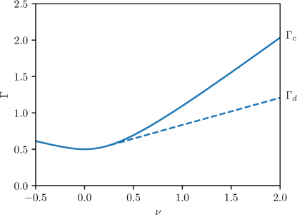
Figure 6: The $(\nu,\Gamma)$ parameter plane of the coupled FCGL equations Eq. 14 with $\rho=-0.5$, $\alpha=-0.5$, $\beta=1$, $v_{g}=-0.5$ and $C=-1-2.5i$. These parameters with $\epsilon=0.1$ correspond to the prameters of the model PDE Eq. 4 used in the figures in Section 2. The solid line shows the primary pitchfork bifurcation at $\Gamma_{c}$, where the zero state becomes unstable to perturbations with wavenumber $q_{c}$. The dash line shows the saddle-node bifurcation at $\Gamma_{d}$.

Examination of the polynomial Eq. 19 shows that when the forcing amplitude $\Gamma$ reaches $((\rho+2\alpha q^{2})^{2}+(\nu+v_{g}q+2\beta q^{2})^{2})^{1/2}$, a subcritical bifurcation occurs provided that $(\rho+2\alpha q^{2})C_{r}+(\nu+v_{g}q+2\beta q^{2})C_{i}<0$. Spatially oscillatory states $A^{-}_{sp}$ and $B^{-}_{sp}$ are created, which turn into $A^{+}_{sp}$ and $B^{+}_{sp}$ states at a saddle-node ($\Delta=0$) bifurcation at $\Gamma=\Gamma_{d}$, with

(20) $$\Gamma_{d}=\sqrt{(\rho+2\alpha q^{2})^{2}+(\nu+v_{g}q+2\beta q^{2})^{2}-\frac{((\rho+2\alpha q^{2})C_{r}+(\nu+v_{g}q+2\beta q^{2})C_{i})^{2}}{C_{r}^{2}+C_{i}^{2}}}.$$

Figure 6 shows equations Eq. 16 and Eq. 20 in the $(\nu,\Gamma)$ parameter plane where we have taken $q=q_{c}$ from Eq. 17. The values of the parameters $\rho$, $\alpha$, $\beta$, $v_{g}$, $C_{r}$ and $C_{i}$ in the figure correspond to the parameters in the figures in Section 2 with $\epsilon=0.1$. The primary bifurcation changes from supercritical to subcritical when $(\rho+2\alpha q^{2})C_{r}+(\nu+v_{g}q+2\beta q^{2})C_{i}=0$, which is at $\nu=0.2228$ for the parameter values in Fig. 6. Localized solutions can be found in the bistability region between $\Gamma_{c}$ and $\Gamma_{d}$.

4.3 Localized solutions

In order to find localized solutions of the coupled FCGL equations Eq. 14, one might attempt an ansatz of the form

$$A=R_{0}(X,T)\,e^{i(qX+\phi_{1})}\quad\text{and}\quad B=\bar{R}_{0}(X,T)\,e^{i(-qX+\phi_{2})}$$

with $R_{0}$ complex and $q,\phi_{1},\phi_{2}$ real. This is a spatially modulated version of the standing wave studied in the previous section. However, the coupled FCGL equations admit no solution of this form, even if $v_{g}=0$. Other standing wave ansatzes are possible, e.g. $A=R_{0}(X)\,e^{i(qX+\phi_{1})}$ and $B=\bar{R}_{0}(-X)\,e^{i(-qX+\phi_{2})}$, but we have not explored these further.

We were able to find analytic expressions for localized solutions of the coupled FCGL equations by taking further asymptotic limits (see Section 5). To motivate the subsequent calculations, we present some numerical examples of stable spatially localized oscillons in the coupled FCGL equations found by using the same numerical method as in Section 2 on a periodic domain of size $20\pi$. We take the same parameter values as before: $\rho=-0.5,$ $\nu=2$, $\alpha=-0.5$, $\beta=1$, and $C=-1-2.5i$.

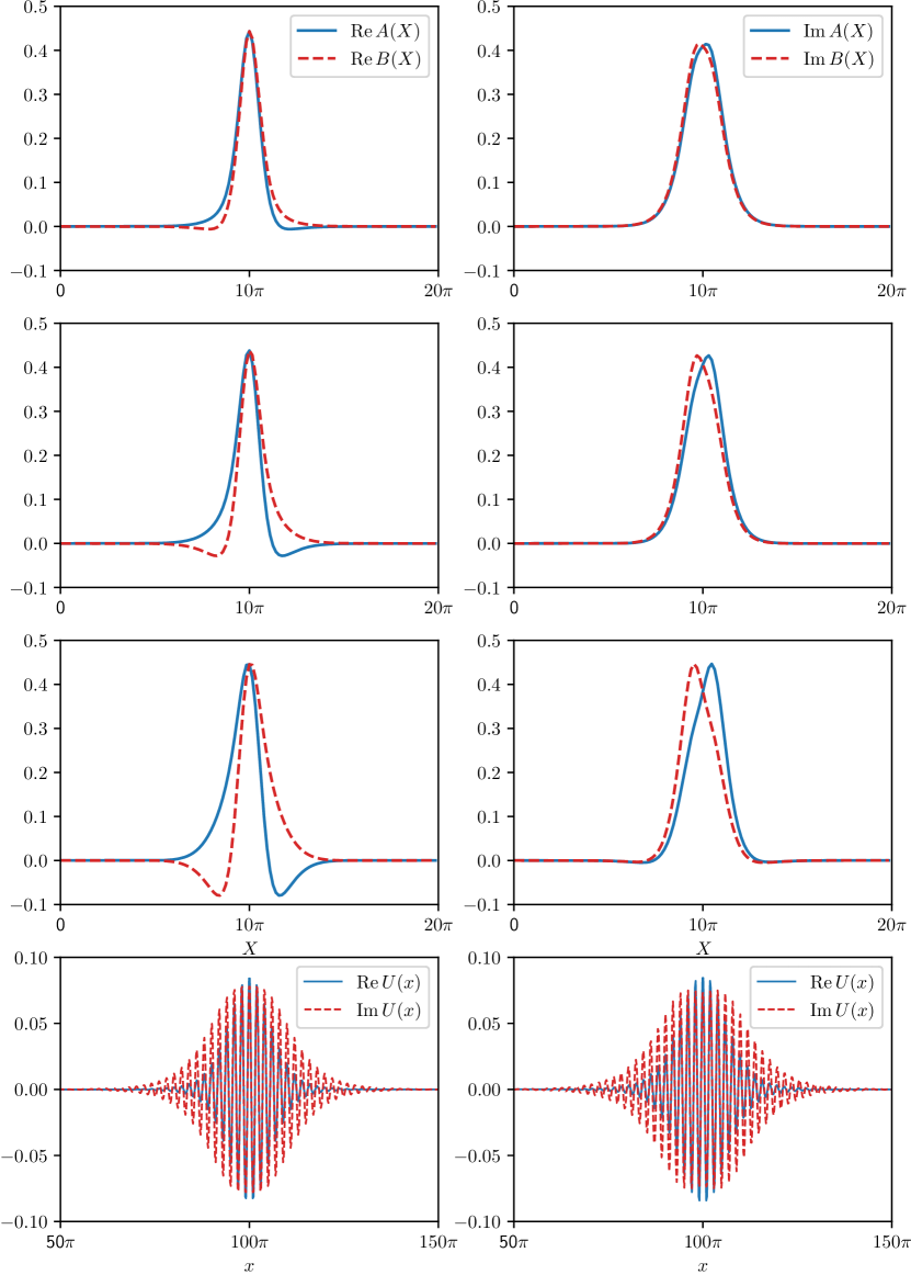
Figure 7: Stationary solutions to the coupled FCGL equations Eq. 14 with $\rho=-0.5$, $\nu=2$, $\alpha=-0.5$, $\beta=1$ and $C=-1-2.5i$. Top row: $v_{g}=-0.2$ and $\Gamma=1.46$. Second row: $v_{g}=-0.5$ and $\Gamma=1.45$. Third row: $v_{g}=-1$ and $\Gamma=1.43$. Bottom row: Approximate solutions $U(x)$ of the PDE model Eq. 4 reconstructed from the solutions $A(X),B(X)$ to the coupled FCGL equations assuming $\epsilon=0.1$; the left and right plots correspond to the top and third rows, respectively.

The top row of Fig. 7 shows an example of a localized oscillon in the coupled FCGL equations with $v_{g}=-0.2$. As we increase the magnitude of the group velocity $v_{g}$ to $v_{g}=-0.5$ (second row) and $v_{g}=-1$ (third row) and change the forcing strength $\Gamma$ so that we are still in the region where the localized solution is stable, we can see that $A$ and $B$ start to move apart, pulled in opposite directions by the group velocity term. We can use these solutions to the coupled FCGL equations to reconstruct first-order approximations to solutions of the PDE model Eq. 4 with the help of Eqs. 9 and 10; this is shown in the bottom row of Fig. 7.

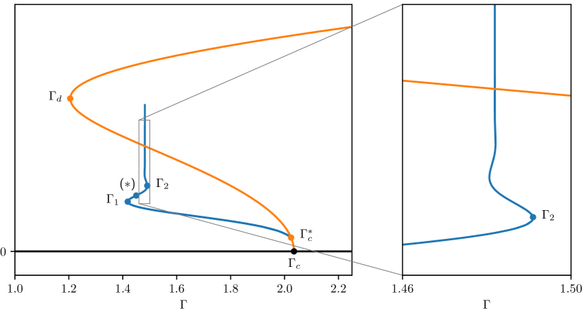
Figure 8: Bifurcation diagram of the coupled FCGL equations with parameters $\rho=-0.5$, $\nu=2$, $\alpha=-0.5$, $\beta=1$, $C=-1-2.5i$ and $v_{g}=-0.5$ (corresponding to Fig. 3). The bifurcations are at $\Gamma_{c}=2.035$, $\Gamma_{d}=1.206$, $\Gamma_{c}^{*}=2.024$, $\Gamma_{1}=1.418$ and $\Gamma_{2}=1.491$. The solution marked ($*$) is shown in the middle row of Fig. 7. Numerical results with AUTO suggest that snaking continues beyond $\Gamma_{2}$, but it is too small to see.

We also computed the bifurcation diagram of the coupled FCGL equations on a domain of size $20\pi$ using AUTO [18]. The critical wavenumber with the above parameter values is $q_{c}=0.09950\approx\frac{1}{10}$, so the periodic solution fits almost perfectly in this domain. The result is shown in Fig. 8. The branch of periodic solution bifurcates from the zero solution at $\Gamma_{c}=2.035$ and has a fold at $\Gamma_{d}=1.206$. Using the relation $F=4\epsilon^{2}\Gamma$, we can compute the corresponding values of forcing in the model PDE Eq. 4 as $0.08140$ and $0.04820$, which agree well with the values of $F_{c}=0.08173$ and $F_{d}=0.04811$ found in Fig. 3 when we applied AUTO directly to the model PDE.

Going back to the coupled FCGL equations, we see a secondary bifurcation at $\Gamma=2.024$ where a branch of localized solutions bifurcates from the branch of periodic solutions. The localized branch has folds at $\Gamma_{1}=1.418$ and $\Gamma_{2}=1.491$. The corresponding $F$ values in terms of the parameters of the model PDE are $0.05673$ and $0.05964$, which again agree well with the values of $F_{1}=0.05666$ and $F_{2}=0.05948$ found in Fig. 3.

As shown in Fig. 8, the localized branch in the bifurcation diagram of the coupled FCGL equations continues to snake upwards after $\Gamma_{2}$. We believe that these exhibit collapsed snaking, where the saddle node points asymptote to one value of $\Gamma$ as one goes up the branch [28]. However, the bifurcation diagram shows that the branch of localized solutions suddenly stops. In fact, AUTO turns around at that point. We believe that this may be caused by AUTO having difficulty handling the phase symmetry in the coupled FCGL equations, and that in reality the branch of localized solutions joins with the branch of periodic solutions near the fold at $\Gamma_{d}$, as it does in the bifurcation diagram of the model PDE in Fig. 3.

5 Reduction to the real Ginzburg–Landau equation

In this section we will reduce the coupled FCGL equations to the real Ginzburg–Landau equation close to the subcritical bifurcation from the zero solution to the constant amplitude state. The reduction was done by Riecke [33] in the supercritical case.

We take the complex conjugate of the second equation of Eq. 14, so the coupled FCGL equations become

(21) $$\frac{\partial A}{\partial T} =D_{1}A+D_{2}\frac{\partial^{2}A}{\partial X^{2}}+v_{g}\frac{\partial A}{\partial X}+C(|A|^{2}+2|B|^{2})A+i\Gamma\bar{B},$$

$$\frac{\partial\bar{B}}{\partial T} =\bar{D}_{1}\bar{B}+\bar{D}_{2}\frac{\partial\bar{B}}{\partial X^{2}}-v_{g}\frac{\partial\bar{B}}{\partial X}+\bar{C}(2|A|^{2}+|B|^{2})\bar{B}-i\Gamma A.$$

For simplicity, we write

(22) $$D_{1}=\rho+i\nu\quad\text{and}\quad D_{2}=-2(\alpha+i\beta).$$

In order to reduce the coupled FCGL equation to the real Ginzburg–Landau equation, we apply weakly nonlinear theory close to onset, writing

$$\Gamma=\Gamma_{c}(1+\epsilon_{2}^{2}\Gamma_{2}),$$

where $0<\epsilon_{2}\ll 1$, and $\Gamma_{c}$ is the critical forcing at critical wavenumber $q_{c}$, and $\Gamma_{2}$ is the new bifurcation parameter. We expand the solution in powers of the new small parameter $\epsilon_{2}$ as follows

$$\begin{bmatrix}A\\ \bar{B}\end{bmatrix}=\begin{bmatrix}\epsilon_{2}A_{1}+\epsilon_{2}^{2}A_{2}+\epsilon_{2}^{3}A_{3}+\cdots\\ \epsilon_{2}\bar{B}_{1}+\epsilon_{2}^{2}\bar{B}_{2}+\epsilon_{2}^{3}\bar{B}_{3}+\cdots\end{bmatrix}.$$

From Section 4.1, the growth rate is real with frequency zero (locked to the forcing), so we scale

$$\frac{\partial}{\partial T}\rightarrow\epsilon_{2}^{2}\frac{\partial}{\partial\tilde{T}},$$

and the preferred wavenumber $q_{c}\neq 0$, so

$$\frac{\partial}{\partial X}\rightarrow\frac{\partial}{\partial X}+\epsilon_{2}\frac{\partial}{\partial\tilde{X}},$$

where $\tilde{X}$ and $\tilde{T}$ are very long space and slow time scales.

At $O(\epsilon_{2})$, we have

$$0 =D_{1}A_{1}+D_{2}\frac{\partial^{2}A_{1}}{\partial X^{2}}+v_{g}\frac{\partial A_{1}}{\partial X}+i\Gamma_{c}\bar{B}_{1},$$

$$0 =\bar{D}_{1}\bar{B}_{1}+\bar{D}_{2}\frac{\partial\bar{B}_{1}}{\partial X^{2}}-v_{g}\frac{\partial\bar{B}_{1}}{\partial X}-i\Gamma_{c}A_{1}.$$

We can solve the above system by assuming that

(23) $$A_{1}=P(\tilde{X},\tilde{T})e^{iq_{c}X}\quad\text{and}\quad B_{1}=Q(\tilde{X},\tilde{T})e^{-iq_{c}X}.$$

At this order of $\epsilon_{2}$, the coupled FCGL equations become

(24) $$0 =D_{1}P-D_{2}q^{2}_{c}P+iv_{g}q_{c}P+i\Gamma_{c}\bar{Q},$$

$$0 =\bar{D}_{1}\bar{Q}-\bar{D}_{2}q^{2}_{c}\bar{Q}-iv_{g}q_{c}\bar{Q}-i\Gamma_{c}P.$$

These can be solved as in Section 4.1.

Additionally, from the first equation of Eq. 24 we get a phase relation between $P$ and $Q$:

(25) $$\bar{Q}=Pe^{i\phi}\quad\text{where}\quad e^{i\phi}=-\frac{D_{1}+iv_{g}q_{c}-D_{2}q^{2}_{c}}{i\Gamma_{c}}.$$

The fraction in the above equation has modulus 1, so the phase $\phi$ is real.

At $O(\epsilon_{2}^{2})$, equations Eq. 21 become

(26) $$0 =D_{1}A_{2}+D_{2}\frac{\partial^{2}A_{2}}{\partial X^{2}}+v_{g}\frac{\partial A_{2}}{\partial X}+i\Gamma_{c}\bar{B}_{2}+v_{g}\frac{\partial A}{\partial\tilde{X}}e^{iq_{c}X}+2iD_{2}q_{c}\frac{\partial A}{\partial\tilde{X}}e^{iq_{c}X},$$

$$0 =\bar{D}_{1}\bar{B}_{2}+\bar{D}_{2}\frac{\partial^{2}\bar{B}_{2}}{\partial X^{2}}-v_{g}\frac{\partial\bar{B}_{2}}{\partial X}-i\Gamma_{c}A_{2}-v_{g}\frac{\partial\bar{B}}{\partial\tilde{X}}e^{iq_{c}X}+2i\bar{D}_{2}q_{c}\frac{\partial\bar{B}}{\partial\tilde{X}}e^{iq_{c}X}.$$

At this stage we would normally define a linear operator in order to impose a solvability condition. In this case, the solvability condition can be deduced directly by setting

(27) $$A_{2}=P_{2}e^{iq_{c}X}+\cdots\quad\text{and}\quad\bar{B}_{2}=\bar{Q}_{2}e^{iq_{c}X}+\cdots$$

where the dots stand for the other Fourier components. This focuses the attention on the $e^{iq_{c}X}$ component of Eq. 26, which is the only component to have an inhomogeneous part and for which the linear operator is singular. Substituting these expressions for $A_{2}$ and $\bar{B}_{2}$ into Eq. 26 and using Eq. 25 leads to the following:

(28) $$\begin{bmatrix}D_{1}+iv_{g}q_{c}-D_{2}q_{c}^{2}&i\Gamma_{c}\\ -i\Gamma_{c}&\bar{D}_{1}-iv_{g}q_{c}-\bar{D}_{2}q_{c}^{2}\end{bmatrix}\begin{bmatrix}P_{2}\\ \bar{Q}_{2}\end{bmatrix}+\begin{bmatrix}v_{g}+2iq_{c}D_{2}\\ (-v_{g}+2iq_{c}\bar{D}_{2})e^{i\phi}\end{bmatrix}\frac{\partial P}{\partial\tilde{X}}=\begin{bmatrix}0\\ 0\end{bmatrix},$$

where $e^{i\phi}$ is defined in Eq. 25. The square matrix is singular since it is the same one that appears in the linear theory; see Eq. 15. We multiply the first line by $i\Gamma_{c}$ and the second line by $D_{1}+iv_{g}q_{c}-D_{2}q_{c}^{2}$, which is effectively the left eigenvector of the matrix, then add both lines and use Eq. 16 and Eq. 25, ending up with

$$\left(i\Gamma_{c}(v_{g}+2iq_{c}D_{2})+\frac{(v_{g}-2iq_{c}\bar{D}_{2})(D_{1}+iv_{g}q_{c}-D_{2}q_{c}^{2})^{2}}{i\Gamma_{c}}\right)\frac{\partial P}{\partial\tilde{X}}=0.$$

Since $\frac{\partial P}{\partial\tilde{X}}\neq 0$, we need

$$-\Gamma_{c}^{2}(v_{g}+2iq_{c}D_{2})+(v_{g}-2iq_{c}\bar{D}_{2})(D_{1}+iv_{g}q_{c}-D_{2}q_{c}^{2})^{2}=0$$

After substituting Eq. 16, we find that this is the same as Eq. 17, which is satisfied since $q_{c}$ is at the minimum of the neutral stability curve.

From the top line of Eq. 28, we have the solution

$$\bar{Q}_{2}=-\left(\frac{v_{g}+2iq_{c}D_{2}}{i\Gamma_{c}}\frac{\partial A}{\partial\tilde{X}}+\frac{D_{1}+iv_{g}q_{c}-D_{2}q_{c}^{2}}{i\Gamma_{c}}A_{2}\right).$$

Thus, we have $P_{2}$ arbitrary at this order of $\epsilon_{2}$; we can set $P_{2}=0$, and so, restoring the $e^{iq_{c}X}$ factor, we have

(29) $$A_{2}=0\quad\text{and}\quad\bar{B}_{2}=-\frac{v_{g}+2iq_{c}D_{2}}{i\Gamma_{c}}\frac{\partial P}{\partial\tilde{X}}e^{iq_{c}X}.$$

At $O(\epsilon_{2}^{3})$ the problem has the following structure (after using $A_{2}=0$):

(30) $$\frac{\partial A_{1}}{\partial\tilde{T}} =D_{1}A_{3}+D_{2}\frac{\partial^{2}A_{3}}{\partial X^{2}}+v_{g}\frac{\partial A_{3}}{\partial X}+i\Gamma_{c}\bar{B}_{3}$$

$$\qquad+D_{2}\frac{\partial^{2}A_{1}}{\partial\tilde{X}^{2}}+i\Gamma_{c}\Gamma_{2}\bar{B}_{1}+C(|A_{1}|^{2}+2|B_{1}|^{2})A_{1},$$

$$\frac{\partial\bar{B}_{1}}{\partial\tilde{T}} =\bar{D}_{1}\bar{B}_{3}+\bar{D}_{2}\frac{\partial^{2}\bar{B}_{3}}{\partial X^{2}}-v_{g}\frac{\partial\bar{B}_{3}}{\partial X}-i\Gamma_{c}A_{3}+2\bar{D}_{2}\frac{\partial^{2}\bar{B}_{2}}{\partial X\partial\tilde{X}}$$

$$\qquad-v_{g}\frac{\partial\bar{B_{2}}}{\partial\tilde{X}}+\bar{D}_{2}\frac{\partial^{2}\bar{B}_{1}}{\partial\tilde{X}^{2}}-i\Gamma_{c}\Gamma_{2}A_{1}+\bar{C}(2|A_{1}|^{2}+|B_{1}|^{2})B_{1}.$$

We focus on the $e^{iq_{c}X}$ Fourier modes as before and write

$$A_{3}=P_{3}e^{iq_{c}X}+\cdots\quad\text{and}\quad\bar{B}_{3}=\bar{Q}_{3}e^{iq_{c}X}+\cdots.$$

As at order $\epsilon_{2}^{2}$, we multiply the first equation by $i\Gamma_{c}$ and the second equation by $D_{1}+iv_{g}q_{c}-D_{2}q_{c}^{2}$, and then add them to eliminate $P_{3}$ and $Q_{3}$, finding

(31) $$i\Gamma_{c}\frac{\partial A_{1}}{\partial\tilde{T}}+(D_{1}+iv_{g}q_{c}-D_{2}q_{c}^{2})\frac{\partial\bar{B}_{1}}{\partial\tilde{T}}$$

$$\quad=i\Gamma_{c}D_{2}\frac{\partial^{2}A_{1}}{\partial\tilde{X}^{2}}-\Gamma_{c}^{2}\Gamma_{2}\bar{B}_{1}+i\Gamma_{c}C(|A_{1}|^{2}+2|B_{1}|^{2})A_{1}$$

$$\qquad+2(D_{1}+iv_{g}q_{c}-D_{2}q_{c}^{2})\bar{D}_{2}\frac{\partial^{2}}{\partial X\partial\tilde{X}}\bar{B}_{2}$$

$$\qquad-(D_{1}+iv_{g}q_{c}-D_{2}q_{c}^{2})\left(v_{g}\frac{\partial\bar{B}_{2}}{\partial\tilde{X}}-\bar{D}_{2}\frac{\partial^{2}\bar{B}_{1}}{\partial\tilde{X}^{2}}\right)$$

$$\qquad-i\Gamma_{c}\Gamma_{2}(D_{1}+iv_{g}q_{c}-D_{2}q_{c}^{2})A_{1}+\bar{C}(D_{1}+iv_{g}q_{c}-D_{2}q_{c}^{2})(2|A_{1}|^{2}+|B_{1}|^{2})B_{1}.$$

We use Eq. 23, Eq. 25 and Eq. 29 to substitute $A_{1}$, $B_{1}$ and $B_{2}$ into the above equation and divide by the common factor of $e^{iq_{c}X}$. After some manipulation with the help of Eq. 16 and Eq. 22, this gives the real Ginzburg–Landau equation

(32) $$\frac{\partial P}{\partial\tilde{T}}=-\frac{\Gamma_{c}^{2}\Gamma_{2}}{\rho+2\alpha q_{c}^{2}}P-\frac{4\rho\alpha+4\nu\beta+v_{g}^{2}+12v_{g}\beta q_{c}+24(\alpha^{2}+\beta^{2})q_{c}^{2}}{2\rho+4\alpha q_{c}^{2}}\frac{\partial^{2}P}{\partial\tilde{X}^{2}}\\ +3\left(C_{r}+\frac{\nu+v_{g}q_{c}+2\beta q_{c}^{2}}{\rho+2\alpha q_{c}^{2}}C_{i}\right)|P|^{2}P.$$

Flat solutions of this equation correspond to the simple constant-amplitude solutions discussed in Section 4.2. The real Ginzburg–Landau equation also has steady sech solutions, so we can find localized solutions of the FCGL equation Eq. 14 in terms of hyperbolic functions. The sech solution of Eq. 32 is

(33) $$P(\tilde{X})=\sqrt{\frac{2\Gamma_{c}^{2}\Gamma_{2}}{h_{1}}}\operatorname{sech}\left(\sqrt{\frac{\Gamma_{c}^{2}\Gamma_{2}}{h_{2}}}\tilde{X}\right)e^{i\phi_{1}},$$

where $\phi_{1}$ is an arbitrary phase and

$$h_{1} =3\left((\rho+2\alpha q_{c}^{2})C_{r}+(\nu+v_{g}q_{c}+2\beta q_{c}^{2})C_{i}\right),$$

$$h_{2} =-2\left(\rho\alpha+\nu\beta+\tfrac{1}{4}v_{g}^{2}+3v_{g}\beta q_{c}+6(\alpha^{2}+\beta^{2})q_{c}^{2}\right),$$

and $\Gamma_{2}$, $h_{1}$ and $h_{2}$ must all have the same sign for the $\operatorname{sech}$ solution to exist. From Eq. 25 we have $\bar{Q}(\tilde{X})=P(\tilde{X})e^{i\phi}$.

At leading order,

$$A(X)=\epsilon_{2}P(X)e^{iq_{c}X}=\sqrt{\frac{2\Gamma_{c}(\Gamma-\Gamma_{c})}{h_{1}}}\operatorname{sech}\left(\sqrt{\frac{\Gamma_{c}(\Gamma-\Gamma_{c})}{h_{2}}}X\right)e^{i(q_{c}X+\phi_{1})}$$

provided $\Gamma<\Gamma_{c}$, $h_{1}<0$ and $h_{2}<0$. Furthermore, Eq. 23 and Eq. 25 imply that $\bar{B}(X)=A(X)e^{i\phi}$.

Finally, recall that in Eq. 5, we wrote the solution to the original PDE Eq. 4 as

$$U=\epsilon U_{1}=\epsilon\left(A(X,T)e^{ix}+B(X,T)e^{-ix}\right)e^{it}.$$

Substituting the above formulas for $A$ and $\bar{B}$, we find that

$$U=2\epsilon\sqrt{\frac{2\Gamma_{c}(\Gamma-\Gamma_{c})}{h_{1}}}\operatorname{sech}\left(\epsilon\,\sqrt{\frac{\Gamma_{c}(\Gamma-\Gamma_{c})}{h_{2}}}\,x\right)\cos\Bigl{(}(1+\epsilon q_{c})x+\tfrac{1}{2}\phi+\phi_{1}\Bigr{)}e^{i(t-\frac{1}{2}\phi)}.$$

Using Table 1, we return all parameter values to those used in Eq. 4. Thus, we conclude that the spatially localized oscillon is given approximately by

(34) $$U_{loc}(x,t)=\sqrt{\frac{F_{c}(F-F_{c})}{2h_{1}^{*}}}\operatorname{sech}\left(\sqrt{\frac{F_{c}(F-F_{c})}{16h_{2}^{*}}}x\right)\cos(k_{c}x+\tfrac{1}{2}\phi+\phi_{1})e^{i(t-\frac{\phi}{2})},$$

where $k_{c}=1+\epsilon q_{c}$ and $h_{1}^{*}$ and $h_{2}^{*}$ are given by:

$$h_{1}^{*} =3\Big{(}\mu-\alpha+\gamma+2\alpha(k_{c}-1)^{2}\Bigr{)}C_{r}$$

$$\qquad\qquad+3\Bigl{(}\omega-\beta+\delta-1-2(\beta-2\delta)(k_{c}-1)+2\beta(k_{c}-1)^{2}\Bigr{)}C_{i},$$

$$h_{2}^{*} =-2\alpha(\mu-\alpha+\gamma)-2\beta(\omega-\beta+\delta-1)$$

$$\qquad\qquad-2(\beta-2\delta)^{2}+12\beta(\beta-2\delta)(k_{c}-1)-12(\alpha^{2}+\beta^{2})(k_{c}-1)^{2}.$$

This solution $U_{loc}$ gives an approximate oscillon solution of the model PDE Eq. 4 valid in the limit of weak dissipation, weak detuning, weak forcing, small group velocity, and small amplitude.

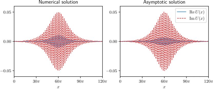
Figure 9: The left panel is the numerical solution of Eq. 4, reproduced from Fig. 4(c). The right panel shows the asymptotic solution, given in Eq. 34. These solutions are at $F=0.073$.

In Fig. 9, we compare the asymptotic solution Eq. 34 with the localized solution from Eq. 4 which we found numerically in Section 2. The similarity betwen the two is quite striking; the main difference is that the real part of the asymptotic solution is somewhat smaller than that of the numerically computed solution, indicating a small error in the phase $\phi$.

At this order, we do not find a connection between the position of the sech envelope and that of the underlying $\cos(k_{c}x)$ pattern. The relative position should not be arbitrary, and could presumably be determined using an asymptotic beyond-all-orders theory [11].

6 Discussion

In this article, we have shown the existence of oscillons in the PDE Eq. 4, which was proposed as a pheonomenological model for the Faraday wave experiments in [34]. We first used numerical simulation, and found that straightforward time-stepping with carefully chosen parameter values and initial conditions leads to a stable oscillon solution, as shown in Fig. 2. We then turned to analysis. Assuming that the damping, detuning and forcing are weak and that the group velocity and amplitude are small, we reduced the PDE Eq. 4 to the coupled forced complex Ginzburg–Landau (FCGL) equations Eq. 14. We stress that we do not get a single FCGL equation with an $\bar{A}$ term, cf. Eq. 3, which is commonly used as a starting point in discussions of oscillons in parametrically forced systems [4, 16, 30]. The single FCGL equation is appropriate when there is a zero-wavenumber bifurcation [2] or if the group velocity is zero. However, if the wavenumber is nonzero (as in Faraday waves) and the group velocity is nonzero but small, the coupled FCGL equations should be used. The coupled FCGL equations, and the model PDE, both exhibit snaking behaviour though the snaking region is very narrow.

Under the further assumption that the strength of the forcing is close to the onset of instability, we then reduced the coupled FCGL equations to the subcritical real Ginzburg–Landau equation Eq. 32. This equation has a sech solution, which, after undoing the reductions, yields an approximate expression for the oscillon, cf. Eq. 34. This expression agrees well with the oscillon found numerically (see Fig. 9), just as was found in [2], where we studied a zero-wavenumber version of this problem.

One special feature of our model PDE Eq. 4 is that the linear terms lead only to positive-frequency oscillations: $U\sim e^{it}$. With spatial dependence, we have left-travelling and right-travelling waves, see Eq. 5. In the Faraday wave experiment, as described by the Zhang–Viñals equations [43] or the Navier–Stokes equations [36], the PDEs are real and so both positive and negative frequency travelling waves can be found. Topaz and Silber [38] wrote down amplitude equations for these travelling waves in the context of two-frequency forcing, without long length scale modulation. In spite of having only positive frequency, our coupled FCGL equations (with spatial modulation removed) have the same form as the travelling wave amplitude equations in [38] (after truncation to cubic order). These travelling wave equations (without modulation terms) can similarly be reduced to standing wave equations [32, 38] with a phase relationship like Eq. 25 between the complex amplitudes of the travelling wave components. Therefore, we expect that the fact that the model PDE Eq. 4 has $e^{it}$ dominant should not prevent oscillons being found by the same mechanism in PDEs that are closer to the fluid dynamics, because our model PDEs and PDEs for fluid mechanics lead to the same amplitude equation in the absence of spatial modulation.

Since [32, 38] did not include spatial modulations, they did not have to consider the group velocity. In the present study, we assumed that the group velocity is small, of the same order as the amplitude of the solution, in order to make progress. This assumption is questionable in the context of fluid mechanics. It would be better to assume that the group velocity is order one, as in [27]. In that case, the left-travelling wave sees only the average of the right-travelling wave and vice versa, leading to (nonlocal) averaged equations. The authors of [27] found spatially uniform and non-uniform solutions with both simple and complex time dependence, but did not study spatially localized solutions. Bringing in spatially localized solutions will be the subject of future work. It is possible to go directly from the PDE Eq. 4 to the real Ginzburg–Landau equation [1, 34], and we expect to be able to do a simular reduction for the Zhang–Viñals or the Navier–Stokes equation for fluid mechanics; cf. [36, 43].

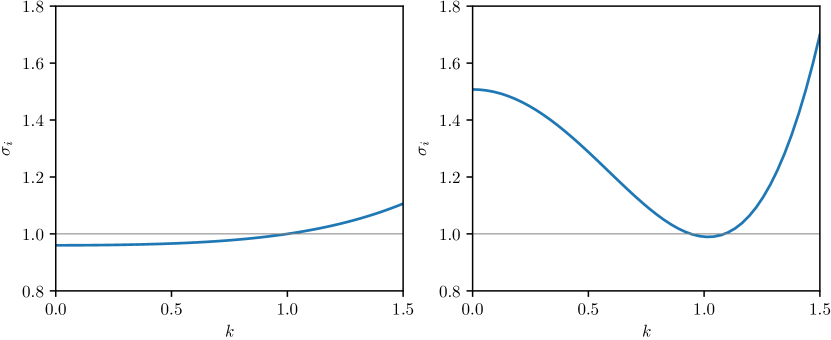
Figure 10: Left panel: The dispersion relation for the PDE model Eq. 4 with $\omega=0.96$, $\beta=-0.02$ and $\delta=0.02$. The frequency $\sigma_{i}(k)$ is close to $1$ over a wide range of $k$. Right panel: Dispersion relation for $\omega=1.5075$, $\beta=1$ and $\delta=0.4825$. Now, $\sigma_{i}(k)$ is equal to $1$ at two distinct wavenumbers.

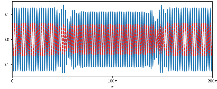
Figure 11: Solution of the PDE model Eq. 4 with two wavenumbers. The parameter values are $\mu=-0.255$, $\omega=1.5075$, $\alpha=-0.5$, $\beta=1$, $\gamma=-0.25$, $\delta=0.4825$, $C=-1-2.5i$ and $F=0.15$.

In the model PDE Eq. 4, when the group velocity is small, waves with a wide range of wavenumbers may be excited. Figure 10 shows two ways in which we can get a fairly small group velocity. The dispersion curve in the left panel is shallow; in this case many wavenumbers are close to resonant ($\sigma_{i}$ is close to $1$). Another possibility is to have two resonant wavenumbers around $k=1$, so that $\sigma_{i}$ is close to a minimum (where $v_{g}=0)$ at $k=1$; see the right panel for an example. In the latter case, solutions with two nearby wavelengths can be expected. Indeed, we did observe such solutions in the PDE model Eq. 4; an example is given in Fig. 11. These states resemble those found by Bentley [7] in an extended Swift–Hohenberg model, and by Riecke [33] in the coupled FCGL equations with small group velocity in the supercritical case.

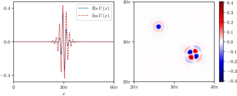
Figure 12: Strongly localized oscillons in the PDE model Eq. 4 in one (left) and two (right) dimensions with $\mu=-0.375$, $\omega=1.99$, $\alpha=-0.5$, $\beta=1$, $\gamma=-0.25$, $\delta=0.4975$, $C=-1-2.5i$ and $F=1.5$. The right panel shows the real part of $U$ on only part of the domain $[0,60\pi]\times[0,60\pi]$.

Finally, we have throughout kept our paramter $\epsilon$ small ($\epsilon=0.1$), which is why the oscillons in e.g. Fig. 4 are so broad, in contrast to the oscillons seen in experiments (see Fig. 1). As a preliminary exploration of increasing $\epsilon$, we set $\epsilon=0.5$, and, after some minor changes to the parameters, we found strongly localized oscillons in one and two dimensions (see Fig. 12). As the picture in two dimensions shows, it is possible for a solution to contain multiple oscillons, which may or may not be axisymmetric. Reference [1] investigates a related PDE: Eq. 4 but with strong damping and with cubic–quintic (rather than simply cubic) nonlinearity, where the coefficient of the cubic term has positive real part in order to make the oscillons more nonlinear. In this case, snaking was found in both one and two dimensions.

References

- [1] A. S. Alnahdi, Oscillons: localized patterns in a periodically forced system, PhD thesis, University of Leeds (2015).
- [2] A. S. Alnahdi, J. Niesen and A. M. Rucklidge, Localized patterns in periodically forced systems, SIAM J. Appl. Dynam. Systems, 13 (2014), pp. 1311–1327.
- [3] I. S. Aranson and L. S. Tsimring, Domain walls in wave patterns, Phys. Rev. Lett. 75 (1995), pp. 3273–3276.
- [4] I. S. Aranson and L. S. Tsimring, Formation of periodic and localized patterns in an oscillating granular layer, Phys. A, 249 (1998), pp. 103–110.
- [5] H. Arbell and J. Fineberg, Temporally harmonic oscillons in Newtonian fluids, Phys. Rev. Lett., 85 (2000), pp. 756–759.
- [6] T. B. Benjamin and F. Ursell, The stability of the plane free surface of a liquid in vertical periodic motion, Philos. Trans. R. Soc. Lond. A, 225 (1954), pp. 505–515.
- [7] D. C. Bentley, Localised solutions in the magnetorotational Taylor–Couette flow with a quartic marginal stability curve, PhD thesis, University of Leeds (2012).
- [8] C. Bizon, M. D. Shattuck, J. B. Swift, W. D. McCormick and H. L. Swinney, Patterns in 3d vertically oscillated granular layers: simulation and experiment, Phys. Rev. Lett., 80 (1998), pp. 57–60.
- [9] J. Burke and E. Knobloch, Homoclinic snaking: structure and stability, Chaos, 17 (2007), 037102.
- [10] J. Burke, A. Yochelis and E. Knobloch, Classification of spatially localized oscillations in periodically forced dissipative systems, SIAM J. Appl. Dynam. Systems, 7 (2008), pp. 651–711.
- [11] S. J. Chapman and G. Kozyreff, Exponential asymptotics of localised patterns and snaking bifurcation diagrams, Phys. D, 238 (2009), pp. 319–354.
- [12] S. M. Cox and P. C. Matthews, Exponential time differencing for stiff systems, J. Comput. Phys., 176 (2002), pp. 430–455.
- [13] C. Crawford and H. Riecke, Oscillon-type structures and their interaction in a Swift–Hohenberg model, Phys. D, 129 (1999), pp. 83–92.
- [14] J. H. P. Dawes, Localized pattern formation with a large-scale mode: Slanted snaking, SIAM J. Appl. Dynam. Systems, 7 (2008), pp. 186–206.
- [15] J. H. P. Dawes, The emergence of a coherent structure for coherent structures: localized states in nonlinear systems, Philos. Trans. R. Soc. Lond. A, 368 (2010), pp. 3519–3534.
- [16] J. H. P. Dawes and S. Lilley, Localized states in a model of pattern formation in a vertically vibrated layer, SIAM J. Appl. Dynam. System, 9 (2010), pp. 238–260.
- [17] S. P. Decent and A. D. D. Craik, Hysteresis in Faraday resonance, J. Fluid Mech., 293 (1995), pp. 237–268.
- [18] E. J. Doedel, AUTO-07P: Continuation and bifurcation software for ordinary differential equations, 2012.
- [19] W. S. Edwards and S. Fauve, Patterns and quasi-patterns in the Faraday experiment, J. Fluid Mech., 278 (1994), pp. 123–148.
- [20] M. Faraday, On a peculiar class of acoustical figures; and on certain forms assumed by groups of particles upon vibrating elastic surfaces, Philos. Trans. R. Soc. Lond., 121 (1831), pp. 299–340.
- [21] R. B. Hoyle, Pattern Formation: An introduction to methods, Cambridge University Press (2006).
- [22] E. Knobloch, Spatial localization in dissipative systems, Annu. Rev. Condens. Matter Phys., 6 (2015), pp. 325–359.
- [23] J. Lega, J. V. Moloney, and A. C. Newell, Swift–Hohenberg equation for lasers, Phys. Rev. Lett., 73 (1994), pp. 2978–2981.
- [24] O. Lioubashevski, H. Arbell and J. Fineberg, Dissipative solitary states in driven surface waves, Phys. Rev. Lett., 76 (1996), pp. 3959–3962.
- [25] O. Lioubashevski, Y. Hamiel, A. Agnon, Z. Reches, and J. Fineberg, Oscillons and propagating solitary waves in a vertically vibrated colloidal suspension, Phys. Rev. Lett., 83 (1999), pp. 3190–3193.
- [26] S. Longhi, Spatial solitary waves in nondegenerate optical parametric oscillators near an inverted bifurcation, Opt. Commun., 149 (1998), pp. 335–340.
- [27] C. Martel, E. Knobloch, J. M. Vega, Dynamics of counterpropagating waves in parametrically forced systems, Phys. D, 137 (2000), pp. 94–123.
- [28] Y.-P. Ma, J. Burke and E. Knobloch, Defect-mediated snaking: A new growth mechanism for localized structures, Phys. D, 239 (2010), pp. 1867–1883.
- [29] I. Melbourne, Derivation of the time-dependent Ginzburg–Landau equation on the line, J. Nonlin. Sci., 8 (1998), pp. 1–15.
- [30] K. McQuighan and B. Sandstede, Oscillons in the planar Ginzburg–Landau equation with 2:1 forcing, Nonlinearity, 27 (2014), pp. 3073–3116.
- [31] V. Petrov, Q. Ouyang and H. Swinney, Resonant pattern formation in a chemical system, Nature, 388 (1997), pp. 655–657.
- [32] J. Porter and M. Silber, Resonant triad dynamics in weakly damped Faraday waves with two-frequency forcing, Phys. D, 190 (2004), pp. 93–114.
- [33] H. Riecke, Stable wave-number kinks in parametrically excited standing waves, Europhys. Lett., 11 (1990), pp. 213–218.
- [34] A. M. Rucklidge and M. Silber, Design of parametrically forced patterns and quasipatterns, SIAM J. Appl. Dyn. Syst., 8 (2009), pp. 298–347.
- [35] M. Shats, H. Xia and H. Punzmann, Parametrically excited water surface ripples as ensembles of oscillons, Phys. Rev. Lett., 108 (2012), 034502.
- [36] A. C. Skeldon and G. Guidoboni, Pattern selection for Faraday waves in an incompressible viscous fluid, SIAM J Appl. Math., 67 (2007), pp. 1064–1100.
- [37] L. Tsimring and I. Aranson, Localized and cellular patterns in a vibrated granular layer, Phys. Rev. Lett., 79 (1997), pp. 213–216.
- [38] C. M. Topaz and M. Silber, Resonances and superlattice pattern stabilization in two-frequency forced Faraday waves, Phys. D, 172 (2002), pp. 1–29.
- [39] P. B. Umbanhowar, F. Melo and H. L. Swinney, Localized excitations in a vertically vibrated granular layer, Nature, 382 (1996), pp. 793–796.
- [40] J. Wu, R. Keolian and I. Rudnick, Observation of a non-propagating hydrodynamic soliton, Phys. Rev. Lett., 52 (1984), pp. 1421–1424.
- [41] A. Yochelis, J. Burke and E. Knobloch, Reciprocal oscillons and nonmonotonic fronts in forced nonequilibrium systems, Phys. Rev. Lett., 97 (2006), 254501.
- [42] W. Zhang and J. Viñals, Secondary instabilities and spatiotemporal chaos in parametric surface waves, Phys. Rev. Lett., 74 (1995), pp. 690–693.
- [43] W. Zhang and J. Viñals, Pattern formation in weakly damped parametric surface waves, J. Fluid Mech., 336 (1996), pp. 301–330.