Recovery schemes for primitive variables in
general-relativistic magnetohydrodynamics

Abstract

General-relativistic magnetohydrodynamic (GRMHD) simulations are an important tool to study a variety of astrophysical systems such as neutron star mergers, core-collapse supernovae, and accretion onto compact objects. A conservative GRMHD scheme numerically evolves a set of conservation equations for ’conserved’ quantities and requires the computation of certain primitive variables at every time step. This recovery procedure constitutes a core part of any conservative GRMHD scheme and it is closely tied to the equation of state (EOS) of the fluid. In the quest to include nuclear physics, weak interactions, and neutrino physics, state-of-the-art GRMHD simulations employ finite-temperature, composition-dependent EOSs. While different schemes have individually been proposed, the recovery problem still remains a major source of error, failure, and inefficiency in GRMHD simulations with advanced microphysics. The strengths and weaknesses of the different schemes when compared to each other remain unclear. Here we present the first systematic comparison of various recovery schemes used in different dynamical spacetime GRMHD codes for both analytic and tabulated microphysical EOSs. We assess the schemes in terms of (i) speed, (ii) accuracy, and (iii) robustness. We find large variations among the different schemes and that there is not a single ideal scheme. While the computationally most efficient schemes are less robust, the most robust schemes are computationally less efficient. More robust schemes may require an order of magnitude more calls to the EOS, which are computationally expensive. We propose an optimal strategy of an efficient three-dimensional Newton–Raphson scheme and a slower but more robust one-dimensional scheme as a fall-back.

1 Introduction

Magnetized plasmas in gravitating systems where general relativity is important play a pivotal role in understanding a variety of phenomena across astrophysics, including accreting black holes in (X-ray) binaries and active galactic nuclei, short and long gamma-ray bursts, core-collapse supernovae, and compact-object mergers involving neutron stars. Various general-relativistic magnetohydrodynamic (GRMHD) codes have been developed to study these systems from first principles, both in stationary background spacetime (e.g., HARM (Gammie et al., 2003); Komissarov 2005; Antón et al. 2006; ECHO (Del Zanna et al., 2007); Athena++ (White et al., 2016)) and in fully dynamical spacetime (e.g., Duez et al. 2005; WhiskyMHD (Giacomazzo & Rezzolla, 2007); Cerdá-Durán et al. 2008; Anderson et al. 2008; Kiuchi et al. 2012; GRHydro (Mösta et al., 2014a); SpEC (Muhlberger et al., 2014); IllinoisGRMHD (Etienne et al., 2015)).

Conservative GRMHD schemes, such as the ones employed by the aforementioned codes, solve the equations of GRMHD as a set of conservation equations of the form (see Sec. 2)

$$\partial_{t}(\sqrt{\gamma}\mathbf{q})+\partial_{i}[\alpha\sqrt{\gamma}\mathbf{f}^{(i)}(\mathbf{p})]=\mathbf{s}(\mathbf{p}),$$ (1)

where $\alpha$ and $\gamma$ are (known) quantities derived from the spacetime metric. Here, $\mathbf{q}$ represents a vector of so-called conserved quantities, which are analytic functions of the so-called primitive variables $\mathbf{p}$, $\mathbf{q}=\mathbf{q}(\mathbf{p})$. Since the fluxes $\mathbf{f}^{(i)}(\mathbf{p})$ and source terms $\mathbf{s}(\mathbf{p})$ are functions of the primitives, at every time step of the conservative scheme, the given vector of conserved variables needs to be inverted to obtain the primitive variables in order to evolve $\mathbf{q}$ to the next time step. This recovery procedure therefore represents a core part of every conservative GRMHD scheme.

Whereas the inversion from conservative to primitive quantities is known in terms of analytical relations in Newtonian MHD and only requires iterative procedures to obtain thermodynamic quantities for a general equation of state (EOS), there is no known inversion in closed form in GRMHD, and usually a set of nonlinear equations needs to be solved to obtain the primitives $\mathbf{p}=\mathbf{p}(\mathbf{q})$. Complication arises from the EOS, which captures the thermodynamic properties of the fluid and which is closely tied to the recovery problem. Most GRMHD codes have used simple analytic EOSs so far, such as (piecewise) polytropic EOS or an ideal-gas EOS, in which case specific recovery schemes exist (Noble et al., 2006). Even in the context of simple analytic and well-behaved EOSs, this recovery problem is one of the most error-prone key parts of any GRMHD evolution code.

Advancing realism in numerical simulations, particularly in fully dynamical spacetime applications such as core-collapse supernovae and compact binary mergers, requires GRMHD codes to support composition-dependent, finite-temperature EOSs, typically formulated in terms of rest-mass density, temperature, and electron fraction (three-parameter EOSs). For example, the inclusion of weak interactions and (approximate) neutrino transport into GRMHD requires such EOSs. Furthermore, capabilities for composition-dependent, finite-temperature EOSs are required for exploring the influence of different EOSs on neutron star mergers; this may provide an important tool for inferring the unknown EOS of nuclear matter at high densities from observations of neutron star mergers by the Laser Interferometer Gravitational-wave Observatory (LIGO) and electromagnetic facilities. To date, only very few GRMHD codes and studies using composition-dependent EOSs exist (e.g., Neilsen et al. 2014; Palenzuela et al. 2015; Mösta et al. 2014b, 2015; Siegel & Metzger 2017, 2018).

Composition-dependent EOSs are usually supplied to the code partially or entirely in the form of tables. EOS calls by the code therefore involve table lookups with interpolation operations, which can be computationally expensive. Widely used recovery schemes that, in principle, support three-parameter EOSs, such as the 2D scheme in Noble et al. (2006) or the recovery scheme in Antón et al. (2006), require additional inversions using the EOS at every iteration step of the scheme from, e.g., specific enthalpy or pressure to temperature, and thus introduce many additional EOS table lookups; this potentially makes the recovery process computationally expensive and introduces many more operations and additional sources of error and/or failure that make the GRMHD scheme less robust.

In this paper, we discuss and compare several recovery schemes that are suitable for composition-dependent, finite-temperature EOSs. Most of the schemes presented here have already been used in GRMHD simulations, in different codes and by different groups. Here, we provide the first comparison of these schemes in a well-defined test setting, i.e., independent of a specific application, and assess these schemes in terms of three cardinal criteria: (i) speed (in terms of the number of iterations and the number of EOS calls needed to converge), (ii) accuracy, and (iii) robustness. We note that if the numerical code employing the recovery schemes discussed here is based on a finite-volume discretization (as is the case for typical GRMHD codes), the recovery methods discussed here are second-order accurate; additional complexity would arise for higher-order finite-volume schemes.

This paper is organized as follows. Section 2 defines the recovery problem and Sec. 3 introduces the recovery schemes considered in this analysis. Results of our comparison are presented in Sec. 4 and Sec. 5 summarizes our conclusions.

2 The recovery problem

The equations of ideal GRMHD include energy and momentum conservation, baryon number conservation, lepton number conservation, and Maxwell’s equations (e.g., Antón et al. 2006),

$$\nabla_{\mu}T^{\mu\nu} = Qu^{\nu},$$ (2)

$$\nabla_{\mu}(n_{\mathrm{b}}u^{\mu}) = 0,$$ (3)

$$\nabla_{\mu}(n_{\mathrm{e}}u^{\mu}) = R,$$ (4)

$$\nabla_{\nu}F^{*\mu\nu} = 0$$ (5)

where $T^{\mu\nu}$ is the energy–momentum tensor, $u^{\mu}$ the 4-velocity, $n_{\mathrm{b}}$ the baryon number density, $n_{\mathrm{e}}$ the electron number density, and $F^{*\mu\nu}$ the dual of the Faraday electromagnetic tensor. The energy–momentum tensor in ideal GRMHD can be written as

$$T^{\mu\nu}=\left(\rho h+b^{2}\right)u^{\mu}u^{\nu}+\left(p+\frac{b^{2}}{2}\right)g^{\mu\nu}-b^{\mu}b^{\nu},$$ (6)

where $p$ denotes pressure, $h=1+\epsilon+p/\rho$ specific enthalpy, with $\epsilon$ being the specific internal energy, and $b^{\mu}\equiv(4\pi)^{-\frac{1}{2}}F^{*\mu\nu}u_{\nu}$ the magnetic field vector in the frame comoving with the fluid, $b^{2}\equiv b^{\mu}b_{\mu}$, and $g_{\mu\nu}$ the space-time metric. We assume that the thermodynamic properties of matter can be described by a composition-dependent, finite-temperature EOS, formulated as a function of density $\rho=n_{\mathrm{b}}m_{\mathrm{b}}$, where $m_{\mathrm{b}}$ denotes the baryon mass, temperature $T$, and electron fraction $Y_{e}=n_{\mathrm{e}}n_{\mathrm{b}}^{-1}$. Accordingly, we have added an evolution equation for the electron fraction (Eq. (4)) to the original set of ideal GRMHD evolution equations (2), (3), and (5). The terms on the right of Eqs. (2) and (4) represent source terms that reflect the evolution of the electron fraction due to weak interactions, which lead to the emission of neutrinos and antineutrinos that carry away energy and momentum from the system.

For numerical evolution, we adopt a 3+1 split of spacetime into non-intersecting spacelike hypersurfaces of constant coordinate time $t$ (Lichnerowicz, 1944; Arnowitt et al., 2008), writing the line element as

$$\mathrm{d}s^{2}=-\alpha^{2}\mathrm{d}t^{2}+\gamma_{ij}(\mathrm{d}x^{i}+\beta^{i}\mathrm{d}t)(\mathrm{d}x^{j}+\beta^{j}\mathrm{d}t),$$ (7)

where $\alpha$ denotes the lapse function, $\beta^{i}$ the shift vector, and $\gamma_{ij}$ the metric induced on every spatial hypersurface. The hypersurfaces are characterized by the timelike unit normal $n^{\mu}$, where $n^{\mu}=(\alpha^{-1},-\alpha^{-1}\beta^{i})$ and $n_{\mu}=(-\alpha,0,0,0)$. We adopt an Eulerian formulation of the equations of GRMHD in terms of the Eulerian observer, defined as the observer in the 3+1 foliation of spacetime moving with 4-velocity $n^{\mu}$ perpendicular to the hypersurfaces of constant coordinate time $t$.

In this 3+1 decomposition of spacetime and adopting the Eulerian observer, Eqs. (2)–(5) can be reformulated as a set of conservation equations of the form

$$\partial_{t}(\sqrt{\gamma}\mathbf{q})+\partial_{i}[\alpha\sqrt{\gamma}\mathbf{f}^{(i)}(\mathbf{p},\mathbf{q})]=\mathbf{s}(\mathbf{p}),$$ (8)

suitable for numerical evolution. Here, $\gamma$ is the determinant of the spatial metric $\gamma_{ij}$ and

$$\mathbf{q}\equiv[D,S_{i},\tau,B^{i},DY_{e}]$$ (9)

denotes the vector of conserved variables, where

$$D \equiv \rho W$$ (10)

$$S_{i} \equiv -n_{\mu}T^{\mu}_{\phantom{\mu}i}=\alpha T^{0}_{\phantom{0}i}=(\rho h+b^{2})W^{2}v_{i}-\alpha b^{0}b_{i}$$ (11)

$$\tau \equiv n_{\mu}n_{\nu}T^{\mu\nu}-D=\alpha^{2}T^{00}-D$$ (12)

$$= (\rho h+b^{2})W^{2}-\left(p+\frac{b^{2}}{2}\right)-\alpha^{2}(b^{0})^{2}-D,$$ (13)

and $B^{i}$ are the 3-vector components of the magnetic field $B^{\mu}\equiv(4\pi)^{-\frac{1}{2}}F^{*\mu\nu}n_{\nu}$ as measured by the Eulerian observer; $D$ is called the conserved density, $S_{i}$ represent the conserved momenta, and $\tau$ is the conserved energy. For further reference, we note that

$$S^{2} \equiv S^{i}S_{i}$$ (14)

$$= (\rho h+b^{2})^{2}W^{4}v^{2}+\alpha^{2}(b^{0})^{2}$$

$$\times\left[b^{2}(1-2W^{2})-2\rho hW^{2}+\alpha^{2}(b^{0})^{2}\right].$$

The Eulerian observer measures the fluid 4-velocity $u^{\mu}=(u^{0},u^{i})$ with corresponding 3-velocity

$$v^{i}\equiv\frac{\gamma^{i}_{\phantom{i}\mu}u^{\mu}}{-u^{\mu}n_{\mu}}=\frac{u^{i}}{W}+\frac{\beta^{i}}{\alpha},\mskip 20.0muv_{i}=\frac{\gamma_{i\mu}u^{\mu}}{-u^{\mu}n_{\mu}}=\frac{u_{i}}{W},$$ (15)

where

$$W\equiv-u^{\mu}n_{\mu}=\alpha u^{0}=\frac{1}{\sqrt{1-v^{2}}}$$ (16)

is the relative Lorentz factor between $u^{\mu}$ and $n^{\mu}$, with $v^{2}\equiv\gamma_{ij}v^{i}v^{j}$. We note that the comoving and Eulerian magnetic field components are related by

$$b^{i} = \frac{B^{i}}{W}+b^{0}(\alpha v^{i}-\beta^{i}),$$ (17)

$$b_{i} = \frac{B_{i}}{W}+\alpha b^{0}v_{i},$$ (18)

$$b^{0} = \frac{W}{\alpha}B^{i}v_{i},$$ (19)

and

$$b^{2}=b^{\mu}b_{\mu}=\frac{B^{2}+(\alpha b^{0})^{2}}{W^{2}},$$ (20)

where $B^{2}\equiv B^{i}B_{i}$. Furthermore, we shall refer to

$$\mathbf{p}\equiv[\rho,v^{i},\epsilon,B^{i},Y_{e}]$$ (21)

as the vector of primitive variables.

Conservative numerical GRMHD schemes evolve the state vector $\mathbf{q}$ from one time step to the next using Eq. (8). This involves computing the flux terms $\mathbf{f}^{(i)}(\mathbf{p},\mathbf{q})$ and source terms $\mathbf{s}(\mathbf{p})$ for given $\mathbf{q}$, for which one needs to obtain the primitive variables $\mathbf{p}$ from the conserved ones. While the conservative variables as a function of primitive variables, $\mathbf{q}=\mathbf{q}(\mathbf{p})$, are given in analytic form by Eqs. (10)–(20), the inverse relation $\mathbf{p}=\mathbf{p}(\mathbf{q})$, i.e., the recovery of primitive variables from conservative ones, is not known in closed form; this rather requires numerical inversion of the aforementioned set of nonlinear equations.

3 Recovery schemes

The recovery problem is, in principle, five-dimensional (5D), i.e., obtaining the primitives $\rho$, $v^{i}$, $\epsilon$ in Eq. (21) from Eqs. (10)–(20) involves numerical root-finding in a 5D space, given that the recovery of the magnetic field components and the electron fraction from $\mathbf{q}$ (see Eq. (9)) is trivial. While 5D schemes as originally implemented in, e.g., the HARM code (Gammie et al., 2003), were later shown to be slow and inaccurate, reducing the dimensionality of the problem to 1D or 2D with the help of certain scalar quantities proved more efficient, with the 2D schemes being less pathological and therefore being recommended (Noble et al., 2006).

In this section, we first discuss the widely used 2D scheme by Noble et al. (2006) and extend it to three-parameter EOSs, which will serve as a standard reference (hereafter referred to as “2D NR Noble”). We then introduce a variant of the 2D scheme used in Antón et al. (2006), Aasi et al. (2014), Giacomazzo & Rezzolla (2007), and Cerdá-Durán et al. (2008), suitable for the use of three-parameter EOSs (henceforth “2D NR”). Furthermore, we discuss several recovery schemes (3D and effective 1D) that have been proposed recently and that are used in current GRMHD codes with support for composition-dependent, finite-temperature EOSs.

3.1 2D NR Noble et al. scheme

This scheme reduces the dimensionality of the recovery problem by making use of certain scalar quantities that can be computed from the conservatives; it is based on Eqs. (27) and (29) of Noble et al. (2006), which are two equations in the unknowns $z\equiv\rho hW^{2}$ and $v^{2}$. In our notation, they read

$$v^{2}(B^{2}+z)^{2}-\frac{(B^{i}S_{i})^{2}(B^{2}+2z)}{z^{2}}-S^{2}=0,$$ (22)

$$\tau+D-\frac{B^{2}}{2}(1+v^{2})+\frac{(B^{i}S_{i})^{2}}{2z^{2}}\\ -z+p(z,v^{2})=0.$$ (23)

The pressure $p(z,v^{2})$ can be directly obtained in terms of the unknowns $z$ and $v^{2}$ only for simple analytic EOSs such as the ideal-gas EOS. In order to extend this scheme to three-parameter EOSs, at every iteration of the scheme we invert the specific enthalpy $h=z/(\rho W^{2})$ for given $\rho=D/W$, $W=(1-v^{2})^{-1/2}$, and $Y_{e}$ with the help of the EOS to find the temperature $T$ and then compute $p(\rho,T,Y_{e})$ using the EOS. This involves inversion with a 1D Newton–Raphson (NR) scheme, which falls back to bisection if the inversion fails.

Once converged, the final primitives $\rho$, $v^{i}$, and $\epsilon$ can be obtained from $\rho=D\sqrt{1-v^{2}}$,

$$v^{i}=\frac{\gamma^{ij}S_{j}}{z+B^{2}}+\frac{(B^{j}S_{j})B^{i}}{z(z+B^{2})},$$ (24)

and, using the EOS,

$$\epsilon=\epsilon(\rho,T,Y_{e}).$$ (25)

3.2 2D NR scheme

In the following, we present a 2D scheme that starts from the same equations as the 2D schemes in Antón et al. (2006),Giacomazzo & Rezzolla (2007), and Cerdá-Durán et al. (2008) and is similar to Noble et al. (2006), but formulated in terms of unknowns that are more suitable for the use of modern microphysical (tabulated) EOSs provided in terms of $\rho$, $T$, and $Y_{e}$. The advantage of our formulation is that additional inversion steps from specific enthalpy or specific internal energy to temperature are not necessary. Such additional inversions at every iteration of the main root-finding process are not required in the case of the ideal-gas EOS, but introduce additional operations and sources of error or failure for three-parameter EOSs, and are computationally expensive.

Similar to the 2D NR Noble scheme (Sec. 3.1), this scheme reduces the dimensionality of the recovery problem to 2D by making use of the two scalar quantities $\tau$ (see Eq. (13)) and $S^{2}$ (see Eq. (14)). Setting $z\equiv\rho hW^{2}$ as before and using the identity

$$B^{i}S_{i}=\rho hW\alpha b^{0},$$ (26)

one can write Eq. (13) and (14) as

$$\left[\tau+D-z-B^{2}+\frac{(B^{i}S_{i})^{2}}{2z^{2}}+p\right]W^{2}-\frac{B^{2}}{2}=0,$$ (27)

$$\left[(z+B^{2})^{2}-S^{2}-\frac{2z+B^{2}}{z^{2}}(B^{i}S_{i})^{2}\right]W^{2}\\ -(z+B^{2})^{2}=0.$$ (28)

Employing the EOS to compute the pressure from $(\rho,T,Y_{e})$, we take Eqs. (27) and (28) as two equations in the unknowns $W$ and $T$ by setting $z=z(W,T)$, $p=p(W,T)$, with $\rho$ being calculated from Eq. (10), and solve using a 2D NR algorithm. Once converged, the final primitives $\rho,v^{i},\epsilon$ are obtained from Eqs. (10), (24), and (25).

3.3 3D NR scheme

Equations (27) and (28) can be extended to a 3D system in the unknowns $W$, $z$, and $T$ by adding a constraint on the specific internal energy (Cerdá-Durán et al., 2008),

$$\left[\tau+D-z-B^{2}+\frac{(B^{i}S_{i})^{2}}{2z^{2}}+p\right]W^{2}-\frac{B^{2}}{2}=0$$ (29)

$$\left[(z+B^{2})^{2}-S^{2}-\frac{2z+B^{2}}{z^{2}}(B^{i}S_{i})^{2}\right]W^{2}\\ -(z+B^{2})^{2}=0$$ (30)

$$\epsilon-\epsilon(\rho,T,Y_{e})=0.$$ (31)

Here, $\epsilon$ is computed as

$$\epsilon=\epsilon(W,z,T)=h-1-\frac{p}{\rho}=\frac{z-DW-pW^{2}}{DW},$$ (32)

and both $p$ in Eqs. (29) and (32) and $\epsilon(\rho,T,Y_{e})$ in Eq. (31) are computed using the EOS with $\rho$ from Eq. (10). As this scheme also employs the temperature directly as an unknown, it does not require any inversions with the EOS. Once the system of Eqs. (29)–(31) has been solved with a 3D NR scheme, one recovers the final primitives $\rho,v^{i},\epsilon$ from Eqs. (10), (24), and (25).

3.4 effective 1D schemes

3.4.1 Method of Palenzuela et al.

The scheme recently presented by Neilsen et al. (2014) and Palenzuela et al. (2015) reduces the dimensionality of the recovery problem to 1D, but requires an additional inversion step using the EOS at every iteration of the main scheme if the EOS is not provided in terms of $(\rho,\epsilon,Y_{e})$. The scheme utilizes Brent’s method to solve

$$f(x)=x-\hat{h}\hat{W}=x-\left(1+\hat{\epsilon}+\frac{p(\hat{\rho},\hat{\epsilon},Y_{e})}{\hat{\rho}}\right)\hat{W}$$ (33)

in the unknown

$$x\equiv\frac{\rho hW^{2}}{\rho W}=hW,\\$$ (34)

which is bounded by

$$1+q-s<x<2+2q-s.$$ (35)

Here, following Palenzuela et al. (2015), we have defined

$$q \equiv \tau/D,$$ (36)

$$r \equiv S^{2}/D^{2},$$ (37)

$$s \equiv B^{2}/D,$$ (38)

$$t \equiv B_{i}S^{i}/D^{3/2}.$$ (39)

Quantities with a hat in Eq. (33) are computed at every iteration step from $x$ and the conservatives by the following procedure:

• With

  $$S_{i}=(\rho hW^{2}+B^{2})v_{i}-(B_{j}v^{j})B_{i}$$ (40)

  (see Eqs. (11), (19), (20)), using

  $$B^{i}S_{i}=\rho hW^{2}B^{i}v_{i}$$ (41)

  and the definition of $r$ (see Eq. (39)), one can write

  $$\hat{W}^{-2}=1-\frac{x^{2}r+(2x+s)t^{2}}{x^{2}(x+s)^{2}}.$$ (42)

• Using Eq. (10), one obtains $\hat{\rho}=D/\hat{W}$.

• Starting from $\epsilon=h-1-p/\rho$ using Eqs. (19), (20), and (41), one can write

  $$\hat{\epsilon} = -1+\frac{x}{\hat{W}}(1-\hat{W}^{2})$$ (44)

  $$+\hat{W}\left[1+q-s+\frac{1}{2}\left(\frac{t^{2}}{x^{2}}+\frac{s}{\hat{W}^{2}}\right)\right].$$

• Using the EOS, one inverts $\hat{\epsilon}$ to find the corresponding temperature and thus $p(\hat{\rho},\hat{\epsilon},Y_{e})$.

Once converged, the recovered $\rho$ and $\epsilon$ are obtained from Eqs. (10), (42), and (44); the velocity components $v^{i}$ are obtained from Eq. (24) setting $z=x\rho W$.

3.4.2 Method of Newman & Hamlin

The recovery scheme presented in Newman & Hamlin (2014) is an effective 1D method, as is the scheme of Palenzuela et al. (2015) and Neilsen et al. (2014) discussed above. It iterates over the fluid pressure to find a solution, and as in the method of Palenzuela et al. (2015) it requires an additional inversion step using the EOS for every main scheme iteration. It is independent of an initial guess because it starts with $p=0$ as a guess for the pressure. For a tabulated EOS with a finite minimum pressure, we employ the pressure obtained from the minimum temperature of the EOS at given $\rho=D/W$ and $Y_{e}$, where $W$ is an initial guess for the present Lorentz factor.

• Starting from the conserved quantities

  $$e \equiv \tau+D,$$ (45)

  $$S^{i} = [wW^{2}+B^{2}]v^{i}-(B^{i}v_{i})B^{i},$$ (46)

  $$D = \rho W,$$ (47)

  $$\mathcal{M}^{2} = \frac{(B^{i}v_{i})^{2}}{\sqrt{\gamma}},\mathcal{T}=\frac{B^{i}S_{i}}{\sqrt{\gamma}},B^{2},$$ (48)

  where $w=\rho h$, the scheme solves a cubic polynomial

  $$f(\varepsilon)=\varepsilon^{3}+a\varepsilon^{2}+d$$ (49)

  for

  $$\varepsilon\equiv B^{2}+z,\\$$ (50)

  where $z\equiv\rho hW^{2}=wW^{2}$ as before and

  $$a=e+P+\frac{B^{2}}{2},$$ (51)

  $$d=\frac{1}{2}(\mathcal{M}^{2}B^{2}-\mathcal{T}^{2}).$$ (52)

  Evaluating the positive extremum of this equation, one can find a sufficient condition for the existence of a positive root to Eq. (49) as

  $$d\leq\frac{4}{27}4a^{3}.$$ (53)

  Using

  $$d\equiv\frac{4}{27}a^{3}\cos^{2}(\phi)$$ (54)

  one can show that for $0\leq\phi\leq 2\pi$, with

  $$\phi=\arccos\left(\frac{1}{a}\sqrt{\frac{27d}{4a}}\right),$$ (55)

  the first root of

  $$\varepsilon^{(l)}=\frac{1}{3}-\frac{2}{3}a\cos\left(\frac{2}{3}\phi+\frac{2}{3}l\pi\right)$$ (56)

  corresponds to the correct and physical solution of Eq. (49), from which one obtains $z$.

• One can now compute primitive quantities as

  $$v^{2} = \frac{\mathcal{M}^{2}z^{2}+\mathcal{T}^{2}(B^{2}+2z)}{z^{2}(B^{2}+z)^{2}},$$ (57)

  $$W^{2} = \frac{1}{\sqrt{1-v^{2}}},$$ (58)

  $$w = \frac{z}{W^{2}},$$ (59)

  $$\rho = \frac{D}{W}.$$ (60)

  Inverting $w$ with the help of the EOS for $\rho$ of Eq. (60) and given $Y_{e}$, one obtains the corresponding temperature $T$ and a new pressure guess $p$.

• One iterates over steps (i) and (ii) until the pressure has converged. When three successive pressure estimates are known, the Aitken acceleration scheme as described in Newman & Hamlin (2014) is used. If convergence is reached under the Aitken acceleration, we recalculate the variables as in step (ii). If not, the solver restarts from the beginning of step (i).

• Once a converged value for $p$ has been acquired, including a consistent set of $\rho$, $T$, and $\epsilon$ from (iii), the remaining primitives $v^{i}$ can be obtained from Eq. (24).

4 Comparison of recovery schemes

4.1 Comparison setup and criteria

Comparing the different recovery schemes described in Sec. 3 proceeds by generating a parameter space of primitive variables $\mathbf{p}\equiv[\rho,v^{i},\epsilon,B^{i},Y_{e}]$, computing the corresponding conservative variables $\mathbf{q}=\mathbf{q}(\mathbf{p})$ using Eqs. (10)–(13), and applying the recovery schemes to obtain sets of primitives that can be compared to the original ones. We perform this comparison of schemes for three different EOSs—the analytic ideal-gas EOS $p=(\Gamma-1)\rho\epsilon$ (where we arbitrarily set $\Gamma=4/3$), the partially analytic, partially tabulated Helmholtz EOS (Timmes & Arnett, 1999; Timmes & Swesty, 2000) with modifications as described in Siegel & Metzger (2017), and the fully tabulated Lattimer–Swesty EOS (Lattimer & Swesty, 1991) with incompressibility modulus $K=220\,\mathrm{MeV}$ (hereafter LS220), which serves as a widely used standard reference EOS in GRMHD simulations of neutron star mergers and core-collapse supernovae. We reduce the parameter space by varying the Lorentz factor $W$ instead of $v^{i}$, and then choosing the orientation of the 3-velocity randomly at every point in the parameter space. The magnetic field vector is set by a specified absolute value and oriented relative to the 3-velocity vector by a specified angle. For the results presented below, we shall assume that $B^{i}$ and $v^{i}$ are aligned for simplicity; the results for the comparison of the schemes do not depend strongly on this relative orientation. For those recovery schemes that require initial guesses explicitly (such as 2D NR Noble, 2D NR, 3D NR) or implicitly (such as 1D Brent), we apply a $5\%$ random perturbation to the initial primitives and use the perturbed set as the initial guess; this $5\%$ deviation typically represents a conservative bracket on the change from one time step to the next in an actual GRMHD evolution and should thus lead to a conservative upper limit on, e.g., the number of iterations or EOS calls required to converge to the solution. We have checked that the results presented here are essentially unchanged if an even higher perturbation of 10% is applied. If the recovery fails in the case of 2D NR and 3D NR, we use the “safe guess” initial values of Cerdá-Durán et al. (2008) in a second recovery attempt. We define convergence of a scheme by having surpassed a $\mathrm{tol}_{\mathrm{conv}}=5\times 10^{-9}$ (maximum) relative error in the iteration variable(s). The resulting recovered primitives are compared to the original set and to the results from the other recovery schemes in terms of the following criteria.

• Speed. The speed of a given recovery scheme is assessed by counting the number of iterations needed to converge to a solution. Additionally, we have implemented counters to evaluate the total number of EOS calls required until convergence. As table lookups can dominate the computational cost of the recovery scheme and with some schemes requiring additional EOS inversion steps at each iteration, monitoring the number of EOS calls represents a better proxy for the overall speed of a scheme than just counting the number of iterations.

• Accuracy. We assess the accuracy of recovery by comparing the recovered primitives $\mathbf{p}$ with the original ones $\mathbf{p}_{\mathrm{or}}$ and computing the mean relative deviation/error,

  $$\mathrm{tol}_{\mathrm{recov}}\equiv\frac{1}{5}\sum_{i=1}^{5}\Big{|}\frac{\mathbf{p}_{i}-\mathbf{p}_{\mathrm{or},i}}{\mathbf{p}_{\mathrm{or},i}}\Big{|},$$ (61)

  where only $\rho$, $v^{i}$, and $\epsilon$ are included in the summation, because $B^{i}$ and $Y_{e}$ are recovered trivially. We define successful recovery of the primitives as when all primitives have been recovered with a relative error smaller than $\mathrm{tol}_{\mathrm{recov}}=10\times\mathrm{tol}_{\mathrm{conv}}$.

• Robustness. Robustness is assessed qualitatively in terms of the following criteria: independence of an initial guess, guaranteed convergence, and independence of thermodynamic derivatives.

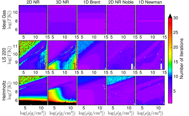
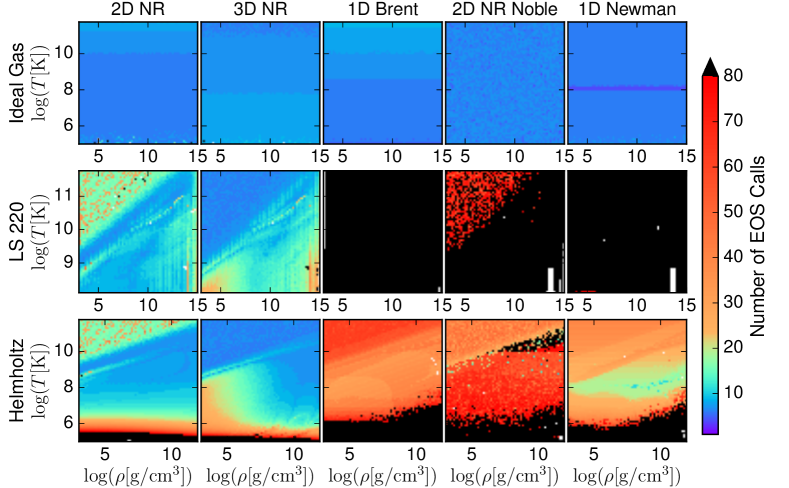
Figure 1: Comparison of schemes in terms of the number of iterations (top) and number of EOS calls (bottom) required for convergence. This set of comparison assumes a Lorentz factor of $W=2$, magnetic to fluid pressure ratio of $p_{\mathrm{mag}}/p=10^{-3}$, and an electron fraction of $Y_{e}=0.1$.

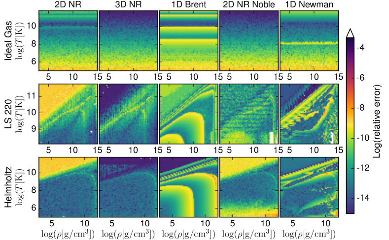
Figure 2: Comparison of schemes in terms of the relative accuracy obtained in recovering the primitive variables, for the same set of parameters as in Fig. 1, i.e., $W=2$, $p_{\mathrm{mag}}/p=10^{-3}$, $Y_{e}=0.1$.

4.2 Results

Figures 1–3 show comparisons of the five different recovery schemes discussed in this paper. We present results for three different EOSs—the ideal-gas EOS, the LS220 tabulated EOS, and the partially tabulated Helmholtz EOS. White spaces correspond to parameter sets for which the recovery process either failed or did not achieve the required accuracy $\mathrm{tol}_{\mathrm{recov}}$ (Sec. 4.1) within a certain number of iterations.

The top panels of Fig. 1 compare the number of iterations required for each scheme to converge to the correct primitive variables within the required accuracy $\mathrm{tol}_{\mathrm{conv}}$ (Sec. 4.1). The parameter range in density $\rho$ and temperature $T$ is chosen to cover the validity ranges of the chosen EOS and we assume representative values of $W=2$ and $p_{\mathrm{mag}}/p=10^{-3}$, where $p_{\mathrm{mag}}=b^{2}/2$ is the magnetic pressure.

For the ideal-gas EOS, all schemes recover the entire parameter space in density and temperature with only a few iterations ($\sim 5$). The 2D NR Noble scheme overall requires the smallest number of iterations.

For the LS220 EOS there is more variation among the different schemes. The 2D NR scheme recovers most of the parameter space with $\lesssim\!10$ iterations but requires 15–30 iterations in the upper left corner as well as for densities above $\sim\!10^{12}\,\mathrm{g\,cm^{-3}}$ and temperatures below $\log T=10.5\,\mathrm{K}$. The 3D NR scheme needs 15–25 iterations for regions at lower temperature, whereas the 1D Brent method performs well and recovers the entire parameters space with $\lesssim\!10$ iterations. The 2D NR Noble and 1D Newman methods perform similarly with the exception that there are small regions where the schemes do not recover the primitives within the given accuracy at very high density and low temperature (white pixels in the bottom right corners). These points account for less than 1.5% of the total points. These failures arise because the additional inversion step of finding a temperature for the given relativistic enthalpy fails in the EOS table. We have investigated this in some detail and find that for all of these points the initial first step in the solver leads to relativistic enthalpy values outside of the EOS table. We have implemented a limitation on step size for these cases but did not find a straightforward way to successfully apply it consistently to all points without additional side effects. While there are a number of ways in which a more sophisticated treatment of step sizes can be implemented, we have chosen to not fine-tune inversions for individual schemes too much with respect to others in order to ensure a fair comparison. The requirement of this additional inversion for temperature given the relativistic enthalpy is a feature/weakness of these schemes that limits their robustness.

For the Helmholtz EOS, the 2D and 3D NR solvers recover most of the parameter space with less than 10 iterations. Both solvers, however, need $\geq\!30$ iterations for very low temperatures. The 2D NR solver additionally needs $\gtrsim\!15$ iterations in the upper left corner. The extent of this region is similar to the results of the 2D NR solver for the LS220 EOS. The 1D Brent, 2D NR Noble, and 1D Newman methods recover the correct solution with fewer than 10–12 iterations in the entire parameter space.

Based on the number of iterations to converge, the 1D Brent method would be one obvious first choice because it recovers the entire parameter space for all EOSs well with $\leq\!10$ iterations.

In the bottom panels of Fig. 1, we show the number of EOS calls for each recovery scheme and the same three EOSs as in the top panels. While there is no drastic variation in the number of iterations to convergence for the different schemes, the number of EOS calls required by the different schemes varies dramatically. All schemes need a small number ($<10$) of EOS calls to converge for the ideal-gas EOS. For the LS220 EOS, the 2D and 3D NR schemes need fewer than $\sim\!25$ EOS calls to converge in the entire parameter space. The 1D Brent, 2D NR Noble, and 1D Newman schemes, however, require typically an order of magnitude more EOS calls to converge throughout the entire parameter space (in the region of 500–1000 EOS calls). The color bar is adjusted to enhance the dynamic range for the more efficient schemes. The average number of EOS calls of all test points is summarized in Table 1. These large numbers of EOS calls are due to the fact that the 1D Brent, 2D NR Noble, and 1D Newman schemes each require an additional inversion in the EOS table per solver iteration. Each of these inversions, in turn, typically requires tens of steps to converge and a few EOS calls per step. The results for the Helmholtz EOS are similar to those for LS220, although the absolute numbers of required EOS calls are lower for the 1D Brent, 2D NR Noble, and 1D Newman schemes.

Table 1: Comparison of different recovery schemes for the parameters in Figs. 1 and 2.

EOS	2D NR	3D NR	1D Brent	2D NR Noble	Newman
Iterations:
IG	5.5	5.4	4.8	4.5	4.9
LS220	11.5	9.1	6.9	6.1	6.1
Helm	25.0	16.2	5.7	6.3	5.9
#EOS calls:
IG	6.5	7.4	6.8	6.5	5.9
LS220	13.0	11.3	836	758	331
Helm	28.2	18.2	111	83.4	57.0
Accuracy:
IG	$3.4\times 10^{-12}$	$7.5\times 10^{-13}$	$2.5\times 10^{-11}$	$8.9\times 10^{-13}$	$4.4\times 10^{-12}$
LS220	$7.1\times 10^{-12}$	$1.3\times 10^{-13}$	$1.0\times 10^{-11}$	$1.7\times 10^{-12}$	$6.1\times 10^{-13}$
Helm	$5.9\times 10^{-13}$	$1.7\times 10^{-14}$	$2.3\times 10^{-12}$	$3.7\times 10^{-12}$	$3.9\times 10^{-13}$

Fig. 2 shows the relative error between original and recovered primitive variables after the schemes have converged for the five different schemes and three EOSs presented in Fig. 1. The NR schemes generally perform better in this metric because one or two additional iterations of the solver improve the accuracy by orders of magnitude.

Table 1 summarizes the different metrics (number of iterations, number of EOS calls, and relative accuracy) averaged over all points in the test parameter space for the five recovery schemes and three EOSs tested here. The averaged values well capture the trends evident from Figs. 1 and 2. Judged by the number of iterations, the 1D Brent, 2D NR Noble and Newman methods are the more efficient schemes. However, the opposite is true for the number of EOS calls, in which case these three schemes need up to one or two orders of magnitude more EOS calls on average than the 2D and 3D NR schemes. For the Helmholtz EOS the situation is not as dire as for LS220, and the number of EOS calls increases by a factor of a few relative to the 2D and 3D NR schemes with the 1D Brent, 2D NR Noble, and Newman methods. The NR and Newman schemes reach a higher overall relative accuracy than the 1D Brent method.

Table 2: Comparison of different recovery schemes for the parameters in Fig. 3.

EOS	2D NR	3D NR	1D Brent	2D NR Noble	Newman
Iterations:
IG	6.8	4.1	7.3	4.6	5.0
LS220	7.5	10.3	7.1	4.3	7.1
Helm	9.8	13.5	7.4	4.3	7.0
#EOS calls:
IG	12.1	8.7	9.3	6.6	6.0
LS220	8.5	17.3	877	329	398
Helm	16.3	52.2	86.2	39.7	35.0
Accuracy:
IG	$1.7\times 10^{-13}$	$4.7\times 10^{-14}$	$1.4\times 10^{-11}$	$2.6\times 10^{-13}$	$5.3\times 10^{-13}$
LS220	$3.3\times 10^{-11}$	$3.6\times 10^{-11}$	$2.9\times 10^{-11}$	$1.4\times 10^{-11}$	$2.0\times 10^{-12}$
Helm	$3.3\times 10^{-13}$	$3.6\times 10^{-13}$	$2.2\times 10^{-11}$	$5.8\times 10^{-13}$	$5.9\times 10^{-13}$
% recovered:
IG	56.0	58.7	74.9	75.7	79.1
LS220	52.6	69.1	68.0	60.0	77.1
Helm	56.9	77.3	75.6	65.0	77.4

A comparison of the five different recovery schemes covering the parameter space in Lorentz factor $W$ and the ratio of magnetic to fluid pressure $p_{\textrm{mag}}/p$ is shown in Fig. 3 (analogous to the top panels of Fig. 1). Here we choose a representative temperature of $T=5\,\mathrm{MeV}$ ($5.8\times 10^{10}\,\mathrm{K}$) and a density of $\rho=10^{11}\,\mathrm{g\,cm^{-3}}$. In general, all schemes fail for very strongly magnetized fluid and/or high Lorentz factors. For the ideal-gas EOS, the methods of 1D Brent, 2D NR Noble, and 1D Newman recover most of the parameter space well and with few iterations ($\leq\!10$). However, the 2D and 3D NR methods do not recover the correct solution beyond Lorentz factors of 10. For the LS220 EOS, the situation is similar to the ideal-gas EOS with the exception of the 3D NR method recovering points up to high Lorentz factors of $W\simeq 100$. For the Helmholtz EOS, similar results to those for the LS220 are obtained, with the 3D NR solver now even recovering up to higher Lorentz factors of $W\simeq 10^{2}-10^{3}$. All metrics are summarized in Tab. LABEL:tab:summary_Wp, which shows similar trends to Tab. 1.

Robustness of the schemes involving an NR algorithm (2D NR, 3D NR, 2D NR Noble) is severely limited by the dependence on good initial guesses. These schemes are particularly sensitive to a good initial guess for the velocity components in the regime of high Lorentz factors. Perturbations at the level of 5% in the primitives as considered here cause definite failure for the 2D NR scheme above Lorentz factors of $W\lesssim\!10$ for all EOSs, partial failure in this regime for the 2D NR Noble scheme and the LS220 and Helmholtz EOS, and failure for the 3D NR scheme and the ideal-gas EOS, as well as a drastically increased number of iterations in the case of the LS220 and the Helmholtz EOS (see Fig. 3). Additionally, all schemes centered around an NR algorithm directly involve thermodynamic derivatives, which often must be numerically computed for tabulated EOSs. These derivatives may be thermodynamically inconsistent (i.e., the Maxwell relations may not be satisfied to machine precision) and they may be noisy, which adds additional sources of error or failure that cannot be controlled and may appear quasi-randomly.

Robustness is significantly improved in the 1D Brent and Newman schemes, which do not depend explicitly on either initial guesses or thermodynamic derivatives. In particular, the fact that there are known brackets for the 1D Brent scheme guarantees the existence of a root and convergence of the scheme. However, for three-parameter EOSs, additional inversions from specific internal energy or enthalpy to temperature are required at every iteration step of the respective main scheme, which is typically accomplished via a 1D NR algorithm. This then implicitly introduces dependences on initial guesses and thermodynamic derivatives. As we find here, inversions of specific internal energy (as in the 1D Brent method) can typically be more robust than inversions of the specific enthalpy (as in the 1D Newman scheme; see the above discussion related to Fig. 1). None of the schemes under consideration here is thus entirely independent of initial guesses. However, in contrast to the 1D Brent method, the 1D Newman scheme starts with a well-defined initial guess for the temperature (the minimum temperature for the EOS at given $\rho$ and $Y_{e}$, see Sec. 3.4.2).

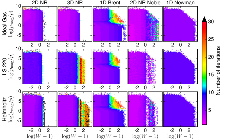
Figure 3: Comparison of schemes in terms of the number of iterations required for convergence. This set of comparisons assumes a density of $\rho=10^{11}\,\mathrm{g}\,\mathrm{cm}^{-3}$, a temperature of $T=5\,\mathrm{MeV}\,(5.8\times 10^{10}\,\mathrm{K})$, and an electron fraction of $Y_{e}=0.1$.

5 Discussion and Conclusion

We performed a comparison of a number of schemes to convert conservative to primitive variables that are used in different GRMHD codes (Sec. 3), employing analytic, partially tabulated, and fully tabulated microphysical EOSs. We have analyzed these methods using a well-defined uniform stand-alone testbed (Sec. 4.1), covering 2D parameter spaces in either density and temperature or Lorentz factor and ratio of magnetic to fluid pressure typically encountered in astrophysical simulations. The schemes are assessed in terms of the three criteria: (i) speed (according to the number of iterations and number of EOS calls required for convergence), (ii) accuracy, and (iii) robustness (Sec. 4.1).

While for the ideal-gas EOS there is not too much variation among the different schemes in terms of speed and accuracy (typically $\leq 10$ iterations and EOS calls), there are significant differences for the microphysical EOSs (LS220 and Helmholtz EOSs; see Tables 1 and LABEL:tab:summary_Wp for a summary). The 2D and 3D NR schemes require 10–20 iterations more to converge in some parts of the parameter space for microphysical EOSs relative to other schemes, but require tens to hundreds of EOS calls fewer and are thus overall much faster. The additional EOS calls in the 1D Brent, 2D NR Noble, and 1D Newman schemes arise because of an additional temperature inversion at every solver iteration that requires roughly 10–100 EOS calls by itself (depending on the inversion scheme and parameters). For tabulated EOSs such as the LS220 and Helmholtz EOSs, the computational cost of a single EOS call can be significant. Therefore, employing the most efficient scheme (3D NR) can yield a speed-up by a factor of at least a few to 10, potentially up to a factor of 100 compared to one of the least efficient schemes. Since the cost of the recovery of primitive variables in an evolution code can be up to $\sim\!40\%$ of the total simulation cost, this can have significant performance impacts on the evolution code, and may determine whether or not a certain simulation is computationally feasible.

The 3D NR scheme clearly emerges as the fastest and most accurate one; however, it is not the most robust scheme. All schemes based on an NR algorithm (2D NR, 3D NR, 2D NR Noble) require good initial guesses and thus do not guarantee convergence. In the case of the 2D NR Noble scheme this can limit the ability to recover at high Lorentz factors (see Fig. 3). When used in an evolution code, these schemes thus depend on the previous time step, which represents a severe limitation that can lead to failure, because data from the previous time step can be corrupted due to numerical error. Furthermore, these schemes explicitly depend on thermodynamic derivatives, which often need to be computed numerically and can thus be noisy and thermodynamically inconsistent. This may lead to failure. The 1D Brent and 1D Newman schemes, however, are both guaranteed to converge and do not explicitly depend on initial guesses and thermodynamic derivatives. However, for microphysical EOSs, additional inversions involving the EOS are required at every solver step, which implicitly introduces dependence on initial guesses (and thermodynamic derivatives, depending on the inversion method). Only the 1D Newman method starts from an independently defined initial guess and is thus entirely independent of the previous time step when used in an evolution code. Furthermore, this additional inversion step may fail and thus limit the robustness of the main scheme. Enthalpy inversions as in the 1D Newman scheme tend to be less robust and more prone to failure (typically at the level of a few per cent in the density–temperature parameter space) than inversions of the specific internal energy as in the 1D Brent scheme.

In conclusion, the optimal recovery scheme for a GRMHD evolution code depends on the EOS. For an analytic EOS, we suggest to employ a more robust scheme such as the 1D Brent or 1D Newman scheme, with the 1D Newman scheme being preferred because it tends to achieve higher accuracy. For microphysical (three-parameter) EOSs, we envision a combination of different schemes. In a first attempt, we suggest to employ the 3D NR scheme, which is both the most efficient and the most accurate scheme among those tested here. For points that fail in this initial pass, one can then switch to a more robust scheme (1D Brent, 1D Newman) in a second step and exploit the greater robustness in the more extreme regions of the parameter space.

An implementation of the recovery schemes discussed in this paper is available as open-source software in Siegel & Mösta (2018). A separate development version is available at https://bitbucket.org/dsiegel/grmhd_con2prim. This code package can be used in GRMHD evolution codes or as a stand-alone framework to add new EOSs and recovery schemes for systematic comparison with existing ones. We value bug reports and code contributions.

References

- Aasi et al. (2014) Aasi, J., Abbott, B. P., Abbott, R., et al. 2014, Phys. Rev. Lett., 113, 011102
- Anderson et al. (2008) Anderson, M., Hirschmann, E. W., Lehner, L., et al. 2008, Phys. Rev. Lett., 100, 191101
- Antón et al. (2006) Antón, L., Zanotti, O., Miralles, J. A., et al. 2006, ApJ, 637, 296
- Arnowitt et al. (2008) Arnowitt, R., Deser, S., & Misner, C. W. 2008, Gen. Rel. Grav., 40, 1997
- Cerdá-Durán et al. (2008) Cerdá-Durán, P., Font, J. A., Antón, L., & Müller, E. 2008, A&A, 492, 937
- Del Zanna et al. (2007) Del Zanna, L., Zanotti, O., Bucciantini, N., & Londrillo, P. 2007, A&A, 473, 11
- Duez et al. (2005) Duez, M. D., Liu, Y. T., Shapiro, S. L., & Stephens, B. C. 2005, Phys. Rev. D, 72, 024028, astro-ph/0503420
- Etienne et al. (2015) Etienne, Z. B., Paschalidis, V., Haas, R., Mösta, P., & Shapiro, S. L. 2015, Class. Quant. Grav., 32, 175009
- Gammie et al. (2003) Gammie, C. F., McKinney, J. C., & Tóth, G. 2003, ApJ, 589, 444
- Giacomazzo & Rezzolla (2007) Giacomazzo, B., & Rezzolla, L. 2007, Class. Quant. Grav., 24, 235
- Kiuchi et al. (2012) Kiuchi, K., Kyutoku, K., & Shibata, M. 2012, Phys. Rev. D, 86, 064008
- Komissarov (2005) Komissarov, S. S. 2005, MNRAS, 359, 801
- Lattimer & Swesty (1991) Lattimer, J. M., & Swesty, F. D. 1991, Nucl. Phys. A, 535, 331
- Lichnerowicz (1944) Lichnerowicz, A. 1944, J. Math. Pures et Appl., 23, 37
- Mösta et al. (2015) Mösta, P., Ott, C. D., Radice, D., et al. 2015, Nature, 528, 376
- Mösta et al. (2014a) Mösta, P., Mundim, B. C., Faber, J. A., et al. 2014a, Class. Quant. Grav., 31, 015005
- Mösta et al. (2014b) Mösta, P., Richers, S., Ott, C. D., et al. 2014b, ApJ, 785, L29
- Muhlberger et al. (2014) Muhlberger, C. D., Nouri, F. H., Duez, M. D., et al. 2014, Phys. Rev. D, 90, 104014
- Neilsen et al. (2014) Neilsen, D., Liebling, S. L., Anderson, M., et al. 2014, Phys. Rev. D, 89, 104029
- Newman & Hamlin (2014) Newman, W. I., & Hamlin, N. D. 2014, SIAM J. Sci. Comput., 36
- Noble et al. (2006) Noble, S. C., Gammie, C. F., McKinney, J. C., & Del Zanna, L. 2006, ApJ, 641, 626
- Palenzuela et al. (2015) Palenzuela, C., Liebling, S. L., Neilsen, D., et al. 2015, Phys. Rev. D, 92, 044045
- Siegel & Metzger (2017) Siegel, D. M., & Metzger, B. D. 2017, Phys. Rev. Lett., 119, 231102
- Siegel & Metzger (2018) —. 2018, ApJ, 858, 52
- Siegel & Mösta (2018) Siegel, D. M., & Mösta, P. 2018, GRMHD_con2prim: a framework for the recovery of primitive variables in general-relativistic magnetohydrodynamics, Zenodo, doi:10.5281/zenodo.1213306. https://doi.org/10.5281/zenodo.1213306
- Timmes & Arnett (1999) Timmes, F. X., & Arnett, D. 1999, ApJS, 125, 277
- Timmes & Swesty (2000) Timmes, F. X., & Swesty, F. D. 2000, ApJS, 126, 501
- White et al. (2016) White, C. J., Stone, J. M., & Gammie, C. F. 2016, ApJS, 225, 22