Probing primordial features with next-generation photometric and radio surveys

Abstract

We investigate the possibility of using future photometric and radio surveys to constrain the power spectrum of primordial fluctuations that is predicted by inflationary models with a violation of the slow-roll phase. We forecast constraints with a Fisher analysis on the amplitude of the parametrized features on ultra-large scales, in order to assess whether these could be distinguishable over the cosmic variance. We find that the next generation of photometric and radio surveys has the potential to test these models at a sensitivity better than current CMB experiments and that the synergy between galaxy and CMB observations is able to constrain models with many extra parameters. In particular, an SKA continuum survey with a huge sky coverage and a flux threshold of a few $\mu$Jy could confirm the presence of a new phase in the early Universe at more than 3$\sigma$.

1 Introduction

Next-generation spectroscopic, photometric and radio galaxy surveys will allow us to map the Universe on the very largest scales – and thus probe the physics of the primordial fluctuations, as well as ultra-large scale general relativistic effects on galaxy observations. Several papers have quantified how well we will be able to constrain primordial non-Gaussianity and relativistic effects in the galaxy power spectrum, using LSST, SKA and other future surveys (see, e.g. [1, 2, 3, 4, 5, 6, 7, 8, 9, 10, 11, 12, 13, 14, 15]).

Another interesting target for future surveys is the possibility to refine our knowledge of the primordial power spectrum and to carefully investigate the statistical significance of the deviations from a simple power law for density fluctuations, that are compatible with the Planck and WMAP CMB temperature power spectrum. These deviations from a simple power law can be easily accommodated in models of inflation with temporary violation of the slow-roll conditions. At present, no inflationary model that fits these features has been found to be preferred at a statistically significant level from CMB data (see, e.g. [16, 17, 18, 21, 20, 22, 23, 24, 25, 26, 27, 19, 28, 29, 30, 31]).

The situation improves if suitable data in addition to the CMB temperature are available. Better CMB E-mode polarization measurements have been highlighted as a possible way to constrain primordial features with high confidence [32, 33]. Galaxy surveys provide a unique opportunity to improve our current understanding about these possible anomalies; see for instance [34, 35, 36, 37, 38, 39, 40, 41, 42, 43].

Here we focus on constraining primordial features using future photometric and radio galaxy surveys that cover a huge volume of the Universe, in order to access the ultra-large scales where primordial features leave an imprint. As examples of such surveys, we use two experiments that are being constructed:

• The Large Synoptic Survey Telescope (LSST) is the widest ($\sim 18,000$ deg²) and deepest ($r_{\rm AB}\sim 27.5$) photometric survey planned in the foreseeable future, with a sample of $\sim 10$ billion galaxies. (See [44].)

• The Square Kilometre Array (SKA) plans to conduct the widest ever spectroscopic surveys, using the 21cm emission line of HI: with intensity mapping in SKA1-MID ($\sim 25,000$ deg² out to $z\sim 3$), and with a galaxy survey in SKA2-MID ($\sim 30,000$ deg², $\sim 1$ billion galaxies out to $z\sim 2$). In addition, using the radio continuum emission, it will detect a huge number of galaxies out to $z\sim 5$, but without redshift information. (See [45, 46, 47, 48].)

The paper is organized as follows. In section 2 we describe the observables, the forecasting methodology and the survey specifications that we used. In section 3 we describe the parametrized features models used in our forecasts. We present our results in section 4 and draw conclusions in section 5.

2 Large-Scale Structure Power Spectra

2.1 Galaxy power spectrum

Galaxies trace the invisible cold dark matter (CDM) distribution and then we can estimate the matter power spectrum and extract information on the underlying power spectrum of primordial fluctuations. We measure galaxy positions in angular and redshift coordinates and not the position in comoving coordinates, i.e. the true galaxy power spectrum is not a direct observable. We use a model for the observed galaxy power spectrum based on [49, 50, 51]:

$$P_{\rm g}(k^{\rm ref}_{\perp},k^{\rm ref}_{\parallel},z)=\left[\frac{D^{\rm ref}_{\rm A}(z)}{D_{\rm A}(z)}\right]^{2}\frac{H(z)}{H^{\rm ref}(z)}b_{\rm g}^{2}(z)P_{\rm dw}(k,\mu,z)\,G_{\rm FoG}(k,\mu,z)\exp\big{[}-k^{2}\mu^{2}\sigma_{r,z}^{2}\big{]}+{{\cal N}_{\rm gal}}(z)\,,$$ (2.1)

where $H(z)=\dot{a}/a$ is the Hubble parameter, $D_{\mathrm{A}}=r(z)/(1+z)$ is the angular diameter distance, $r(z)$ is the comoving distance, $b_{\mathrm{g}}(z)$ is the large-scale galaxy bias, $k^{2}=k_{\perp}^{2}+k_{\parallel}^{2}$ and $\mu=k_{\parallel}/k=\hat{\bm{r}}\cdot\hat{\bm{k}}$. This is connected to the true galaxy power spectrum via a coordinate transformation [52]:

$$k^{\rm ref}_{\perp}=\frac{D_{\rm A}(z)}{D^{\rm ref}_{\rm A}(z)}\,k_{\perp}\,,\qquad k^{\rm ref}_{\parallel}=\frac{H^{\rm ref}(z)}{H(z)}\,k_{\parallel}\,.$$ (2.2)

In (2.1), ${\cal N}_{\rm gal}$ is the shot noise and we model the redshift-space distortions (RSD) as:

$$G_{\rm FoG}(k,\mu,z)=\frac{(1+\beta\mu^{2})^{2}}{1+k^{2}\mu^{2}\sigma^{2}_{r,p}/2}\,,\quad\beta={f(k,z)\over b_{\rm g}(z)}\,,\quad f(k,z)={\textrm{d}\ln{D}(k,z)\over\textrm{d}\ln a}$$ (2.3)

where $f$ is the growth rate. Here the numerator is the linear RSD [53, 54], which takes into account the enhancement due to large-scale peculiar velocities. The Lorentzian denominator models the nonlinear damping due to small-scale peculiar velocities, where $\sigma_{r,p}$ is the distance dispersion:

$${\sigma_{r,p}(z)}=\frac{\sigma_{p}(z)}{H(z)a(z)}\,,$$ (2.4)

corresponding to the physical velocity dispersion $\sigma_{p}$. We choose a value of $\sigma_{p}=290$ km/s as our fiducial [51]. An additional exponential damping factor is added to account for the error $\sigma_{z}$ in the determination of the redshift of sources, where:

$$\sigma_{r,z}(z)=\frac{\partial r}{\partial z}\sigma_{z}=\frac{c}{H(z)}\sigma_{z}\,.$$ (2.5)

Finally, the smearing of the BAO feature is modeled by using the dewiggled matter power spectrum:

$$P_{\mathrm{dw}}(k,\mu,z)=P_{\mathrm{nw}}(k,\mu,z)+\Big{[}P_{\mathrm{m}}(k,\mu,z)-P_{\mathrm{nw}}(k,\mu,z)\Big{]}\exp\Big{[}-{g_{\mu}k^{2}\over 2k_{*}^{2}}\Big{]},$$ (2.6)

where $P_{\rm nw}$ is the no-wiggle power. The damping along the line-of-sight is described by:

$$g_{\mu}(k,\mu,z)=D^{2}({k},z)\left\{1-\mu^{2}+\mu^{2}\big{[}1+f({k},z)\big{]}^{2}\right\}\,,$$ (2.7)

and we take $k_{*}\simeq 0.12\,h/$Mpc, corresponding to the conservative case with no reconstruction [51].

2.2 Intensity mapping power spectrum

Detecting individual galaxies in an HI galaxy redshift survey requires very high sensitivity. In Phase 1 of the SKA, the survey will cover only $\sim 5,000\,$deg² out to $z\sim 0.6$ [46]. For this reason, we only forecast for the SKA HI galaxy redshift survey in Phase 2, which will cover $\sim 30,000\,$deg² out to $z\sim 2$. However, there is a way in Phase 1 to achieve very high sky and redshift coverage, but at the cost of not detecting individual galaxies. This is the intensity mapping method: the total HI emission in each pixel is used to give a brightness temperature map of the large-scale fluctuations in HI galaxy clustering (with very accurate redshifts)  [55, 56, 57, 47].

The flux density measured is converted into an effective brightness temperature of the HI emission, which can be split into a homogeneous and a fluctuating part [58]:

$$T_{\rm b}=\bar{T}_{\rm b}\big{(}1+\delta_{\rm HI}\big{)}\,,\qquad\bar{T}_{\rm b}\approx 566h\frac{\Omega_{\rm HI}(z)}{0.003}(1+z)^{2}\frac{H_{0}}{H(z)}\ \mu\text{K}\,.$$ (2.8)

Here $(1+z)^{3}\Omega_{\rm HI}(z)=8\pi G\rho_{\rm HI}(z)/(3H_{0}^{2})$ is the comoving HI density parameter. We expect HI to be a biased tracer of the CDM distribution, just as galaxies are, because the neutral hydrogen content of the Universe is expected to be localized within the galaxies after reionization. In real space, $\delta_{\rm HI}=b_{\rm HI}\delta_{\rm m}$, so that (2.1) is modified as follows:

$$P_{\rm HI}(k^{\rm ref}_{\perp},k^{\rm ref}_{\parallel},z)=\left[\frac{D^{\rm ref}_{\rm A}(z)}{D_{\rm A}(z)}\right]^{2}\frac{H(z)}{H^{\rm ref}(z)}\,\bar{T}_{b}^{2}(z)b_{\rm HI}^{2}(z)P_{\rm dw}(k,\mu,z)\,G_{\rm FoG}(k,\mu,z)\exp\big{[}-k^{2}\mu^{2}\sigma_{r,z}^{2}\big{]}+{\cal N}_{\rm HI}(z)\,,$$ (2.9)

where ${\cal N}_{\rm HI}$ is the intensity mapping noise (see below).

2.3 Fisher forecast formalism

We follow the same approach as [37] (see also [59, 49]). The Fisher matrix for the observed matter power spectrum, for a redshift $z_{\rm i}$ at the centre of the i-th bin, is given by:

$${\bf{\cal F}}_{\alpha\beta}^{\rm XX}(z_{\rm i})=\sum_{k,\mu}\frac{\partial\ln P_{\rm X}(k,\mu,z_{\rm i})}{\partial\theta_{\alpha}}\bigg{|}_{\bar{\theta}}\,\big{[}\text{Cov}_{\bf k}(z_{\rm i})\big{]}^{-1}\,\frac{\partial\ln P_{\rm X}(k,\mu,z_{\rm i})}{\partial\theta_{\beta}}\bigg{|}_{\bar{\theta}}\,,$$ (2.10)

where X = g or HI and

$$\text{Cov}_{\bf k}(z_{\rm i})=\frac{(2\pi)^{2}}{k^{2}\Delta k\Delta\mu}\frac{1}{V_{\rm eff}(k,\mu,z_{\rm i})}\,.$$ (2.11)

We consider 10 bins in $\mu$ between 0 and 1 with $\Delta\mu=0.1$. The effective bin volume is given in terms of the comoving bin volume $V_{\rm surv}(z_{\rm i})$ by [60]:

$$V_{\rm eff}(k,\mu,z_{\rm i}) \simeq V_{\text{surv}}(z_{\rm i})\left[\frac{P_{\rm X}(k,\mu,z_{\rm i})}{P_{\rm X}(k,\mu,z_{\rm i})+{\cal N}_{\rm X}(k,\mu,z_{\rm i})}\right]^{2}\,,$$ (2.12)

$$V_{\rm surv}(z_{\rm i}) = \frac{4\pi f_{\rm sky}}{3}\left[r^{3}\Big{(}z_{\rm i}+\frac{\Delta z}{2}\Big{)}-r^{3}\Big{(}z_{\rm i}-\frac{\Delta z}{2}\Big{)}\right]\,.$$ (2.13)

The weighting factor in $V_{\rm eff}$ accounts for the varying sensitivity of an experiment to different Fourier modes. $P_{\rm X}$ are given in (2.1) and (2.9), and ${\cal N}_{\rm X}$ are given in (2.20) and (2.24) (see below in section 2.4).

The full set of parameters $\theta_{\alpha}$ includes:
the standard cosmological parameters $\omega_{c}$, $\omega_{b}$, $h$, $n_{s}$;

$$\big{\{}H,D_{\mathrm{A}},\log\left(f\sigma_{8}\right)\big{\}}_{z_{\rm i}},\quad\big{\{}\log\left(b_{\rm g}\sigma_{8}\right)~{}{\rm or}~{}\log\left(\bar{T}_{\rm b}b_{\rm HI}\sigma_{8}\right),\sigma_{z}/(1+z),{\cal N}_{\mathrm{X}}\big{\}}_{z_{\rm i}},~{}k_{*}\,;$$ (2.14)

and the parameters of the primordial feature models (see below, section 3). In the first set of (2.14), we have the Hubble parameter, angular diameter distance and linear growth (describing anisotropies in the power spectrum), in each redshift bin. The second set contains the nuisance parameters arising from the models for the bias of galaxies or intensity mapping, the photo-$z$ error, and the noise residual. In each redshift bin, the fiducial values of the nuisance parameters are determined by the models described in the text, and our analysis takes account of errors on these fiducial values. The final parameter $k_{*}$ in (2.14) models the nonlinear RSD effect. After marginalizing over the nuisance parameters, we project the redshift-dependent parameters on the final set of cosmological parameters $\omega_{c}$, $\omega_{b}$, $h$, $n_{s}$, $\log\left(10^{10}A_{s}\right)$ and the additional primordial-feature parameters.

The Fisher matrix for CMB angular power spectra (temperature and E-mode polarization) is [61, 62, 63, 64, 65]:

$${\cal F}_{\alpha\beta}^{\mathrm{CMB}}=\sum_{\ell}\sum_{X,Y}\frac{\partial C_{\ell}^{X}}{\partial\theta_{\alpha}}\bigg{|}_{\bar{\theta}}\,\big{[}\mathrm{Cov}_{\ell}\big{]}^{-1}_{XY}\,\frac{\partial C_{\ell}^{Y}}{\partial\theta_{\beta}}\bigg{|}_{\bar{\theta}}\,,$$ (2.15)

where $X,\,Y=TT,\,TE,\,EE$ and the covariance matrix is:

$$\mathrm{Cov}_{\ell}=\frac{2}{(2\ell+1)f_{\mathrm{sky}}}\begin{bmatrix}\big{(}\bar{C}_{\ell}^{TT}\big{)}^{2}&\big{(}\bar{C}_{\ell}^{TE}\big{)}^{2}&\bar{C}_{\ell}^{TT}\bar{C}_{\ell}^{TE}\\ &&\\ \big{(}\bar{C}_{\ell}^{TE}\big{)}^{2}&\big{(}\bar{C}_{\ell}^{EE}\big{)}^{2}&\bar{C}_{\ell}^{EE}\bar{C}_{\ell}^{TE}\\ &&\\ ~{}\bar{C}_{\ell}^{TT}\bar{C}_{\ell}^{TE}~{}&~{}\bar{C}_{\ell}^{EE}\bar{C}_{\ell}^{TE}~{}&~{}\Big{\{}\bar{C}_{\ell}^{TT}\bar{C}_{\ell}^{EE}+\big{(}\bar{C}_{\ell}^{TE}\big{)}^{2}\Big{\}}/2~{}\end{bmatrix}\,.$$ (2.16)

Here $\bar{C}_{\ell}^{X}$ is the sum of the theoretical $C_{\ell}^{X}$ and the effective noise $N^{X}_{\ell}$, which is the inverse noise weighted combination of the instrumental noise convolved with the beams of different frequency channels [37]. For the CMB the full set of parameters $\theta_{\alpha}$ includes $\omega_{c}$, $\omega_{b}$, $h$, $n_{s}$, $\log\left(10^{10}A_{s}\right)$, $\tau$ and the extra primordial-feature parameters. We marginalize over the optical depth $\tau$ before combining the CMB Fisher matrix with the Fisher matrix of the galaxy/ intenisy mapping power spectrum. We adopt the specifications denoted as CMB-1 in [37], which reproduce uncertainties for standard cosmological parameters similar to those which can be obtained by Planck.

2.4 Survey specifications

Figure 1: Linear clustering bias (left) and number density of galaxies (right) for the surveys considered. (We do not show the temperature distribution (2.8) of the SKA1 IM.)

For the relevant survey specifications and properties of the target galaxies in LSST and SKA1, we have used the most up to date publications that we are aware of.

LSST photometric survey:
We assume a single-tracer survey over 18,000 deg² ($f_{\rm sky}\simeq 0.44$) in the redshift range $0.15\leq z\leq 3.0$. The linear clustering bias and redshift distribution are [66]:

$$b_{\rm g}(z)=1+0.84z\,,\qquad{\textrm{d}N\over\textrm{d}z}\propto z^{\alpha}\exp\Big{[}-\Big{(}{z\over z_{0}}\Big{)}^{\beta}\Big{]}\,,$$ (2.17)

with $\alpha=2$, $\beta=1$ and $z_{0}=0.5$ (normalized to have 50 galaxies arcmin^-2). The true galaxy distribution is multiplied by a Gaussian photometric redshift error distribution [67]:

$$n_{\rm i}(z) = \int^{z_{\rm i}+\Delta z_{i}}_{z_{\rm i}}\textrm{d}z^{\prime}\,n(z)p(z^{\prime}|z)\,,$$ (2.18)

$$p(z_{\rm ph}|z) = \frac{1}{\sqrt{2\pi\sigma_{z}^{2}}}\exp\left[-\frac{(z-z_{\rm ph}+z_{\mathrm{bias}})^{2}}{2\sigma_{z}^{2}}\right]\,.$$ (2.19)

The redshift uncertainty is $\sigma_{z}=\sigma_{z0}(1+z)$, with a conservative value of $\sigma_{z0}=0.05$. We take $z_{\rm bias}=0$, since any photometric redshift bias known a priori can be removed [66].

The noise variance per steradian in the i-th redshift bin is:

$${\cal N}_{\rm gal}=\frac{1}{n_{\rm i}(z)}\,.$$ (2.20)

SKA1 HI intensity mapping (IM):
HI IM surveys will be performed using both interferometer and single-dish modes. The former has very good angular resolution but is limited to small scales (except at high redshift), so the single-dish mode is the most efficient way to probe cosmological scales [47]. For SKA1-MID, we assume $t_{\rm tot}=10^{4}\,$hours observing over 25,000 deg² ($f_{\rm sky}\simeq 0.60$) in a redshift range $0.15\leq z\leq 3$ ($1050\geq\nu\geq 350\,$MHz). We use the fitting formulas [68]:

$$b_{\rm HI}(z) = \frac{b_{{\rm HI}}(0)}{0.677105}\Big{[}6.6655\times 10^{-1}+1.7765\times 10^{-1}\,z+5.0223\times 10^{-2}\,z^{2}\Big{]}\,,$$ (2.21)

$$\Omega_{\rm HI}(z) = \frac{\Omega_{{\rm HI}}(0)}{0.000486}\Big{[}4.8304\times 10^{-4}+3.8856\times 10^{-4}\,z-6.5119\times 10^{-5}\,z^{2}\Big{]}\,,$$ (2.22)

$$\bar{T}_{b}(z) = 5.5919\times 10^{-2}+2.3242\times 10^{-1}\,z-2.4136\times 10^{-2}\,z^{2}\,\,{\rm mK}\,,$$ (2.23)

where: $\Omega_{\rm HI}(0)=4.86\times 10^{-4}$ and $\Omega_{\rm HI}(0)b_{\rm HI}(0)=4.3\times 10^{-4}$.

Assuming scale-independence and no correlation between the noise in different frequency channels, the noise variance per steradian in the i-th frequency channel is [12]:

$${{\cal N}_{\rm HI}}(\nu_{\rm i}) = 4\pi f_{\rm sky}\frac{T^{2}_{\rm sys}(\nu_{\rm i})}{2N_{\rm dish}t_{\rm tot}\Delta\nu}\,,$$ (2.24)

$$T_{\rm sys} = 25+60\left(\frac{300\,\text{MHz}}{\nu}\right)^{2.55}\ \text{K}\,,$$ (2.25)

where $N_{\rm dish}=195$, $D_{\rm dish}=15\,$m, and the system temperature includes a constant instrument temperature and a sky component.

SKA2 HI galaxy redshift survey:
The SKA2 survey has not yet been designed, so that the specifications can only be indicative. We have used the specifications from the relevant chapter of the SKA Science Book [46]. The models for the number counts per redshift per deg² and the bias of the HI galaxy distribution are obtained in [69, 70] by fitting the simulated data:

$$\frac{\textrm{d}N}{\textrm{d}z}=10^{c_{1}}z^{c_{2}}e^{-c_{3}z}\,,\qquad b_{\rm g}=c_{4}e^{c_{5}z}\,,$$ (2.26)

where the coefficients $c_{a}$ depend on the flux limit of the experiment. For SKA2, we assume a total observation time of $10^{5}\,$hours, over 30,000 deg² ($f_{\rm sky}\simeq 0.73$) in a redshift range $0.1\leq z\leq 2$, and with rms flux, constant across the band, of $S_{\rm rms}^{\rm ref}=5.4\,\mu$Jy. For this flux, we have [69]:

$$c_{1}=6.555\,,~{}c_{2}=1.932\,,~{}c_{3}=6.378\,,~{}c_{4}=0.549\,,~{}c_{5}=0.812\,.$$ (2.27)

SKA1 continuum survey:
SKA1-MID should detect radio sources out to $z\sim 5$ over 25,000 deg² ($f_{\rm sky}\simeq 0.60$), with an rms $\sim 1\,\mu$Jy and a source detection limit 5 $\mu$Jy. The redshift distribution and bias are predicted by simulations, for each type of radio galaxy. These are then combined to produce the total quantities:

$$N(z)=\sum_{a}N_{a}(z)\,,~{}~{}b(z)=\sum_{a}b_{a}(z)\,{N_{a}(z)\over N(z)}\,.$$ (2.28)

Details are given in [7]. The continuum survey has a single redshift bin if we do not have redshift information from cross-matching with other surveys. We will assume that the survey can be split into 5 bins.

We summarize the linear bias and the number density of galaxies as functions of redshift for the four surveys in figure 1.

Planck:
We consider the Planck Fisher matrix in combination with the large-scale structure Fisher matrices, following the method of [37]. We assume a white noise corresponding to the Planck 143 GHz channel updated full mission sensitivities of 33 $\mu$ arcmin in temperature and 70.2 $\mu$K arcmin in polarization, and a beam resolution of 7.3 arcmin over 29,000 deg² ($f_{\rm sky}\simeq 0.70$).

3 Models of features in the primordial power spectrum

We consider three inflationary models that generate features in the primordial power spectrum, which we will call the kink [71], step [72] and warp [73] models. Following [37], we adopt the best fit parameters from Planck TT+lowP [19] for the three parametrized models.

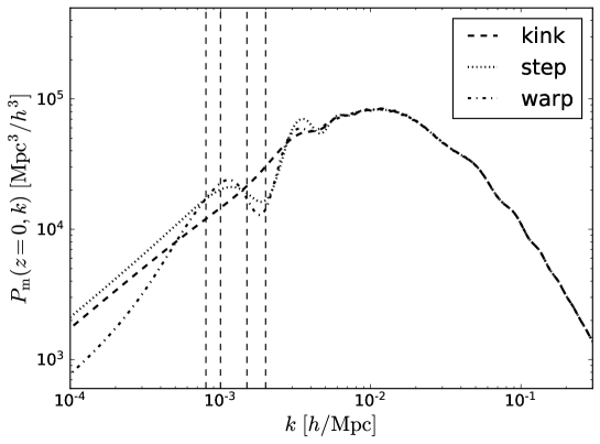
Figure 2: The best fit from Planck 2015 for the matter power spectrum, for the three primordial feature models. Dashed vertical lines correspond to the contour lines in figure 3.

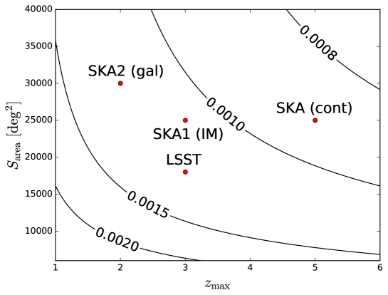
Figure 3: The sky area and maximum redshift of the surveys considered. Contours for $k_{\mathrm{min}}={0.0008},0.001,0.0015,0.002\,h/$Mpc indicate the largest accessible scale estimated to be contained in the survey volume.

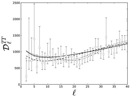
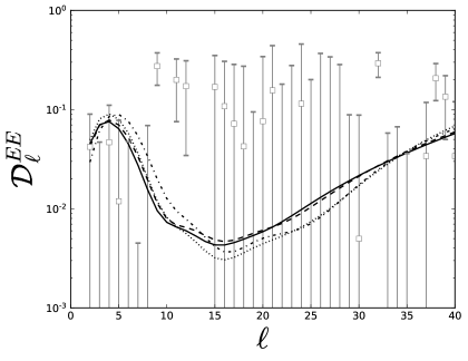
Figure 4: The left (right) panel shows the Planck 2015 temperature (E-mode polarization) data compared to the best fit spectra for $\Lambda$CDM (solid black line) and the three primordial feature models (broken lines – see Fig. 2).

Figure 2 shows the best fit-matter power spectra for the three models, and figure 3 indicates some characteristic scales of the models in the sky area/ maximum redshift plane. The largest-scale contours are calculated from the comoving volume:

$$V_{\rm surv}={4\pi\over 3}f_{\rm sky}\big{[}r(z_{\rm max})^{3}-r(z_{\rm min})^{3}\big{]},\qquad k_{\mathrm{min}}={2\pi\over V_{\rm surv}^{1/3}}\,.$$ (3.1)

Figure 4 compares the $\Lambda$CDM Planck 2015 TT and EE power spectra with those of the primordial feature models.

We write the primordial power spectrum as the standard featureless one $\mathcal{P}_{\mathcal{R},0}$, modulated by the contribution due to the violation of slow-roll:

$$\mathcal{P}_{\mathcal{R}}(k)=\mathcal{P}_{\mathcal{R},0}(k)\cdot\mathcal{P}_{\mathcal{R},1}(k)\,,\qquad\mathcal{P}_{\mathcal{R},0}(k)=A_{\rm s}\left({k\over k_{*}}\right)^{n_{\rm s}-1}\,.$$ (3.2)

3.1 Kink model

This model has a sharp change in the slope of the inflaton potential, which is constant near the transition [71]. After the transition the second slow-roll parameter $\epsilon_{2}$ becomes large for some time because of the discontinuity in the first derivative of the potential – afterwards, slow-roll is recovered. The two different slopes of the potential lead to different asymptotic values of the curvature power spectrum, plus an oscillatory pattern in between. The contribution to $\mathcal{P}_{\mathcal{R}}$ can be derived analytically:

$$\mathcal{P}_{\mathcal{R},1}(y)={} 1+\frac{9}{2}\mathcal{A}_{\mathrm{kink}}^{2}\left(\frac{1}{y}+\frac{1}{y^{3}}\right)^{2}+\frac{3}{2}\mathcal{A}_{\mathrm{kink}}\left(4+3\mathcal{A}_{\mathrm{kink}}-3\frac{\mathcal{A}_{\mathrm{kink}}}{y^{4}}\right)^{2}\frac{1}{y^{2}}\cos(2y)$$

$${}+3\mathcal{A}_{\mathrm{kink}}\left(1-\frac{1+3\mathcal{A}_{\mathrm{kink}}}{y^{2}}-\frac{3\mathcal{A}_{\mathrm{kink}}}{y^{4}}\right)^{2}\frac{1}{y}\sin(2y)\,,\quad y\equiv{k\over k_{\mathrm{kink}}}\,.$$ (3.3)

Here the scale of the transition is $k_{\mathrm{kink}}$, the amplitude is $\mathcal{A}_{\mathrm{kink}}=(A_{+}-A_{-})/A_{+}$, and we use the approximation $|A_{+}\phi|\,,|A_{-}\phi|\ll V_{0}$.

The best fit for the two extra parameters obtained from Planck TT+lowP is $\mathcal{A}_{\mathrm{kink}}=0.089$, $\log\left(k_{\mathrm{kink}}\,\text{Mpc}\right)=-3.05$. This provides an improvement in the fit of CMB data of $\Delta\chi^{2}\simeq-4.5$ [19].

3.2 Step model

A step-like feature in the inflaton potential with a discontinuity of the second derivative of the potential leads to a localized oscillatory pattern with a negligible difference in the asymptotic amplitudes of $\mathcal{P}_{\mathcal{R}}$. There is an analytical approximation, up to second order in the Green’s function expansion [74, 72, 20]:

$$\mathcal{P}_{\mathcal{R},1}(y) = \exp\Big{\{}\mathcal{I}_{0}(y)+\ln\Big{[}1+\mathcal{I}_{1}^{2}(y)\Big{]}\Big{\}}\,,\qquad y\equiv{k\over k_{\mathrm{step}}}\,,$$ (3.4)

where $k_{\mathrm{step}}$ is the inverse of the oscillation frequency. The first- and second-order parts are

$$\mathcal{I}_{0}(y) = \Big{[}C_{1}W(y)+C_{2}W^{\prime}(y)+C_{3}Y(y)\Big{]}\mathcal{D}\left(\frac{y}{x_{\rm step}}\right)\,,$$ (3.5)

$$\sqrt{2}\,\mathcal{I}_{1}(y) = \frac{\pi}{2}\left(1-n_{\rm s}\right)+\Big{[}C_{1}X(y)+C_{2}X^{\prime}(y)+C_{3}Z(y)\Big{]}\mathcal{D}\left(\frac{y}{x_{\rm step}}\right)\,,$$ (3.6)

where $x_{\mathrm{step}}$ is the damping scale, a prime denotes ${\rm d}/{\rm d}\ln y$, and the damping envelope is:

$$\mathcal{D}(y)=\frac{y}{\sinh y}\,.$$ (3.7)

The window functions are:

$$W(y) =\frac{3\sin(2y)}{2y^{3}}-\frac{3\cos(2y)}{y^{2}}-\frac{3\sin(2y)}{2y}\,,$$ (3.8)

$$X(y) =\frac{3}{y^{3}}\left(\sin y-y\cos y\right)^{2}\,,$$ (3.9)

$$Y(y) =\frac{6y\cos(2y)+(4y^{2}-3)\sin(2y)}{y^{3}}\,,$$ (3.10)

$$Z(y) =-\frac{3+2y^{2}-(3-4y^{2})\cos(2y)-6y\sin(2y)}{y^{3}}\,.$$ (3.11)

The step model has 3 parameters:

$$C_{1}=C_{3}=0\,,~{}~{}C_{2}=\mathcal{A}_{\rm step}\,,~{}~{}k_{\rm step}\,,~{}~{}x_{\rm step}\,,$$ (3.12)

and its $\Delta\chi^{2}$ is $\simeq-8.6$ for Planck TT+lowP, corresponding to the best fit parameters $\mathcal{A}_{\rm step}=0.374$, $\log\left(k_{\rm step}\,\text{Mpc}\right)=-3.1$, and $\ln x_{\rm step}=0.342$ [19].

3.3 Warp model

In DBI models, a step in the potential affects also the kinetic term of the Lagrangian, leading to additional signatures in $\mathcal{P}_{\mathcal{R}}$ – this is the warp model [73]. This extention of the step model has 5 parameters: all three $C_{a}$ in (3.5)–(3.6) are nonzero. For the warp model, the $\Delta\chi^{2}$ increases to $-12.1$ for Planck TT+lowP, given the cost of adding five extra parameters [19]. The best fit to Planck TT+lowP is $C_{1}=-1.05$, $C_{2}=\mathcal{A}_{\rm warp}=1.16$, $C_{3}=-0.737$, $\log\left(k_{\rm step}\ \text{Mpc}\right)=-3.12$, and $\ln x_{\rm step}=-0.195$.

4 Results

We forecast the constraints on the $\mathcal{P}_{\mathcal{R}}$ parameters above, for the LSST and SKA surveys (with and without Planck data), in order to quantify the possibility of discriminating these models from a standard power law. (In the limit of a zero amplitude, we recover standard power law predictions for all 3 models.) In the appendix, we give the constraints on the standard cosmological parameters with and without the inclusion of the CMB and show the contours together with the constraints on the primordial-feature parameters from the CMB alone as comparison.

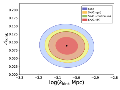
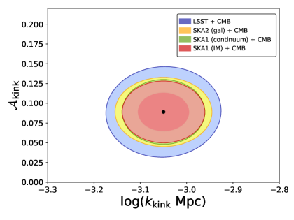
Figure 5: Marginalized 68% and 95% CL contours for the kink model parameters, $k_{\mathrm{kink}}$ and $\mathcal{A}_{\mathrm{kink}}$, using the surveys alone (left), and combining survey and CMB Fisher information (right).

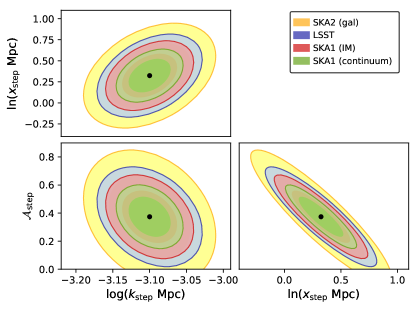
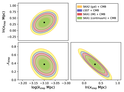
Figure 6: As in figure 5, for the parameters of the step model.

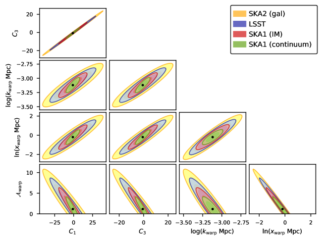
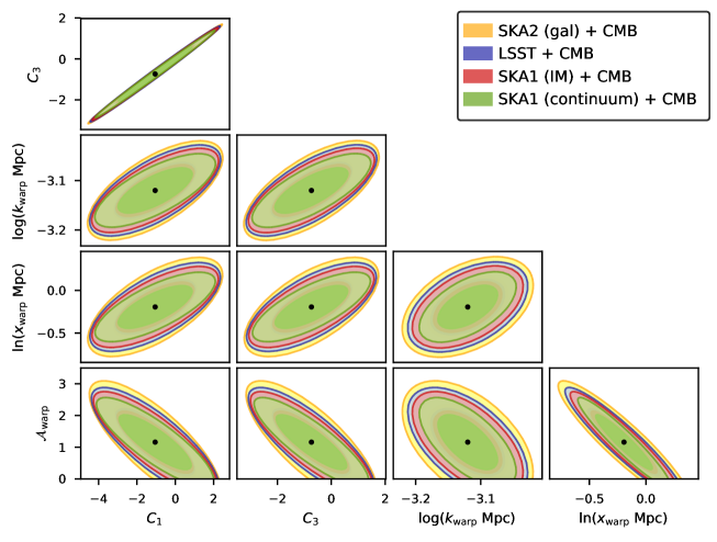
Figure 7: As in figures 5 and 6, for the parameters of the warp model.

We use 5 redshift bins for all the surveys. We have checked that increasing the number of bins to $\sim 10$ or even $\sim 20$ does not change the constraints by more than $1\sigma$, in particular when CMB is added. For LSST and SKA1 IM, we consider the same 5 redshift bins since they cover the same redshift range – with redshift edges 0.15, 0.5, 1, 1.5, 2.2, 3. These bins have approximately the same comoving radial extent. For the SKA2 HI galaxy redshift survey, we use different edges because of the different redshift range considered for this survey. For the SKA1 continuum survey we assume 5 bins with edges 0, 0.5, 1, 1.5, 2, 5.

Measurement of the power spectrum is affected by the $k$-space window function which depends on the limited survey volume observed. We used a top-hat window function. We checked that with a Gaussian window function as in [34, 35], the constraints are changed by less than 5%, thanks to the huge volume covered by these surveys.

Figure 5 shows the forecast constraints for the kink model. For this model there are already strong constraints from Planck 2015 data [19], mainly thanks to the oscillatory pattern which leaves an imprint on intermediate scales. The best fit from CMB data suggests small deviations from the standard power law prediction, which correspond to 20% at $k\simeq 0.001\,h$/Mpc and less than 10% at $k\simeq 0.01\,h$/Mpc. The results obtained in [37], using spectroscopic surveys with smaller volume than LSST and SKA, showed a significant improvement in the constraints on the extra parameters with respect to CMB data, thanks to the possibility of recovering the oscillatory pattern in the 3D matter power spectrum. In [37] it was found that the amplitude could be constrained at more than $1\sigma$. By using larger-volume surveys, Fig. 5 shows that this model can be distinguished from the simplest power-law spectrum at more than $3\sigma$, even without CMB data.

We show in figure 6 the forecast constraints for the parameters of the step model. This model with a localized feature leads to bigger deviations from standard slow-roll predictions, up to 40% in the range $0.002\,h/{\rm Mpc}<k<0.006\,h/{\rm Mpc}$. Previous studies [37, 35] found that the combination of optical galaxy surveys (such as Euclid and LSST) and CMB data will not significantly improve constraints, because the feature is located at scales where the galaxy signal to noise is not optimal. Thanks to the SKA it will be possible to test the current Planck 2015 best fit for this model at more than $3\sigma$, as shown by figure 6. We find that the $1\sigma$ constraint on the amplitude goes from 0.2 for LSST to 0.009 for the SKA1 radio continuum survey.

Figure 7 shows the forecast constraints for the parameters of the warp model. The CMB best fit for this model shows more pronounced features around $k\sim 0.002\,h/$Mpc. The relative difference with respect to the slow-roll predictions of the $\Lambda$CDM model is larger for this model than for the previous two models, but the degeneracy among the five extra parameters makes it difficult to test its predictions with large-scale structure alone. Another important difference is that for this model the oscillations on intermediate scales are smaller, almost absent, and the extent of large-scale suppression in this model, relegated to very large scales $k<0.0005\,h/$Mpc, is not constrained. The degeneracy among the extra parameters of this model is partially broken when the CMB information is added. We find that the combination of large-scale structure and CMB data is really promising, in particular to constrain more complex models such as this one.

4.1 The impact of systematics on the largest scales

One of the most important challenges in observing on ultra-large scales in the matter distribution is the presence of foreground and systematic contamination; see for example different studies on systematic uncertainties in BOSS data [76, 77, 78]. Here we make a rough estimate of the effect of foreground and systematic contamination as follows: we mimic the effect of losing information on the largest scales by increasing $k_{\rm min}$ in (3.1) by a factor of 2, 3, 4, and 5.

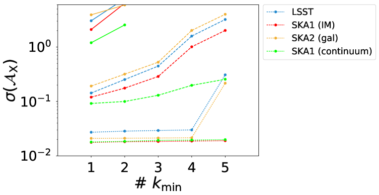
Figure 8: Errors on the amplitude ${\cal A}_{\rm X}$ for $X=$ kink, step, and warp models, from bottom to top respectively, when the theoretical $k_{\rm min}$ is increased by factors of 2,3,4,5. For each model, the errors from the 4 surveys are shown: LSST (blue), SKA1 IM (red), SKA2 galaxy (yellow), and SKA1 continuum (green).

The results in figure 8 show that for the kink model, the constraints on the amplitude of the feature are quite robust when $k_{\rm min}$ is increased. We find a bigger impact on the step model, in particular when $k_{\rm min}$ is more than three times larger than the prediction of (3.1). Finally, for the warp model the amplitude of the feature is unconstrained if we lose the scales $k\lesssim 2k_{\rm min}$.

4.2 The impact of scale-dependent bias

Models with deviations from the standard slow-roll inflation generate specific shapes in the bispectrum (see [79] for a review), so that primordial features can also be searched for in the bispectrum [80], or jointly in the power spectrum and bispectrum [81, 82, 83]. We investigate the additional effect of a scale-dependent bias in the galaxy power spectrum induced by the presence of primordial non-Gaussianity from the primordial features.

We use the analytic expressions for the scale-dependent bias from the integrated perturbation theory formalism [84]:

$$\Delta b(k) \simeq \frac{\sigma_{\rm M}^{2}}{2\delta_{\textrm{c}}}\left[A_{2}\,\mathcal{I}(k)+A_{1}\frac{\partial\mathcal{I}(k)}{\partial\ln\sigma_{\textrm{M}}}\right]\,,$$ (4.1)

$$\mathcal{I}(k) \simeq \frac{1}{\sigma_{\mathrm{M}}^{2}P(k)}\int\frac{d^{3}k^{\prime}}{(2\pi)^{3}}W^{2}(k^{\prime}R)B_{\textrm{L}}(k,k^{\prime},|\mathbf{k}-\mathbf{k^{\prime}}|),$$ (4.2)

where $A_{1}$ and $A_{2}$ have been choosen according to [84]. The matter bispectrum is given by

$$B_{\mathrm{L}}(k_{1},k_{2},k_{3})=\mathcal{M}(k_{1})\mathcal{M}(k_{2})\mathcal{M}(k_{3})B_{\Phi}(k_{1},k_{2},k_{3}),~{}~{}\delta_{\mathrm{m}}(k)=\mathcal{M}(k)\Phi(k)\,.$$ (4.3)

For the step model, we considered the analytical template, up to the second order in the Green’s function expansion, derived in [85].

For the three primordial feature models, the equilateral configuration is the dominant one, as shown by [86]. Hence the scale-dependent bias is not enhanced for this class of models as it would be for a local-type primordial non-Gaussianity. By including a scale-dependent bias due to the primordial non-Gaussian signal sourced by only the violation of slow-roll, we find a small improvement on the constraints, around 3%, on both the amplitude and the position of the feature.

5 Conclusions

In this paper we investigated how well some future LSS surveys will be able to improve current CMB constraints on features in the primordial power spectrum. Such features may be related to the large-scale anomalies in the CMB angular power spectra, seen in Planck [19] and previously in WMAP [16] data. We focused on effects on the largest scales; features on intermediate and smaller scales of the primordial power spectrum have been studied by combining CMB with LSS data in [35, 36, 37, 38, 41, 43].

We showed that the upcoming photometric survey with LSST and radio surveys with SKA can significantly improve the constraints on the extra parameters of models with features localized at ultra-large scales of the matter power spectrum, thanks to the huge volumes probed by these surveys. We performed forecasts for three different models with parametrized features in the primordial power spectrum, namely the kink, step and warp models described in section 3, using galaxy clustering as our observable.

LSST and SKA are expected to improve the constraints on feature models, as shown in figures 5–6-7, due to the large area and redshift range covered. In particular, upcoming intensity mapping and radio continuum surveys in Phase 1 of the SKA will put extremely tight constraints on the parameters of the feature models at more than 3$\sigma$, without adding CMB information. Even if these experiments alone can improve the constraints for such models, the synergies with CMB measurements will be crucial to constrain models with many extra parameters, such as the warp model, as shown in figure 7.

For all three models studied, we find that the SKA1 radio continuum survey gives the tightest constraints on the amplitude of the feature, i.e.

$${\cal A}_{\rm kink}=0.089\pm 0.018\,,\quad{\cal A}_{\rm step}=0.374\pm 0.092\,,\quad{\cal A}_{\rm warp}=1.16\pm 1.20\quad\mbox{at 68\% CL.}$$ (5.1)

We have assumed sufficient redshift information to divide the continuum survey into 5 redshift bins. However, the constraints do not degrade noticeably when 2 bins are used. It appears that volume is more important than redshift information.

We considered the impact of a number of factors that could affect the forecasts:

• Number of redshift bins: increasing the number of bins does not change the constraints by more than $1\sigma$.

• Window function: top-hat or Gaussian choice changes the constraints by less than 5%.

• Systematics on the largest scales: by increasing the largest theoretical scale, corresponding to $k_{\rm min}$, we estimated the degradation of constraints due to loss of information. Figure 8 shows that constraints on the amplitude in the kink model are little affected, those on the step model suffer significantly if we lose scales with $k\lesssim 4k_{\rm min}$, and those on the warp model fall away if we lose scales $k\lesssim 2k_{\rm min}$.

• Scale-dependent bias induced by the non-Gaussianity from primordial features: the inclusion of this extra contribution brings a small improvement of a few % on the constraints.

We have used the galaxy (and intensity) power spectrum in Fourier space, which does not include certain effects on correlations, such as lensing magnification and wide-angle correlations. This means that we lose some information that could improve our constraints. Furthermore, there are other relativistic effects from observing on the past lightcone which grow on ultra-large scales [1, 2, 3, 4, 5, 6, 7, 8, 9, 10, 11, 12, 13, 14, 15]. These effects could lead to some degeneracies with primordial features and thus weaken the constraints at some level. In future work, we will address these two issues by using the galaxy (intensity) angular power spectrum $C_{\ell}^{\rm g}(z,z^{\prime})$, including lensing and all other relativistic effects, as well as wide-angle correlations.

To conclude, we have shown that future photometric and radio surveys can be used to improve our knowledge of the primordial Universe and constrain the hint of deviation from the slow-roll inflation paradigm pointed from current CMB data.

Acknowledgments

MB and RM acknowledge support from the South African SKA Project. MB is also supported by the Claude Leon Foundation, and RM is also supported by the UK STFC (Grant ST/N000668/1). MB, FF and LM acknowledge the support from the grant MIUR PRIN 2015 “Cosmology and Fundamental Physics: Illuminating the Dark Universe with Euclid” and from the agreement ASI n.I/023/12/0 “Attività relative alla fase B2/C per la missione Euclid”. FF wishes to thank UWC for warm hospitality.

Appendix A Additional constraints

We report the uncertainties in the cosmological parameters at 68% CL for the kink, step and warp models in tables 1, 2 and 3 respectively.

Table 1: Constraints on the cosmological parameters for the kink model using LSS surveys alone. In parentheses: combining LSS survey and CMB Fisher information.

	LSST	SKA2 gal	SKA1 IM	SKA1 cont
$\omega_{c}$	0.0017 (0.00030)	0.00078 (0.00028)	0.00087 (0.00028)	0.0013 (0.00030)
$\omega_{b}$	0.00038 (0.000090)	0.00019 (0.000081)	0.00021 (0.000082)	0.00028 (0.000088)
$h$	0.0028 (0.0015)	0.0014 (0.00090)	0.0015 (0.0010)	0.0020 (0.0012)
$n_{s}$	0.0096 (0.0020)	0.0047 (0.0019)	0.0052 (0.0018)	0.0070 (0.0019)
$\log\left(10^{10}A_{s}\right)$	0.051 (0.010)	0.0061 (0.0048)	0.0055 (0.0042)	0.037 (0.0098)
${\cal A}_{\rm kink}$	0.027 (0.023)	0.022 (0.018)	0.018 (0.016)	0.018 (0.016)
$\log\left(k_{\rm kink}\,{\rm Mpc}\right)$	0.058 (0.050)	0.050 (0.042)	0.039 (0.036)	0.039 (0.036)

Table 2: As in Table 1, for the step model.

	LSST	SKA2 gal	SKA1 IM	SKA1 cont
$\omega_{c}$	0.0014 (0.00028)	0.00069 (0.00022)	0.00071 (0.00023)	0.00099 (0.00026)
$\omega_{b}$	0.00027 (0.000083)	0.00014 (0.000061)	0.00014 (0.000065)	0.00020 (0.000076)
$h$	0.0051 (0.0030)	0.0028 (0.0022)	0.0029 (0.0020)	0.0037 (0.0023)
$n_{s}$	0.0095 (0.0022)	0.0047 (0.0020)	0.0053 (0.0020)	0.0069 (0.0021)
$\log\left(10^{10}A_{s}\right)$	0.052 (0.0091)	0.0083 (0.0052)	0.0072 (0.0053)	0.038 (0.0089)
${\cal A}_{\rm step}$	0.14 (0.12)	0.19 (0.14)	0.12 (0.11)	0.092 (0.084)
$\log\left(k_{\rm step}\,{\rm Mpc}\right)$	0.029 (0.022)	0.036 (0.025)	0.024 (0.19)	0.018 (0.016)
$\ln\left(x_{\rm step}\,{\rm Mpc}\right)$	0.20 (0.17)	0.25 (0.19)	0.17 (0.15)	0.13 (0.12)

Table 3: As in Table 1, for the warp model.

	LSST	SKA2 gal	SKA1 IM	SKA1 cont
$\omega_{c}$	0.0014 (0.00028)	0.00069 (0.00022)	0.00070 (0.00023)	0.0010 (0.00026)
$\omega_{b}$	0.00028 (0.000082)	0.00014 (0.000061)	0.00014 (0.000065)	0.00020 (0.000076)
$h$	0.0054 (0.0030)	0.0029 (0.0022)	0.0029 (0.0021)	0.0039 (0.0024)
$n_{s}$	0.0095 (0.0022)	0.0047 (0.0020)	0.0053 (0.0020)	0.0069 (0.0021)
$\log\left(10^{10}A_{s}\right)$	0.052 (0.011)	0.0083 (0.0055)	0.0073 (0.0057)	0.037 (0.011)
${\cal A}_{\rm warp}$	3.0 (0.70)	3.9 (0.78)	2.1 (0.64)	1.2 (0.35)
$\log\left(k_{\rm warp}\,{\rm Mpc}\right)$	0.12 (0.037)	0.15 (0.040)	0.088 (0.034)	0.054 (0.027)
$\ln\left(x_{\rm warp}\,{\rm Mpc}\right)$	0.73 (0.21)	0.92 (0.23)	0.52 (0.19)	0.31 (0.13)
$C_{1}$	12.2 (1.34)	16.0 (1.4)	7.5 (1.3)	3.6 (0.45)
$C_{3}$	7.6 (0.94)	9.9 (0.98)	4.8 (0.91)	2.4 (0.29)

Appendix B Comparison with CMB

We show the marginalized 68% and 95%CL for the kink, step and warp models using the CMB alone versus the combination of LSS surveys with CMB in figures 9, 10 and 11 respectively.

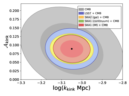
Figure 9: As in figure 5 plus the constraints from CMB alone.

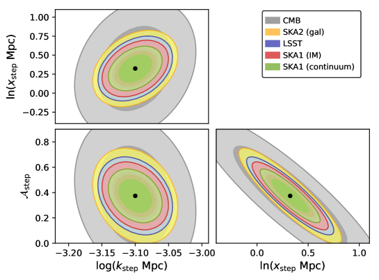
Figure 10: As in figure 6 plus the constraints from CMB alone.

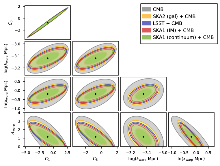
Figure 11: As in figure 7 plus the constraints from CMB alone.

References

- [1] J. Yoo, N. Hamaus, U. Seljak and M. Zaldarriaga, “Going beyond the Kaiser redshift-space distortion formula: a full general relativistic account of the effects and their detectability in galaxy clustering,” Phys. Rev. D 86, 063514 (2012) [arXiv:1206.5809 [astro-ph.CO]].
- [2] S. Camera, M. G. Santos, P. G. Ferreira and L. Ferramacho, “Cosmology on Ultra-Large Scales with HI Intensity Mapping: Limits on Primordial non-Gaussianity,” Phys. Rev. Lett. 111 (2013) 171302 [arXiv:1305.6928 [astro-ph.CO]].
- [3] S. Camera, M. G. Santos and R. Maartens, “Probing primordial non-Gaussianity with SKA galaxy redshift surveys: a fully relativistic analysis,” Mon. Not. Roy. Astron. Soc. 448 (2015) no.2, 1035 [arXiv:1409.8286 [astro-ph.CO]].
- [4] S. Camera, R. Maartens and M. G. Santos, “Einstein’s legacy in galaxy surveys,” Mon. Not. Roy. Astron. Soc. 451 (2015) no.1, L80 [arXiv:1412.4781 [astro-ph.CO]].
- [5] S. Camera et al., “Cosmology on the Largest Scales with the SKA,” PoS AASKA 14 (2015) 025 [arXiv:1501.03851 [astro-ph.CO]].
- [6] A. Raccanelli, F. Montanari, D. Bertacca, O. Doré and R. Durrer, “Cosmological Measurements with General Relativistic Galaxy Correlations,” JCAP 1605, no. 05, 009 (2016) [arXiv:1505.06179 [astro-ph.CO]].
- [7] D. Alonso, P. Bull, P. G. Ferreira, R. Maartens and M. Santos, “Ultra large-scale cosmology in next-generation experiments with single tracers,” Astrophys. J. 814 (2015) no.2, 145 [arXiv:1505.07596 [astro-ph.CO]].
- [8] T. Baker and P. Bull, “Observational signatures of modified gravity on ultra-large scales,” Astrophys. J. 811 (2015) 116 [arXiv:1506.00641 [astro-ph.CO]].
- [9] D. Alonso and P. G. Ferreira, “Constraining ultra large-scale cosmology with multiple tracers in optical and radio surveys,” Phys. Rev. D 92, no. 6, 063525 (2015) [arXiv:1507.03550 [astro-ph.CO]].
- [10] J. Fonseca, S. Camera, M. Santos and R. Maartens, “Hunting down horizon-scale effects with multi-wavelength surveys,” Astrophys. J. 812 (2015) no.2, L22 [arXiv:1507.04605 [astro-ph.CO]].
- [11] A. Raccanelli, M. Shiraishi, N. Bartolo, D. Bertacca, M. Liguori, S. Matarrese, R. P. Norris and D. Parkinson, “Future Constraints on Angle-Dependent Non-Gaussianity from Large Radio Surveys,” Phys. Dark Univ. 15, 35 (2017) [arXiv:1507.05903 [astro-ph.CO]].
- [12] P. Bull, “Extending cosmological tests of General Relativity with the Square Kilometre Array,” Astrophys. J. 817 (2016) no.1, 26 [arXiv:1509.07562 [astro-ph.CO]].
- [13] E. Di Dio, F. Montanari, A. Raccanelli, R. Durrer, M. Kamionkowski and J. Lesgourgues, “Curvature constraints from Large Scale Structure,” JCAP 1606, no. 06, 013 (2016) [arXiv:1603.09073 [astro-ph.CO]].
- [14] D. Alonso, E. Bellini, P. G. Ferreira and M. Zumalacárregui, “Observational future of cosmological scalar-tensor theories,” Phys. Rev. D 95, no. 6, 063502 (2017) [arXiv:1610.09290 [astro-ph.CO]].
- [15] C. S. Lorenz, D. Alonso and P. G. Ferreira, Phys. Rev. D 97 (2018) no.2, 023537 doi:10.1103/PhysRevD.97.023537 [arXiv:1710.02477 [astro-ph.CO]].
- [16] H. V. Peiris et al. [WMAP Collaboration], “First year Wilkinson Microwave Anisotropy Probe (WMAP) observations: Implications for inflation,” Astrophys. J. Suppl. 148 (2003) 213 [astro-ph/0302225].
- [17] L. Covi, J. Hamann, A. Melchiorri, A. Slosar and I. Sorbera, “Inflation and WMAP three year data: Features have a Future!,” Phys. Rev. D 74 (2006) 083509 [astro-ph/0606452].
- [18] P. A. R. Ade et al. [Planck Collaboration], “Planck 2013 results. XXII. Constraints on inflation,” Astron. Astrophys. 571 (2014) A22 [arXiv:1303.5082 [astro-ph.CO]].
- [19] P. A. R. Ade et al. [Planck Collaboration], “Planck 2015 results. XX. Constraints on inflation,” Astron. Astrophys. 594 (2016) A20 [arXiv:1502.02114 [astro-ph.CO]].
- [20] V. Miranda and W. Hu, “Inflationary Steps in the Planck Data,” Phys. Rev. D 89 (2014) 8, 083529 [arXiv:1312.0946 [astro-ph.CO]].
- [21] M. Benetti, “Updating constraints on inflationary features in the primordial power spectrum with the Planck data,” Phys. Rev. D 88 (2013) 087302 [arXiv:1308.6406 [astro-ph.CO]].
- [22] R. Easther and R. Flauger, “Planck Constraints on Monodromy Inflation,” JCAP 1402 (2014) 037 [arXiv:1308.3736 [astro-ph.CO]].
- [23] X. Chen and M. H. Namjoo, Phys. Lett. B 739 (2014) 285 [arXiv:1404.1536 [astro-ph.CO]].
- [24] A. Achucarro, V. Atal, B. Hu, P. Ortiz and J. Torrado, “Inflation with moderately sharp features in the speed of sound: Generalized slow roll and in-in formalism for power spectrum and bispectrum,” Phys. Rev. D 90 (2014) no.2, 023511 [arXiv:1404.7522 [astro-ph.CO]].
- [25] D. K. Hazra, A. Shafieloo, G. F. Smoot and A. A. Starobinsky, “Wiggly Whipped Inflation,” JCAP 1408 (2014) 048 [arXiv:1405.2012 [astro-ph.CO]].
- [26] D. K. Hazra, A. Shafieloo and T. Souradeep, “Primordial power spectrum from Planck,” JCAP 1411 (2014) no.11, 011 [arXiv:1406.4827 [astro-ph.CO]].
- [27] B. Hu and J. Torrado, “Searching for primordial localized features with CMB and LSS spectra,” Phys. Rev. D 91 (2015) no.6, 064039 [arXiv:1410.4804 [astro-ph.CO]].
- [28] A. Gruppuso and A. Sagnotti, Int. J. Mod. Phys. D 24 (2015) no.12, 1544008 doi:10.1142/S0218271815440083 [arXiv:1506.08093 [astro-ph.CO]].
- [29] A. Gruppuso, N. Kitazawa, N. Mandolesi, P. Natoli and A. Sagnotti, “Pre-Inflationary Relics in the CMB?,” Phys. Dark Univ. 11 (2016) 68 [arXiv:1508.00411 [astro-ph.CO]].
- [30] D. K. Hazra, A. Shafieloo, G. F. Smoot and A. A. Starobinsky, “Primordial features and Planck polarization,” JCAP 1609 (2016) no.09, 009 [arXiv:1605.02106 [astro-ph.CO]].
- [31] J. Torrado, B. Hu and A. Achucarro, Phys. Rev. D 96 (2017) no.8, 083515 doi:10.1103/PhysRevD.96.083515 [arXiv:1611.10350 [astro-ph.CO]].
- [32] F. Finelli et al. [CORE Collaboration], “Exploring Cosmic Origins with CORE: Inflation,” arXiv:1612.08270 [astro-ph.CO].
- [33] D. K. Hazra, D. Paoletti, M. Ballardini, F. Finelli, A. Shafieloo, G. F. Smoot and A. A. Starobinsky, JCAP 1802 (2018) no.02, 017 doi:10.1088/1475-7516/2018/02/017 [arXiv:1710.01205 [astro-ph.CO]].
- [34] Z. Huang, L. Verde and F. Vernizzi, “Constraining inflation with future galaxy redshift surveys,” JCAP 1204 (2012) 005 [arXiv:1201.5955 [astro-ph.CO]].
- [35] X. Chen, C. Dvorkin, Z. Huang, M. H. Namjoo and L. Verde, “The Future of Primordial Features with Large-Scale Structure Surveys,” JCAP 1611 (2016) no.11, 014 [arXiv:1605.09365 [astro-ph.CO]].
- [36] X. Chen, P. D. Meerburg and M. Münchmeyer, “The Future of Primordial Features with 21 cm Tomography,” JCAP 1609 (2016) no.09, 023 [arXiv:1605.09364 [astro-ph.CO]].
- [37] M. Ballardini, F. Finelli, C. Fedeli and L. Moscardini, “Probing primordial features with future galaxy surveys,” JCAP 1610 (2016) 041 [arXiv:1606.03747 [astro-ph.CO]].
- [38] Y. Xu, J. Hamann and X. Chen, “Precise measurements of inflationary features with 21 cm observations,” Phys. Rev. D 94 (2016) no.12, 123518 [arXiv:1607.00817 [astro-ph.CO]].
- [39] J. B. Muñoz, E. D. Kovetz, A. Raccanelli, M. Kamionkowski and J. Silk, “Towards a measurement of the spectral runnings,” JCAP 1705 (2017) 032 [arXiv:1611.05883 [astro-ph.CO]].
- [40] A. Pourtsidou, “Synergistic tests of inflation,” arXiv:1612.05138 [astro-ph.CO].
- [41] M. A. Fard and S. Baghram, JCAP 1801 (2018) no.01, 051 doi:10.1088/1475-7516/2018/01/051 [arXiv:1709.05323 [astro-ph.CO]].
- [42] G. A. Palma, D. Sapone and S. Sypsas, arXiv:1710.02570 [astro-ph.CO].
- [43] B. L’Huillier, A. Shafieloo, D. K. Hazra, G. F. Smoot and A. A. Starobinsky, “Probing features in the primordial perturbation spectrum with large-scale structure data,” arXiv:1710.10987 [astro-ph.CO].
- [44] H. Zhan and J. A. Tyson, “Cosmology with the Large Synoptic Survey Telescope,” arXiv:1707.06948 [astro-ph.CO].
- [45] R. Maartens et al. [SKA Cosmology SWG Collaboration], “Overview of Cosmology with the SKA,” PoS AASKA 14 (2015) 016 [arXiv:1501.04076 [astro-ph.CO]].
- [46] F. B. Abdalla et al. [SKA Cosmology SWG Collaboration], “Cosmology from HI galaxy surveys with the SKA,” PoS AASKA 14 (2015) 017 [arXiv:1501.04035 [astro-ph.CO]].
- [47] M. Santos et al. [SKA Cosmology SWG Collaboration], “Cosmology from a SKA HI intensity mapping survey,” PoS AASKA 14 (2015) 019 [arXiv:1501.03989 [astro-ph.CO]].
- [48] M. Jarvis, et al. [SKA Cosmology SWG Collaboration], “Cosmology with SKA Radio Continuum Surveys,” PoS AASKA 14 (2015) 018 [arXiv:1501.03825 [astro-ph.CO]].
- [49] H. J. Seo and D. J. Eisenstein, “Probing dark energy with baryonic acoustic oscillations from future large galaxy redshift surveys,” Astrophys. J. 598 (2003) 720 [astro-ph/0307460].
- [50] Y. S. Song and W. J. Percival, “Reconstructing the history of structure formation using Redshift Distortions,” JCAP 0910 (2009) 004 [arXiv:0807.0810 [astro-ph]].
- [51] Y. Wang, C. H. Chuang and C. M. Hirata, “Toward More Realistic Forecasting of Dark Energy Constraints from Galaxy Redshift Surveys,” Mon. Not. Roy. Astron. Soc. 430 (2013) 2446 [arXiv:1211.0532 [astro-ph.CO]].
- [52] C. Alcock and B. Paczynski, “An evolution free test for non-zero cosmological constant,” Nature 281 (1979) 358.
- [53] N. Kaiser, “Clustering in real space and in redshift space,” Mon. Not. Roy. Astron. Soc. 227 (1987) 1.
- [54] A. J. S. Hamilton, “Linear redshift distortions: A Review,” astro-ph/9708102.
- [55] R. A. Battye, R. D. Davies and J. Weller, “Neutral hydrogen surveys for high redshift galaxy clusters and proto-clusters,” Mon. Not. Roy. Astron. Soc. 355 (2004) 1339 [astro-ph/0401340].
- [56] S. Wyithe and A. Loeb, “Fluctuations in 21cm Emission After Reionization,” Mon. Not. Roy. Astron. Soc. 383 (2008) 606 [arXiv:0708.3392 [astro-ph]].
- [57] T. C. Chang, U. L. Pen, J. B. Peterson and P. McDonald, “Baryon Acoustic Oscillation Intensity Mapping as a Test of Dark Energy,” Phys. Rev. Lett. 100 (2008) 091303 [arXiv:0709.3672 [astro-ph]].
- [58] P. Bull, P. G. Ferreira, P. Patel and M. G. Santos, “Late-time cosmology with 21cm intensity mapping experiments,” Astrophys. J. 803 (2015) no.1, 21W [arXiv:1405.1452 [astro-ph.CO]].
- [59] M. Tegmark, “Measuring cosmological parameters with galaxy surveys,” Phys. Rev. Lett. 79 (1997) 3806 [astro-ph/9706198].
- [60] H. A. Feldman, N. Kaiser and J. A. Peacock, “Power spectrum analysis of three-dimensional redshift surveys,” Astrophys. J. 426 (1994) 23 [astro-ph/9304022].
- [61] L. Knox, “Determination of inflationary observables by cosmic microwave background anisotropy experiments,” Phys. Rev. D 52 (1995) 4307 [astro-ph/9504054].
- [62] G. Jungman, M. Kamionkowski, A. Kosowsky and D. N. Spergel, “Cosmological parameter determination with microwave background maps,” Phys. Rev. D 54 (1996) 1332 [astro-ph/9512139].
- [63] U. Seljak, “Measuring polarization in cosmic microwave background,” Astrophys. J. 482 (1997) 6 [astro-ph/9608131].
- [64] M. Zaldarriaga and U. Seljak, “An all sky analysis of polarization in the microwave background,” Phys. Rev. D 55 (1997) 1830 [astro-ph/9609170].
- [65] M. Kamionkowski, A. Kosowsky and A. Stebbins, “Statistics of cosmic microwave background polarization,” Phys. Rev. D 55 (1997) 7368 [astro-ph/9611125].
- [66] P. A. Abell et al. [LSST Science and LSST Project Collaborations], “LSST Science Book, Version 2.0,” arXiv:0912.0201 [astro-ph.IM].
- [67] Z. M. Ma, W. Hu and D. Huterer, “Effect of photometric redshift uncertainties on weak lensing tomography,” Astrophys. J. 636 (2005) 21 [astro-ph/0506614].
- [68] M. G. Santos et al. [MeerKLASS Collaboration], “MeerKLASS: MeerKAT Large Area Synoptic Survey,” arXiv:1709.06099 [astro-ph.CO].
- [69] S. Yahya, P. Bull, M. G. Santos, M. Silva, R. Maartens, P. Okouma and B. Bassett, “Cosmological performance of SKA HI galaxy surveys,” Mon. Not. Roy. Astron. Soc. 450 (2015) no.3, 2251 [arXiv:1412.4700 [astro-ph.CO]].
- [70] M. Santos, D. Alonso, P. Bull, M. B. Silva and S. Yahya, “HI galaxy simulations for the SKA: number counts and bias,” PoS AASKA 14 (2015) 021 [arXiv:1501.03990 [astro-ph.CO]].
- [71] A. A. Starobinsky, “Spectrum of adiabatic perturbations in the universe when there are singularities in the inflation potential,” JETP Lett. 55 (1992) 489 [Pisma Zh. Eksp. Teor. Fiz. 55 (1992) 477].
- [72] C. Dvorkin and W. Hu, “Generalized Slow Roll for Large Power Spectrum Features,” Phys. Rev. D 81 (2010) 023518 [arXiv:0910.2237 [astro-ph.CO]].
- [73] V. Miranda, W. Hu and P. Adshead, “Warp Features in DBI Inflation,” Phys. Rev. D 86 (2012) 063529 [arXiv:1207.2186 [astro-ph.CO]].
- [74] J. A. Adams, B. Cresswell and R. Easther, “Inflationary perturbations from a potential with a step,” Phys. Rev. D 64 (2001) 123514 [astro-ph/0102236].
- [75] J. Martin, L. Sriramkumar and D. K. Hazra, “Sharp inflaton potentials and bi-spectra: Effects of smoothening the discontinuity,” JCAP 1409 (2014) no.09, 039 [arXiv:1404.6093 [astro-ph.CO]].
- [76] A. J. Ross et al., Mon. Not. Roy. Astron. Soc. 417 (2011) 1350 doi:10.1111/j.1365-2966.2011.19351.x [arXiv:1105.2320 [astro-ph.CO]].
- [77] S. Ho et al., Astrophys. J. 761 (2012) 14 doi:10.1088/0004-637X/761/1/14 [arXiv:1201.2137 [astro-ph.CO]].
- [78] C. Hernández-Monteagudo et al., Mon. Not. Roy. Astron. Soc. 438 (2014) no.2, 1724 doi:10.1093/mnras/stt2312 [arXiv:1303.4302 [astro-ph.CO]].
- [79] X. Chen, “Primordial Non-Gaussianities from Inflation Models,” Adv. Astron. 2010 (2010) 638979 [arXiv:1002.1416 [astro-ph.CO]].
- [80] P. A. R. Ade et al. [Planck Collaboration], “Planck 2015 results. XVII. Constraints on primordial non-Gaussianity,” Astron. Astrophys. 594 (2016) A17 [arXiv:1502.01592 [astro-ph.CO]].
- [81] J. R. Fergusson, H. F. Gruetjen, E. P. S. Shellard and M. Liguori, “Combining power spectrum and bispectrum measurements to detect oscillatory features,” Phys. Rev. D 91 (2015) no.2, 023502 [arXiv:1410.5114 [astro-ph.CO]].
- [82] J. R. Fergusson, H. F. Gruetjen, E. P. S. Shellard and B. Wallisch, “Polyspectra searches for sharp oscillatory features in cosmic microwave sky data,” Phys. Rev. D 91 (2015) no.12, 123506 [arXiv:1412.6152 [astro-ph.CO]].
- [83] P. D. Meerburg, M. Münchmeyer and B. Wandelt, “Joint resonant CMB power spectrum and bispectrum estimation,” Phys. Rev. D 93 (2016) no.4, 043536 [arXiv:1510.01756 [astro-ph.CO]].
- [84] T. Matsubara, “Deriving an Accurate Formula of Scale-dependent Bias with Primordial Non-Gaussianity: An Application of the Integrated Perturbation Theory,” Phys. Rev. D 86 (2012) 063518 [arXiv:1206.0562 [astro-ph.CO]].
- [85] P. Adshead, C. Dvorkin, W. Hu and E. A. Lim, “Non-Gaussianity from Step Features in the Inflationary Potential,” Phys. Rev. D 85 (2012) 023531 [arXiv:1110.3050 [astro-ph.CO]].
- [86] J. O. Gong and M. Yamaguchi, “Correlated primordial spectra in effective theory of inflation,” Phys. Rev. D 95 (2017) no.8, 083510 [arXiv:1701.05875 [astro-ph.CO]].