ADINE: An Adaptive Momentum Method for Stochastic Gradient Descent

Abstract

Two major momentum-based techniques that have achieved tremendous success in optimization are Polyak’s heavy ball method and Nesterov’s accelerated gradient. A crucial step in all momentum-based methods is the choice of the momentum parameter $m$ which is always suggested to be set to less than $1$. Although the choice of $m<1$ is justified only under very strong theoretical assumptions, it works well in practice even when the assumptions do not necessarily hold. In this paper, we propose a new momentum based method ADINE, which relaxes the constraint of $m<1$ and allows the learning algorithm to use adaptive higher momentum (also called ‘inertia’, hence the name ADINE). We motivate our hypothesis on $m$ by experimentally verifying that a higher momentum ($\geq 1$) can help escape saddles much faster. Using this motivation, we propose our method ADINE that helps weigh the previous updates more (by setting the momentum parameter $>1$), evaluate our proposed algorithm on deep neural networks and show that ADINE helps the learning algorithm to converge much faster without compromising on the generalization error.

1 Introduction

Non-convex optimization problems are natural formulations in many machine learning problems (e.g. (Un)supervised learning, Bayesian learning). Various learning approaches have been proposed in such settings, as global minimization of such problems are NP-hard in general. Gradient descent is the de-facto iterative learning algorithm used for such optimization problems in machine learning, especially in deep learning. Several variants of gradient descent methods have been proposed and all thse proposed methods can be broadly classified into momentum-based methods (e.g. Nesterov’s Accelerated Gradient [9]), variance reduction methods (e.g. Stochastic Variance Reduced Gradient [6],[11]) and adaptive learning methods (e.g. AdaGrad [2]).

Gradient descent coupled with momentum - also called classical momentum by Polyak [10], is the first ever variant of gradient descent involving the usage of a momentum parameter. The momentum methods use the information from previous gradients in addition to the current gradient for updating the learning parameters. Nesterov in his seminal work [9], proposed an accelerated gradient method (also a momentum based method as shown by [15]) which gives an upper bound on the number of iterations for learning algorithm to converge. With the tremendous success of deep learning models, Sutskever et al in their work [15] worked out to incorporate the algorithm by Nesterov [9]. Nesterov’s method performs an update in the same way as classical momentum, only with a correction to the gradient.

Gradient descent is generally used in the form of mini-batch gradient descent in minimizing all real world optimization problems, where only a small subset of training data (called a mini-batch) is used due to the presence of enormous amounts of training data. The use of a mini-batch for gradient calculation introduces a lot of variance due to the stochasticity of learning algorithm. Methods like SVRG [6], [11] have been proposed, which try to reduce the variance in gradient with strong theoretical guarantees. There exist other variance reduction methods like SAG [13] and SDCA [14] also.

Recently, several methods have been proposed that try to adapt the learning rate in gradient descent. Riedmiller and Braun proposed Rprop [12] method which suggested the usage of an adaptive learning rate based on the sign of gradient in last two iterates. Rprop increases the learning rate of a weight if the gradient sign does not change in last two iterates, otherwise it decreases the learning rate. AdaGrad - proposed by Duchi et al [2], divides $\eta$(a global learning rate) of every step by the square of the $\ell_{2}$ norm of all previous gradients. This scaling using the norm reduces the learning in dimensions which have already changed significantly, and speeds up in the dimensions that have not changed rapidly, thereby stabilizing the model. RMSProp proposed by Tieleman et al [16] is a simple amalgamation of Rprop and SGD. This method scales the learning rate by the decaying average of squared gradient. There are few other methods proposed which adapts the learning rate like AdaDelta [18]. Adam - proposed by Kingma and Ba [7] is a very successful method that almost all recent state-of-the-art deep learning models used. Adam makes use of the first and second order moments of gradients and ideas from norm-based methods, through combining the advantages from AdaGrad and RMSProp.

In this work, we study momentum-based methods and propose the idea of having scheduled increased momentum. We motivate our work by showing that higher momentum can help escape saddles. We then propose ADINE - an adaptive momentum based method which helps learning algorithms converge faster. The paper is organized as follows: Section 2 discusses existing methods and background, Section 3 discusses the motivation of our work and shows how higher momentums help escape saddles, Section 4 showcases our proposed algorithm ADINE and Section 5 contain experimental results that validate our hypothesis.

2 Background and Previous Work

Let us consider the minimization of a function $f$ w.r.t. parameters denoted by $\mathbf{\theta}$. If this function is convex in nature, the minimization is "easy". But in most real-world problems, such as in deep learning, this function is non-convex in nature, making it "difficult". The gradient descent (abbrev. GD) algorithm has become the workhorse to minimize such non-convex functions. In 1964, Polyak [10] proposed a way to use the previous updates in GD, and this is referred to as Polyak’s heavy ball method or Classical Momentum (abbrev. CM). The update equations of CM are:

$$\mathbf{v}_{t+1}=m\mathbf{v}_{t}-\eta\nabla f\left(\mathbf{\theta}_{t}\right)\hskip 14.22636pt\text{with}\hskip 2.84526pt\mathbf{v}_{0}=\mathbf{0}$$ (1)

$$\mathbf{\theta}_{t+1}=\theta_{t}+\mathbf{v}_{t+1}$$ (2)

Here, $m$ is the momentum parameter, and $\eta$ is the learning rate. However, this method is proven to be theoretically beneficial under very strong conditions (strong convexity and strong smoothness). In 1983, Nesterov’s Accelerated Gradient (abbrev. NAG) [9] given by Nesterov, achieved convergence at the rate of $O\left(\nicefrac{{1}}{{k^{2}}}\right)$ under minimal assumptions (Lipschitz continuity). The update equations of NAG are given below, where $m_{t}$ and $\eta$ stand for momentum and learning rate respectively.

$$\mathbf{y}_{t+1}=\mathbf{\theta}_{t+1}+m_{t}\left(\mathbf{\theta}_{t}-\mathbf{\theta}_{t-1}\right)\hskip 14.22636pt\text{with}\hskip 2.84526pt\mathbf{\theta}_{0}=\mathbf{\theta}_{-1}$$ (3)

$$\mathbf{\theta}_{t+1}=\mathbf{y}_{t+1}-\eta\nabla f\left(\mathbf{y}_{t+1}\right)$$ (4)

$$m_{t}=\frac{a_{t}-1}{a_{t+1}}$$ (5)

$$a_{t}=\frac{1+\sqrt{4a_{t-1}^{2}+1}}{2}\text{ and }a_{0}=1$$ (6)

In our work, we consider the analogous update equations presented by Sutskever et al [15] which characterize NAG. These are as follows:

$$\mathbf{v}_{t+1}=m\mathbf{v}_{t}-\eta\nabla f\left(\mathbf{\theta}_{t}+m\mathbf{v}_{t}\right)\hskip 14.22636pt\text{with}\hskip 2.84526pt\mathbf{v}_{0}=\mathbf{0}$$ (7)

$$\mathbf{\theta}_{t+1}=\mathbf{\theta}_{t}+\mathbf{v}_{t+1}$$ (8)

Theoretical guarantees from CM

Let $f(\cdot)$ be an $\alpha$-strongly convex and $\beta$-smooth function on $\mathbb{R}^{d}$. The heavy ball method achieves an $\epsilon$-accurate solution of $\mathbf{\theta}^{*}$ in

$$O\left(\sqrt{\kappa}\log\left(\frac{1}{\epsilon}\right)\right)$$

steps, where $\kappa:=\frac{\beta}{\alpha}$ is the condition number of the problem and $\eta_{\text{opt}}$ and $m_{opt}$ in equation 1 is given by

$$\eta_{\text{opt}}=\frac{4}{(\sqrt{\beta}+\sqrt{\alpha})^{2}}\quad,\quad m_{\text{opt}}=\left(\frac{\sqrt{\beta}-\sqrt{\alpha}}{\sqrt{\beta}+\sqrt{\alpha}}\right)^{2}$$

Theoretical guarantees from NAG

Let $f(\cdot)$ be a convex function over $\mathbb{R}^{d}$ and $L$-smooth, then NAG achieves an $\epsilon$-accurate solution of $\mathbf{\theta}^{*}$ in

$$O\left(\sqrt{\frac{L}{\epsilon}}\right)$$ (9)

steps, and also ensures that:

$$f(\mathbf{\theta}^{(t)})-f(\mathbf{\theta}^{*})=O\left(\frac{1}{t^{2}}\right)$$ (10)

3 Motivation

A key motivation for our work arises from observing the values of the momentum parameters in CM and NAG. Polyak’s suggested choice of $m<1$ in his method is a general scenario while making use of CM in most optimization problems. We analyze the reason for the choice of $m<1$ in NAG. We refer to the analogue to $a_{t}$ used by Sutskever et al in [15], and its consequence in the approximation of the momentum parameter $m_{t}$, which is:

$$a_{t}=\frac{1+\sqrt{4a_{t-1}^{2}+1}}{2}\approx a_{t-1}+0.5\hskip 14.22636pt\left(\text{For large }a_{t}\right)$$ (11)

$$\implies a_{t}\approx\frac{t+4}{2}\implies m_{t}=\frac{a_{t}-1}{a_{t+1}}\approx\frac{t+2}{t+5}<1$$ (12)

We take CM and analyze the behaviour of the update focusing on the importance of the momentum parameter. We perform a sum over the parameter updates in CM, with $f(\cdot)$ in consideration:

$$\mathbf{\theta}_{t+1}=\mathbf{\theta}_{t}-\eta\nabla f\left(\mathbf{\theta}_{t}\right)+m(\mathbf{\theta}_{t}-\mathbf{\theta}_{t-1})\implies\mathbf{\theta}_{n+1}=m\mathbf{\theta}_{n}+(1-m)\mathbf{\theta}_{0}-\eta\sum_{t=0}^{n}\nabla f\left(\mathbf{\theta}_{t}\right)$$ (13)

Note the effect of $m$ on the previous update, which suggests that higher the momentum parameter, higher the influence of the previous update over the update. Such a correspondence can also be drawn with respect to NAG as well.

The study of momentum in a non-convex setup is interesting because the loss function of a deep neural network (objective function) to be optimized doesn’t satisfy the convexity assumptions Polyak and Nesterov make, and yet has achieved huge success in recent years, prior to the arrival of newer adaptive gradient methods. We believe that the analysis of momentum is still not addressed in its entirety. We start our analysis by investigating to see if we can do any better with existing momentum-based methods by weighing the previous updates more. We hypothesize that setting the momentum parameter higher will help the learning algorithm to converge faster. Another motivation to study the variation of $m$ is the problem of saddles in deep learning models. It has been argued that as the dimensionality of the model increases, existence of local minima is no longer an issue; instead, it is the exponential proliferation of saddle points [1][3] which makes optimization in deep learning slow. We hypothesize that setting momentum to $\geq 1$ can help escape saddles.

4 Proposed Method: ADINE

As mentioned earlier, in most real-world settings for performing gradient descent, especially in deep learning, a variant of gradient descent - mini-batch gradient descent is used. However, the loss computed over a mini-batch is a noisy estimate of the actual loss and depends on the size of the mini-batch taken. To help smoothen this loss relatively, for the use of ADINE, we suggest the use of weighted sum loss, which captures the monotonic nature of the descent as well as the noise that is characteristic of this method. We define this weighted sum loss (abbrev. WSL) as:

$$\hat{l}_{k}=\frac{\hat{l}_{k-1}+l_{k}}{2}\hskip 8.53581pt\text{with}\hskip 8.53581pt\hat{l}_{1}=\frac{l_{1}}{2}\hskip 14.22636pt\leftrightarrow\hskip 14.22636pt\hat{l}_{k}=\displaystyle\sum_{i=1}^{k}\frac{l_{i}}{\left(2^{k-i+1}\right)}$$ (14)

Here $l_{k}=l(\mathbf{\theta}_{k})$ and $\hat{l}_{k}$ stands for the WSL computed after $k$ iterations. Noticeably, the first form is recursive, and the second form is a closed form expression. Using this definition of WSL, we propose our ADaptive INErtia algorithm, ADINE, below.

Algorithm 1 ADINE (ADaptive INErtia), the proposed algorithm

0:  $\mathbf{\theta}_{0}$: Initial parameters

0:  $l(\cdot)$: Loss Function

0:  $\eta$: Learning Rate

0:  $m_{s},m_{g}$: Standard momentum ($<1$) and Greater momentum ($\geq 1$)

0:  $\zeta>0$: ADINE hyperparameter to control tolerance

1:  $t\leftarrow 0$, $\hat{l}_{0}\leftarrow 0$, $\mathbf{v}_{0}\leftarrow\mathbf{0}$ (Initialize timestep, weighted-sum-loss and velocity vector)

2:  $m\leftarrow m_{s}$ (Initialize the momentum parameter)

3:  while until convergence of $\mathbf{\theta}_{t}$ do

4:     $t\leftarrow t+1$

5:     Compute current loss $l_{t-1}=l(\mathbf{\theta}_{t-1})$ and weighted-sum-loss $\hat{l}_{t}=\frac{\hat{l}_{t-1}+l_{t}}{2}$

6:     if $\hat{l}_{t}>\zeta\hat{l}_{t-1}$ then

7:        $m\leftarrow m_{s}$

8:     else

9:        $m\leftarrow m_{g}$

10:     end if

11:     $\displaystyle\mathbf{v}_{t}=m\mathbf{v}_{t-1}-\eta\nabla l(\mathbf{\theta}_{t-1}+m\mathbf{v}_{t-1})$

12:     $\displaystyle\mathbf{\theta}_{t}=\mathbf{\theta}_{t-1}+\mathbf{v}_{t}$

13:  end while

14:  return  $\theta_{*}$ (Resulting Parameters)

$\zeta$ is a new hyperparameter that our algorithm takes as input. The intuition for this hyperparameter is as follows: taking into account the noisy nature of updates arising due to mini-batch gradient descent, if the current WSL i.e., $\hat{l}_{k}$ is greater than the previous WSL i.e., $\hat{l}_{k-1}$ within a limit, decided by the $\zeta$ factor, we set momentum to $m_{g}$. If the current WSL is lower than the previous WSL, we are in terms, since this ensures progress. If the current WSL is higher than allowed amount of increase dictated by $\zeta$, then we set momentum to $m_{s}$. Setting higher $\zeta$ allows for higher upper bound/tolerance from above, which could cause your model to train badly. On the contrary, setting lower $\zeta$ allows for a strict upper bound/tolerance, which could cause momentum to not being set to $m_{g}$ at all.

We performed some ablation studies on this new hyperparameter, and we list our observations:

• For wide and shallow networks, a higher choice of $\zeta$ is preferred for better results.

• For narrow and shallow networks, a lower choice of $\zeta$ is preferred for better results.

• For deep networks, a lower choice of $\zeta$ is preferred for better results.

5 Experiments

5.1 Experiments on Synthetic Functions

We first show results to study the hypothesis that higher momentum parameter can help escape saddles. We use a generalized quadratic function of the form

$$f(\mathbf{x})=\mathbf{x}^{T}\Lambda\mathbf{x}$$ (15)

where $\Lambda$ is a diagonal matrix whose entries are sampled from $\mathcal{U}[0.99,1.01]$ and we toggle the signs of the $\Lambda_{ii}$’s alternatively, to ensure that the the critical point $\mathbf{x}^{*}=\mathbf{0}$ is a saddle point. $n$ is the dimensionality of the domain of the function $f$. The results are shown in Figure 1.

We also make use of a generalized cubic function of the form

$$g(\mathbf{x})=\mathbf{x}^{T}\Theta(\mathbf{x}\odot\mathbf{x})$$ (16)

where $\Theta$ is a diagonal matrix whose entries are sampled from $\mathcal{U}[1,2]$, and $\odot$ represents element-wise product. Note that $\nabla^{2}g(\mathbf{0})=\mathbf{0}_{n\times n}$, where $n$ is the dimensionality of the domain of the function $g$, meaning $\mathbf{x}^{*}$ is a saddle-point. The results are shown in Figure 2. Note that both the generalized quadratic 15 and cubic 16 are unbounded.

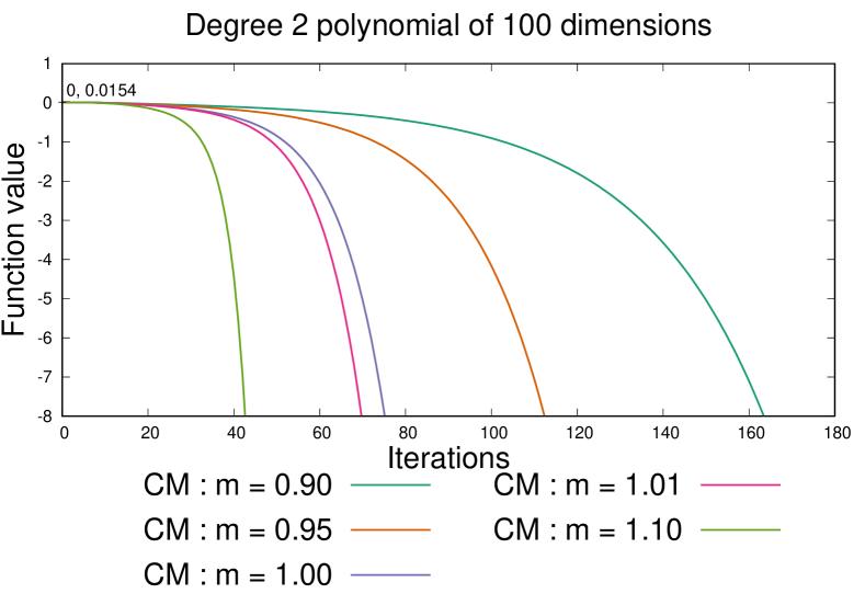
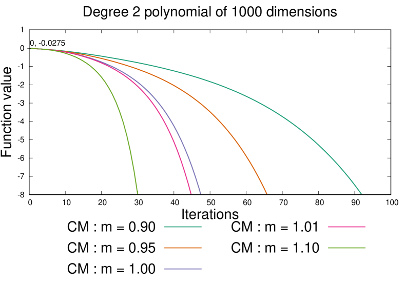
Figure 1: We set $n$ to be 100 and 1000 and used CM until the value of the function was lesser than -8. We use 5 different momentum parameters from the set $\{0.90,0.95,1.00,1.01,1.10\}$. Note how the descent is faster in the case of $m\geq 1$ Very similar kinds of results were observed with NAG. (Best viewed in color)

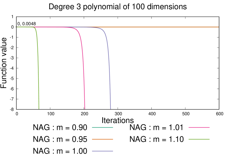
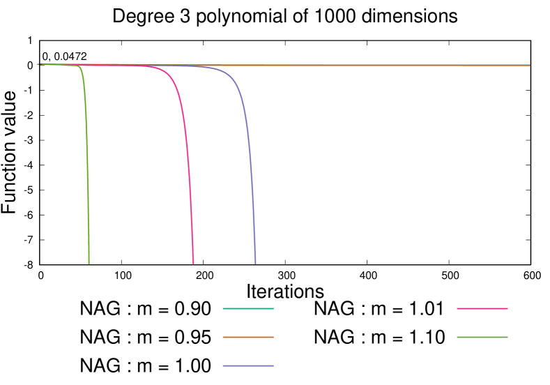
Figure 2: We set $n$ to be 100 and 1000 and used NAG until the value of the function was lesser than -8. We use 5 different momentum parameters from the set $\{0.90,0.95,1.00,1.01,1.10\}$. Note how the descent is faster in the case of $m\geq 1$ Very similar kinds of results were observed with CM. (Best viewed in color)

Perceiving this idea might be harder due to the existence of higher dimensions, which is why we also provide a contour plot of a special case of the function in equation 15 with $n=2$ and $\Lambda=\begin{bmatrix}1&0\\ 0&-1\end{bmatrix}$. We try it with both CM and NAG and wait until the function value dips below -10. The results are tabulated in Table 1 and the traces are shown in Figure 3.

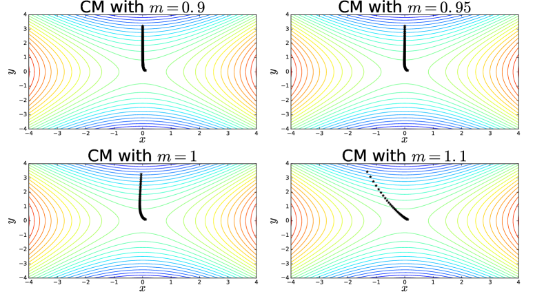
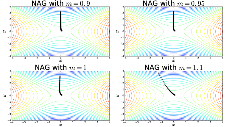
Figure 3: In both subfigures, the top left contour plot is the trace of the updates obtained by setting m to 0.9, the top right contour plot is the trace of the updates obtained by setting m to 0.95, the bottom left contour plot is the trace of the updates obtained by setting m to 1, and the bottom right contour plot is the trace of the updates obtained by setting m to 1.1.

Table 1: Number of iterations taken to reach a function value of -10 with the function $f(x,y)=x^{2}-y^{2}$ using different momentum schemes.

Method	Number of Iterations
CM: m = 0.9	209
CM: m = 0.95	142
CM: m = 1	93
CM: m = 1.1	49

Method	Number of Iterations
NAG: m = 0.9	206
NAG: m = 0.95	140
NAG: m = 1	91
NAG: m = 1.1	49

5.2 Experiments with Neural Networks

We also conducted experiments on deep neural networks, in particular, on classification tasks on CIFAR10 and SVHN and autoencoders trained on MNIST.

5.2.1 Experimental setups for SVHN and CIFAR10 classification tasks

Since our proposed work is an improvement over momentum based methods, we compare our method with the parameterized NAG algorithm due to Sutskever et al[15] with different momentum settings. We use a learning rate of $10^{-4}$ and a weight decay rate of $10^{-4}$. The input to the networks are features extracted from the original images using a pre-trained WideResnet [17], which produces 256 and 192 dimensional vectors for each image CIFAR10 and SVHN respectively.

5.2.2 Experimental setup for MNIST autoencoder task

For MNIST, we use the autoencoder architecture described by Hinton and Salakhutdinov in [5]. We set learning rate and weight decay parameters to be $10^{-4}$ and $10^{-4}$ respectively. We also construct a denser version of the aforementioned architecture with an architecture 784 x 1000 x 500 x 250 x 125 x 60 for the encoder and an architecture 60 x 125 x 250 x 500 x 1000 x 784 for the decoder. Sigmoid activations are placed between hidden layers of the encoder and decoder, but there is no activation between the encoder and the decoder. We use the same parameters as those used to train the earlier autoencoder.

5.2.3 Results

The architectures used for CIFAR10 are 256 x 384 x 256 x 128 x 10 and 256 x 512 x 10 and for SVHN are 192 x 288 x 288 x 10 and 192 x 384 x 10. All these architectures have ReLU[8] activations in the hidden layers and a softmax activation at the output, and are trained with a cross-entropy loss and a batch size of 32. The weights are initialized with the scheme suggested by Glorot and Bengio [4]. ADINE achieves a test accuracy of $\approx 94\%$ on CIFAR10 and $\approx 96\%$ on SVHN. These results are consistent with those obtained with standard momentum methods, but ADINE is able to achieve this accuracy much faster than the standard momentum methods. Variation of the training loss with time has been plotted in the figures 4 and 5.

For the MNIST autoencoder task, the weights have been initialized using the same scheme as earlier, and is trained with a binary cross entropy loss and a batch size of 64. The variation of the training loss with time has been plotted in Figure 6.

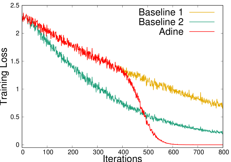
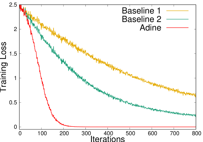
Figure 4: Convergence of training loss of deep neural network on CIFAR-10 architectures 256 x 384 x 256 x 128 x 10 (L) and 256 x 512 x 10 (R). Baseline 1 is NAG with m = 0.9, Baseline 2 is NAG with m = 0.95, ADINE is our proposed method with $m_{s}=0.9$, $m_{g}=1.0001$ and $\zeta=1.03$ (for L) and $\zeta=1.5$ (for R)

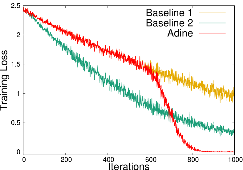
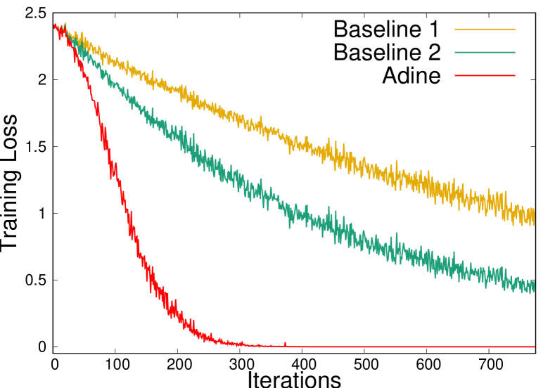
Figure 5: Convergence of training loss of deep neural network on SVHN architectures 192 x 288 x 288 x 10 (L) and 192 x 384 x 10 (R). Baseline 1 is NAG with m = 0.9, Baseline 2 is NAG with m = 0.95, ADINE is our proposed method with $m_{s}=0.9$, $m_{g}=1.0001$ and $\zeta=1.1$ (for L) and $\zeta=1.5$ (for R)

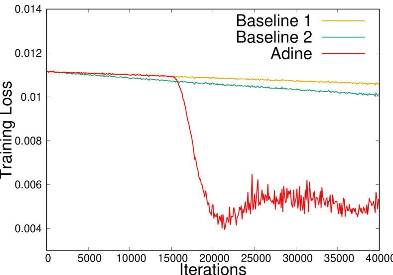
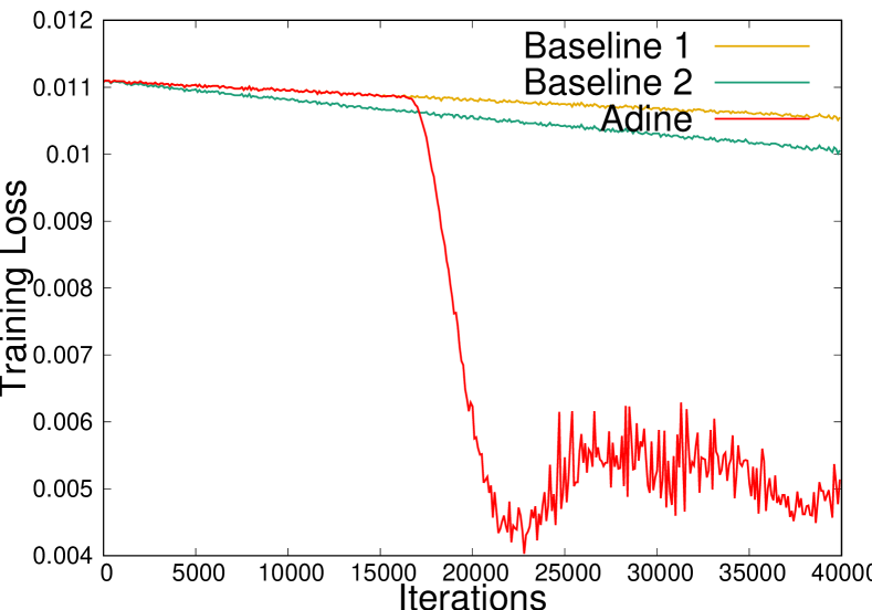
Figure 6: Convergence of training loss of MNIST autoencoder with architecture due to Hinton and Salakhutdinov [5] (L) and encoder-decoder architecture of 784 x 1000 x 500 x 250 x 125 x 60 and 60 x 125 x 250 x 500 x 1000 x 784 respectively (R). Baseline 1 is NAG with m = 0.9, Baseline 2 is NAG with m = 0.95, ADINE is our proposed method with $m_{s}=0.9$, $m_{g}=1.0001$ and $\zeta=1.48$ (for L and R)

6 Conclusion

In this work, we proposed ADINE, a faster and way to train SGD using scheduled momentum, where the momentum parameter is adaptively changed based on a new weighted loss sum value in a given iteration. We showed empirically that when training using the momentum scheme, the proposed method, ADINE, is able to converge much faster. We demonstrated another major implication of our work in trying escape synthetic saddles in polynomial functions. To the best of our knowledge, this is the first work to explore this particular idea of studying SGD with higher momentum parameter values. As future work, we plan to study the theoretical guarantees of our proposed method ADINE.

References

- [1] Yann N Dauphin, Razvan Pascanu, Caglar Gulcehre, Kyunghyun Cho, Surya Ganguli, and Yoshua Bengio. Identifying and attacking the saddle point problem in high-dimensional non-convex optimization. In Advances in neural information processing systems, pages 2933–2941, 2014.
- [2] John Duchi, Elad Hazan, and Yoram Singer. Adaptive subgradient methods for online learning and stochastic optimization. Technical Report UCB/EECS-2010-24, EECS Department, University of California, Berkeley, Mar 2010.
- [3] Rong Ge, Furong Huang, Chi Jin, and Yang Yuan. Escaping from saddle points — online stochastic gradient for tensor decomposition. In Proceedings of The 28th Conference on Learning Theory, volume 40 of Proceedings of Machine Learning Research, pages 797–842. PMLR, 03–06 Jul 2015.
- [4] Xavier Glorot and Yoshua Bengio. Understanding the difficulty of training deep feedforward neural networks. In Proceedings of the Thirteenth International Conference on Artificial Intelligence and Statistics, volume 9 of Proceedings of Machine Learning Research, Chia Laguna Resort, Sardinia, Italy, 2010. PMLR.
- [5] Geoffrey Hinton and Ruslan Salakhutdinov. Reducing the dimensionality of data with neural networks. Science, 313(5786):504 – 507, 2006.
- [6] Rie Johnson and Tong Zhang. Accelerating stochastic gradient descent using predictive variance reduction. In Proceedings of the 26th International Conference on Neural Information Processing Systems - Volume 1, NIPS’13, pages 315–323, USA, 2013. Curran Associates Inc.
- [7] Diederik P. Kingma and Jimmy Ba. Adam: A method for stochastic optimization. In Proceedings of the 3rd International Conference on Learning Representations (ICLR), 2014.
- [8] Vinod Nair and Geoffrey E. Hinton. Rectified linear units improve restricted boltzmann machines. In Proceedings of the 27th International Conference on International Conference on Machine Learning, ICML’10, pages 807–814, USA, 2010. Omnipress.
- [9] Yurii Nesterov. A method of solving a convex programming problem with convergence rate . In Soviet Mathematics Doklady, volume 27, pages 372–376, 1983.
- [10] Boris Teodorovich Polyak. Some methods of speeding up the convergence of iteration methods. USSR Computational Mathematics and Mathematical Physics, 4(5):1–17, 1964.
- [11] Sashank J Reddi, Ahmed Hefny, Suvrit Sra, Barnabas Poczos, and Alex Smola. Stochastic variance reduction for nonconvex optimization. In International conference on machine learning, pages 314–323, 2016.
- [12] M. Riedmiller and H. Braun. A direct adaptive method for faster backpropagation learning: the rprop algorithm. In IEEE International Conference on Neural Networks, pages 586–591 vol.1, 1993.
- [13] Nicolas L Roux, Mark Schmidt, and Francis R Bach. A stochastic gradient method with an exponential convergence _rate for finite training sets. In Advances in Neural Information Processing Systems, pages 2663–2671, 2012.
- [14] Shai Shalev-Shwartz and Tong Zhang. Stochastic dual coordinate ascent methods for regularized loss minimization. Journal of Machine Learning Research, 14(Feb):567–599, 2013.
- [15] Ilya Sutskever, James Martens, George Dahl, and Geoffrey Hinton. On the importance of initialization and momentum in deep learning. In Proceedings of the 30th International Conference on International Conference on Machine Learning - Volume 28, ICML’13, pages III–1139–III–1147. JMLR.org, 2013.
- [16] T. Tieleman and G. Hinton. Lecture 6.5—RmsProp: Divide the gradient by a running average of its recent magnitude. COURSERA: Neural Networks for Machine Learning, 2012.
- [17] Sergey Zagoruyko and Nikos Komodakis. Wide residual networks. In BMVC, 2016.
- [18] Matthew D Zeiler. Adadelta: an adaptive learning rate method. arXiv preprint arXiv:1212.5701, 2012.